Midlatitude cooling caused by geomagnetic field minimum during polarity reversal

Abstract

The climatic effects of cloud formation induced by galactic cosmic rays (CRs) has recently become a topic of much discussion. The CR–cloud connection suggests that variations in geomagnetic field intensity could change climate through modulation of CR flux. This hypothesis, however, is not well-tested using robust geological evidence. Here we present paleoclimate and paleoenvironment records of five interglacial periods that include two geomagnetic polarity reversals. Marine oxygen isotope stages 19 and 31 contain both anomalous cooling intervals during the sea-level highstands and the Matuyama–Brunhes and Lower Jaramillo reversals, respectively. This contrasts strongly with the typical interglacial climate that has the temperature maximum at the sea-level peak. The cooling occurred when the field intensity dropped to <40% of its present value, for which we estimate >40% increase in CR flux. The climate warmed rapidly when field intensity recovered. We suggest that geomagnetic field intensity can influence global climate through the modulation of CR flux.

One of the main goals of paleoclimatology is to reveal factors that control the Earth’s climate. Besides widely accepted climate drivers such as insolation and air–ocean circulation, the effect of clouds induced by galactic cosmic rays (CRs) has recently become a topic of much interest (e.g., 1, 2). Changes in CR flux may affect cloud cover (3, 4) through charge-related processes such as ion-induced nucleation (5) or its effect on the global electric circuit (6), which in turn affect cloud microphysics and formation/radiation of clouds. This would affect the global heat balance by increasing/decreasing albedo (7). Recent observations and modeling support the link between cloud cover and global temperature on decadal time scales (8). A cooling effect caused by the CR-induced clouds was also observed during the Southern Hemisphere Magnetic Anomaly (9), although the interval of observation was too short to be solid confirmation. Longer-term evidence is needed to confirm the CR flux–climate coupling.

An alternative way of testing the CR flux–climate coupling is to examine climate across a huge CR flux change in geological history. The geomagnetic field is a major factor controlling CR flux over longer time scales (10), and geomagnetic reversals are always accompanied by large decreases in field strength, which cause a large increase in CR flux. The Matuyama–Brunhes (MB) and Lower Jaramillo (LJ) geomagnetic polarity reversals provide suitable opportunities for such a test. During these reversals, the field intensity decreased to 10–20% of its present value for several thousand years (11). Additionally, the MB and LJ reversals occurred during interglacial periods, times when the impact of increased cloud cover on climate should be more readily detectable than in glacial periods. In this study, we compare detailed (ca. 200- to 2,000-y resolution) multiproxy climate analyses of five interglacial periods to see whether those with a geomagnetic reversal have unique features, and whether these features can be ascribed to field intensity variation. A pioneering study in this field examined the climatic effects of the extremely low geomagnetic field strength of the Laschamp excursion at ca. 40 ka and did not find an anomalous cool interval induced by a large increase in CR flux (12). The negative result may be due to the short duration of the Laschamp excursion and its occurrence during a glacial interval. The advantages of the present study, targeting the MB and LJ reversals are that i) the duration of extremely weak geomagnetic intensity spans roughly 5,000 y and ii) we search for cooling during warm climates near peak interglacials.

Geological Setting and Core Description.

A 1,700-m-long sediment core from Osaka Bay in southwest Japan (Fig. S1) is ideal for this study. It covers the last 3.1 Ma at a high sedimentation rate (s.r.) (13–17). The core’s age control points between 1,300 ka and 700 ka demonstrate a uniform s.r. (ca. 63 cm/ky) with high linearity (correlation coefficient = 0.999) (14). During interglacial periods, when sea level was above the level of the Kitan Strait sill (Fig. S1), marine conditions predominated in the basin; basin waters were lacustrine when sea level fell below the sill, primarily during glacial periods. After 1.25 Ma [marine oxygen isotope stage (MIS) 37], 21 marine incursions into Osaka Bay have been recognized and alternating marine and freshwater layers are correlated with interglacial–glacial (orbital) cycles (14, 15). Each marine layer records precession-related sea-level variations (14–16). Small half lock-in depths of magnetization, <10 cm estimated for clays in Osaka Bay (17), and the high s.r. make this a good archive of geomagnetic field variation that can resolve submillennial scale features with a phase lag less than 160 y.

Results and Discussion

Diatom, sulfur, and organic carbon isotope analyses reveal six marine layers (Fig. 1). Deposition of each marine layer begins with a postglacial sea-level rise and is terminated by a sea-level drop moving into a glacial period, passing the Osaka Bay sill (15, 18). In MIS 21 the marine layer is separated into two intervals, corresponding to the precession-related cycles (14). The maximum sea-level highstand in each interglacial occurs in the first precession-related sea-level rise. These can be identified as maxima in pelagic diatom proportions, suggesting the easy exchange of open sea water in Osaka Bay (Fig. 1). The diatom-based sea-level peak is supported by other proxies. Near this peak, the proportions of nonarboreal pollen and Alnus spp. (alder, the main component of marsh forest) fall to a minimum, indicating the maximum distance from the core site to the shoreline during the highest sea levels. Sulfur content decreases slightly near the sea-level high, a trend characteristic of a lower terrestrial organic supply when the core site is farthest from the coast or river mouth (Methods). In MISs 19, 21.5, and 31, a peak in organic matter δ¹³C values suggests dominance by marine organic carbon (Methods).

Fig. 1.

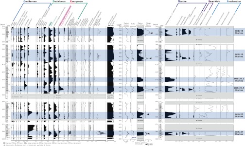
Paleoenvironmental records from Osaka Bay. Left to right: Core lithology, pollen diagram for selected pollen taxa, spore types and other microfossils, organic matter carbon isotope ratios, sulfur content, diatom assemblage compositions, pelagic diatom percentage and diatom diagram for major taxa. Parts of pollen, sulfur, and diatom data are from previous studies (14, 16, 18). The topmost part of the MIS 17 fine clay layer is eroded at 340.34 m.

Marine oxygen isotope data are not directly obtainable for our core owing to the absence of foraminifera fossils (14). However, a linear depth-age model with the average s.r. and calibration of the highest sea level in the core to the minimum of marine oxygen isotope (δ¹⁸O) stack LR04 (19) for each MIS (Table S1) enables us to compare our climate and sea-level proxies with global ice volume changes (Fig. 2). The interglacial (marine) layer is underlain/overlain by layers dominated by subboreal taxa of Picea spp. (spruce) and Abies spp. (fir), indicating the cold and dry climate of glacial periods (Fig. 1). The interglacial vegetation is characterized by deciduous broad-leaved trees such as Fagus spp. (beech) and Quercus subgen. Lepidobalanus spp. (deciduous oak), showing a cool and temperate climate. Among the pollen taxa of interglacials, Fagus and Quercus subgen. Cyclobalanopsis spp. (evergreen oak) are typical elements in the Japanese cool-temperate and warm-temperate zones, respectively, good indicators of cool and warm conditions for interglacial periods.

Fig. 2.

Comparison of climate and sea-level proxies for marine oxygen isotope stages (MISs) 17, 19, 21, 25, and 31. (A) For the warm climate proxy, the proportion of Quercus (Cyclobalanopsis) from an Osaka Bay core is used. (B–D) For the sea-level proxy, the sulfur content and the proportions of marine and pelagic diatoms from the same core are used. No diatom fossils were found at depths 502.23–506.75 m, 571.50–580.20 m, or 585.98–594.65 m (Fig. 1). (E) Marine oxygen isotope stack LR04 (19). Shading indicates thermal maxima based on pollen data. Triangles show the sea-level peak of Osaka Bay. Parts of pollen, sulfur, and diatom data are from previous studies (14, 16, 18). The topmost part of the MIS 17 layer is eroded at 340.34 m.

Comparing the warm proxy to sea-level proxies shows that the thermal maximum occurred in phase with sea-level highstands during MISs 17, 21, and 25, whereas it postdated the sea-level peak in MISs 19 and 31 by several thousand years (Fig. 2). In early MIS 19, Q. (Cyclobalanopsis) percentage gradually increased and Fagus decreased as sea level rose toward the highstand, indicating a progressive warming (Fig. 3 B, C, and G). At about 784 ka, however, the climate trend reversed as Q. (Cyclobalanopsis)/Fagus began to decrease/increase. The high proportion of Fagus from ca. 783–778 ka represents a cool phase. This cool interval is also seen in an objective vegetation reconstruction (Methods and ref. 20), where the temperate deciduous forest (TEDE) biome replaced the broad-leaved evergreen warm-mixed forest (WAMX) (Fig. 3D). The cool phase occurred during the sea-level highstand. It was followed by a rapid warming; the thermal maximum was achieved at ca. 776 ka, well after the highest sea level (Fig. 3).

Fig. 3.

Comparison between geomagnetic field and climate. The graphs cover the time span of the MIS 21 interglacial, the MB polarity transition (Upper), and the entire MIS 31 marine layer (Lower). In the magnetic polarity stratigraphy, black/white shows normal/reverse polarity. (A) Relative paleointensity proxies. The present value is set to 1. Paleomagnetic data for MB are from ref. 18. (B and C) Percentage Fagus and Quercus (Cyclobalanopsis). Pink and blue arrows show the occurrence of warming and cooling, respectively. Red and blue short arrows show a brief warming and cooling, respectively. (D) Reconstructed dominant biome (method in ref. 20). The value obtained by subtracting the affinity score of WAMX (broad-leaved evergreen warm-mixed forest) from that of TEDE (temperate deciduous forest). (E) Mean annual temperature estimated from pollen data using a modern analog method (27), with a red (high) to blue (low) probability gradient. (F) Calculated relative cosmogenic radionuclide (¹⁰Be) production rate from A. (G) Marine oxygen isotope stack LR04 (19). (H) July insolation at 65°N (21).

In MIS 31, Q. (Cyclobalanopsis) increased very slowly through the sea-level highstand at 1,072 ka. The increase accelerated notably at 1,069 ka, reaching its highest proportion at 1,068 ka. The thermal maximum clearly postdated the sea-level highstand with a lag of ∼4,000 y. The proportion of Fagus shows a sharp rise from the base of the marine layer (1,076 ka) and a small decline at the sea-level highstand, which suggests a slight warming at the sea-level maximum. However, the high sea-level interval is clearly dominated by Fagus and the TEDE biome; the relatively cool climate lasted until 1,069 ka. Only after 1,069 ka does the WAMX biome dominate (Fig. 3D).

Cool phases coinciding with sea-level highstands in MIS 19 and 31 are extraordinary because warming and sea-level rise usually occur in phase, as observed in MISs 17, 21, and 25 (Fig. 2), and also in MIS 11 (15). To give one example, in MIS 21 the forest was WAMX, mainly consisting of Quercus (Cyclobalanopsis), and the highest temperature was coincident with the sea-level highstand (Fig. 3). Here we define the cool phase of MISs 19 and 31 as a cooling event that is manifest in vegetation. The onset of the MIS 19 cooling event slightly postdates the northern hemisphere July insolation peak at 787 ka, largely predating the minimum at 776 ka (21) (Fig. 3H), at which the thermal maximum occurred. Thus, the cooling event seems to be unaffected by even direct insolation changes. The MIS 31 cooling event also dovetails with the broad insolation high centered at 1,072 ka. Therefore, the cause of the cooling events is probably independent of orbital forcing, whereas the climate changes in other MISs are controlled by orbital forcing.

The cooling events occurred within polarity transition zones, within intervals of extremely weak magnetic field intensity (Fig. 3). For MIS 19, the cooling event (783–778 ka) lies within the broad weak paleointensity and multiple polarity swing zone (785–776 ka) in the MB transition (18). The multiple polarity swing zone of the MB transition is well documented in multiple locations (18, 22, 23), although deep-sea sediments rarely resolve submillenial features of polarity transition owing to low s.r. (<20 cm/ka), magnetic measurement methodology, and the filtering effects of the postdepositional magnetization process (24). The high-resolution MB transition record from Osaka Bay (s.r. >60 cm/ka) is characterized by very few occurrences of intermediate polarity directions; it is dominated by full normal and reverse polarity fields that change within the range of secular variation (18). Thus, an axial-dipole field component seems to be dominant during the MB transition. These features are confirmed by another high-resolution MB transition record from Java (22) using oriented terrestrial sediment samples. This record includes four successive transitional polarity fields spanning ca. 400 y in duration. Even these seem to be dipolar, because their virtual geomagnetic pole (VGP) positions agree well with the VGP cluster from transitionally magnetized lavas (25). However, it seems unlikely that a tilted dipole would be recorded in this or other records, perhaps because its duration would be too short to be resolved, because few transitional polarity fields have been observed in lavas or high-s.r. sediments.

Unlike the MB transition, the LJ transition lacks multiple polarity swings; although it shows a few intermediate polarity fields, it is similar to the MB transition in that it is dominated by full normal and reverse polarity fields (Fig. S2I). It is thus likely that the geomagnetic field during the LJ transition is also axial-dipolar. A broad paleointensity low spans ca. 1,076–1,067 ka (Fig. S2J), within which the MIS 31 cooling event (1,076–1,069 ka) occurred. Both cooling events occurred during broad paleointensity lows, particularly below about 40% of its present value (Fig. 3). The global paleointensity stack Sint-2000 (1,000-y resolution) also shows a decrease to 10–50% of the present field for the cooling events (11).

Assuming that the fields during polarity transitions are axial-dipolar (18), we convert the relative paleointensity into a cosmogenic radionuclide production rate, a proxy of CR flux controlled by the geomagnetic field (Methods and ref. 26). A CR flux increase of ∼40% is estimated for a paleointensity decrease to 40% of the present level. The cooling event occurred when the high CR flux (>140% of present) was sustained for several thousand years, with a maximum of ∼190% when intensity decreased to 10% (Fig. 3 A and F). Rapid warming occurred synchronously with the recovery of field intensity and CR flux decrease.

The impact on temperature can be estimated from the pollen record using a modern analog technique (Methods and ref. 27). This shows the decrease of mean annual temperature from ∼9 °C to 6 °C when the CR flux was >140% during the MB transition (Fig. 3 E and F). During the LJ reversal temperature decreased from ca. 9 °C to 7 °C at 1,074 ka.

In summary, the temporal agreement between anomalous cool intervals and weak magnetic field intensity suggests that the cooling is primarily caused by the CR flux increase. Magnetic field intensity below ∼40% may be a threshold leading to climate cooling. After 779 ka for the MB and 1,069 ka for the LJ transitions, sharp warming occurred in conjunction with the CR flux decrease associated with the geomagnetic field intensity recovery (Fig. 3).

However, the impact of a 40% reduction may be particular to the MB and LJ reversal and/or the MIS 19 and 31 interglacials. Smaller and/or shorter reductions in field intensity during geomagnetic excursions probably have little effect on climate. For the Laschamp excursion, the North Atlantic and South Atlantic geomagnetic paleointensity stacks from cores of higher-s.r. sediments show a similar sharp decrease in field intensity, much below 40% of the present value (28), and this is consistent with the extremely weak absolute paleointensities estimated from lavas (29, 30). Both stacks indicate a short duration, <1,000 y, which may be the main cause for a weak or unobserved climatic response. The response signal was possibly lost in the low-pass filtered data (cutoff frequency = 1/3,000 y⁻¹) used in the previous study (13). In any case, detection of such short-term climatic response requires high-resolution data that can resolve submillennial scale features. Additionally, the Laschamp excursion occurred during the last glacial period and thus it may be difficult to detect a cooling anomaly.

In contrast, our 100- to 200-y-resolution pollen data reveal submillennial scale climate events. A short-term cooling (∼500 y) at 766–767 ka (Fig. 3 B–E) is correlated with the short-term CR flux increase that corresponds to the extreme paleointensity minimum at 766–767 ka (Fig. 3 A and F). A clear signal of short-term warming is observed around 1,072 ka near the sea-level highstand, within one of the cooling anomalies discussed here. This warming may reflect predominance of orbital forcing at the time of sea-level peak. Finally, a major CR decrease after 775 ka (Fig. 3) has no observable climatic signal, perhaps because the climate was on the way to a glacial. These lines of evidence show that the effect of geomagnetic intensity variations may not always be dominant. It is sometimes negligible due to its short duration, or obscured by the effect of other climate forcings.

A relatively cool climate just before the MB boundary or around substage 19.3 can be seen in the paleoclimate records from central Japan (31), Jordan (32), Italy (33), and Colombia (34) (Fig. 4). The Lake Baikal record is very similar to ours, although the results were not interpreted from a geomagnetic point of view. Biogenic silica contents indicate that the climate was cool at both the MB and LJ polarity transitions, and that the thermal maximum of MISs 19 and 31 clearly postdate the polarity reversals (35). Cooling at reversals may therefore have occurred around the Earth, at least in the low-middle latitudes, but this might not be extended to the polar regions. The deglaciation was not delayed or slowed according to the LR04 data, also evidenced by the fact that the sea-level rise in Osaka Bay did not cease even during the cooling event. No comparable cooling at the MB boundary is seen in the 800-ky deuterium record from the EPICA Dome C ice core (36). The low correlation between CRs and clouds at high latitudes (4, 37) suggests that the CR effect on clouds is less effective near the poles, although more CR flux is expected there than in the low latitudes. A decrease of geomagnetic field does not change the CR flux significantly at high latitude because the CR intensity is limited by atmospheric column density. The climatic effect of CR-induced clouds could be different between low-middle and high latitudes. The use of high-latitude ice core data as a test of the CR effect on climate (12) may not be ideal.

Fig. 4.

Locations of high-resolution climate records for the MB transition (circles) or both the MB and LJ transitions (stars). Cooling events are recorded at low/middle latitudes. 1, Osaka Bay; 2, Boso Peninsula (31); 3, Lake Baikal (35); 4, Jordan Valley (32); 5, Crotone Basin, Italy (33); 6, Bogotá, Colombia (34). Cooling is not seen at 7, Dome C, Antarctica (36).

The anomalous cooling events that coincided with major decreases of field intensity during the MB and LJ polarity reversals suggest that the geomagnetic field can affect the Earth’s climate through modulation of CR flux. Because this mechanistic link is governed by basic geophysical processes that are not specific to any particular geological age, the geomagnetic field may have played an important role in some aspects of long-term climate variation.

Methods

Pollen Analysis.

We extracted fossil pollen from sediment samples by standard physical–chemical methods (14) and identified the extracts under an optical microscope at 400×, with some using the differential interference system. We counted more than 300 (average 407) arboreal pollen (AP) grains for each sediment sample over the entire slide. Nonarboreal pollen (NAP) grains, spores, and fossils of freshwater green algae Pediastrum and marine spore cysts were also identified and counted simultaneously. The individual taxon percentage of arboreal pollen is based on total AP counts. The percentages of NAP, spores, Pediastrum, and cysts were calculated based on the sum of AP, NAP, and spore counts (Fig. 1).

Diatom Analysis.

We treated the samples by standard chemical methods (14) and extracted diatom fossils. At least 300 valves (average 346) were counted for each sample under an optical microscope at 400×, and when necessary, at 1,000× oil immersion or with differential interference equipment or a band-pass filter. Diatom identification and ecological interpretations mainly followed refs. 38 and 39, and the nomenclature in ref. 40. We classified the identified diatoms into three ecological categories, marine, brackish, and freshwater, and calculated their percentages based on total diatoms counted (Fig. 1). Marine zones were defined based on diatom data. We used sulfur data as supplemental evidence if there were no diatoms or numbers were insufficient.

Sulfur Analysis.

Sedimentary sulfur was measured by the turbidimetric method (41). Sulfur content can be a good environmental proxy because it is very sensitive to the content of available organic matter metabolized by sulfate-reducing bacteria (42), and marine (brackish) sediments typically have values greater than 0.3% (43). Note that a reducing environment and/or high organic matter concentration makes the content relatively high (44, 45).

Organic Carbon Isotope Analysis.

Powdered sediments (20–30 mg) were reacted with sulfurous acid (H₂SO₃) in silver foil capsules to remove any carbonate in the sediments, followed by overnight drying in a 50 °C oven. This procedure was repeated as needed. Silver capsules were then wrapped in tin foil. δ¹³C and carbon and nitrogen content were measured on a continuous-flow gas-ratio mass spectrometer (Delta PlusXL; Finnigan). Samples were combusted at 1,000 °C using an elemental analyzer (Costech) coupled to the mass spectrometer. Standardization is based on acetanilide for elemental concentration, NBS-22, and USGS-24 for δ ¹³C. Precision is better than ±0.08 for δ¹³C (1σ), based on repeated internal standards. The δ¹³C values are reported relative to Vienna Pee Dee Belemnite. We only used the data with C/N between 4 and 12 to avoid diagenetically altered samples and samples dominated by terrestrial plant matter. Aquatic organic matter tends to be more negative in lacustrine systems and more positive in brackish/marine waters because of the influence of dissolved inorganic carbon from fluvial or marine sources (46, 47). Carbon isotope ratios in the −27 to −25 range may indicate a freshwater environment and more positive δ¹³C values suggest marine waters. Note, however, that high productivity in a lake can produce algae and plankton with δ¹³C values similar to marine ratios (46).

Paleomagnetic Measurements.

Cubic specimens were cut and put into acrylic boxes of 10 cm³ in volume. We conducted stepwise isothermal remanent magnetization (IRM) acquisition experiments, three-component IRM thermal demagnetization (THD), and measurements of hysteresis parameters on selected specimens. Most of the specimens were subjected to progressive alternating field demagnetizations (AFDs), and some specimens to THDs. Anhysteretic remanent magnetization (ARM) was imparted with a peak AF of 100 mT superimposed on a DC field of 50 μT, and IRM was imparted with a DC field of 2.51 T. For magnetic analyses, we used a 2G cryogenic magnetometer, a MicroMag 3900 vibrating sample magnetometer, and a Bartington MS2 susceptibility meter.

Estimation of CR Flux Modulated by the Geomagnetic Field Intensity.

The relative CR flux is calculated by using the relationship between global average production rate of the most common cosmogenic nuclide, ¹⁰Be, and geomagnetic field intensity for a long-term average solar modulation parameter φ = 550 MeV, as decribed in ref. 26. If we use ¹⁴C or ³⁶Cl as a proxy of the CR flux, the result is broadly similar to the result using ¹⁰Be.

Pollen-Based Quantitative Reconstruction of Vegetation and Climate.

The quantitative vegetation reconstruction uses the biomization method (20). Thirty-two major AP taxa were used for the reconstruction, with percentages recalculated using the sum of the 32 AP taxa.

The quantitative climate reconstruction was done by the modern analog technique (27) with the same 32 AP taxa used for the biomization method. Reconstruction and calibration of its results were performed by Polygon 2.3.3 software (http://dendro.naruto-u.ac.jp/~nakagawa/) using the associated 421 modern pollen and 147 climate datasets. The accuracy of T_ann (mean annual temperature) reconstruction using the datasets was extremely high with R₁ at 0.851 (defined by ref. 27).

References

- 1.Kirkby J. Cosmic rays and climate. Surv Geophys. 2007;28(5):333–375. [Google Scholar]
- 2.Courtillot V, Gallet Y, Le Mouël J-L, Fluteau F, Genevey A. Are there connections between the Earth’s magnetic field and climate? Earth Planet Sci Lett. 2007;253 (3–4):328–339. [Google Scholar]
- 3.Svensmark H, Friis-Christensen E. Variation of cosmic ray flux and global cloud coverage – A missing link in solar-climate relationships. J Atmos Sol Terr Phys. 1997;59(11):1225–1232. [Google Scholar]
- 4.Marsh N, Svensmark H. Solar influence on Earth’s climate. Space Sci Rev. 2003;107(1):317–325. [Google Scholar]
- 5.Kirkby J, et al. Role of sulphuric acid, ammonia and galactic cosmic rays in atmospheric aerosol nucleation. Nature. 2011;476(7361):429–433. doi: 10.1038/nature10343. [DOI] [PubMed] [Google Scholar]
- 6.Tinsley BA. Electric charge modulation of aerosol scavenging in clouds: Rate coefficients with Monte Carlo simulation of diffusion. J Geophys Res. 2010;115:D23211. [Google Scholar]
- 7.Hartmann DL, Ockert-Bell ME, Michelsen ML. The effect of cloud type on Earth’s energy balance: Global analysis. J Clim. 1992;5(11):1281–1304. [Google Scholar]
- 8.Clement AC, Burgman R, Norris JR. Observational and model evidence for positive low-level cloud feedback. Science. 2009;325(5939):460–464. doi: 10.1126/science.1171255. [DOI] [PubMed] [Google Scholar]
- 9.Vieira LEA, da Silva LA. Geomagnetic modulation of cloud effects in the Southern Hemisphere Magnetic Anomaly through lower atmosphere cosmic ray effects. Geophys Res Lett. 2006;33:L14802. [Google Scholar]
- 10.Frank M. Comparison of cosmogenic radionuclide production and geomagnetic field intensity over the last 200,000 years. Philos Trans R Soc Lond A. 2000;358:1089–1107. [Google Scholar]
- 11.Valet J-P, Meynadier L, Guyodo Y. Geomagnetic dipole strength and reversal rate over the past two million years. Nature. 2005;435(7043):802–805. doi: 10.1038/nature03674. [DOI] [PubMed] [Google Scholar]
- 12.Wagner G, Livingstone DM, Masarik J, Muscheler R, Beer J. Some results relevant to the discussion of a possible link between cosmic rays and the Earth’s climate. J Geophys Res. 2001;106 (D4):3381–3387. [Google Scholar]
- 13.Biswas DK, et al. Magnetostratigraphy of Plio-Pleistocene sediments in a 1700-m core from Osaka Bay, southwestern Japan and short geomagnetic events in the middle Matuyama and early Brunhes chrons. Palaeogeograph Palaeoclim Palaeoecol. 1999;148 (4):233–248. [Google Scholar]
- 14.Kitaba I, et al. MIS 21 and the Mid-Pleistocene climate transition: Climate and sea-level variation from a sediment core in Osaka Bay, Japan. Palaeogeograph Palaeoclim Palaeoecol. 2011;299 (1–2):227–239. [Google Scholar]
- 15.Kariya C, Hyodo M, Tanigawa K, Sato H. Sea-level variation during MIS 11 constrained by stepwise Osaka Bay extensions and its relation with climatic evolution. Quat Sci Rev. 2010;29 (15–16):1863–1879. [Google Scholar]
- 16.Kitaba I, Iwabe C, Hyodo M, Katoh S, Matsushita M. High-resolution climate stratigraphy across the Matuyama–Brunhes transition from palynological data of Osaka Bay sediments in southwestern Japan. Palaeogeograph Palaeoclim Palaeoecol. 2009;272 (1–2):115–123. [Google Scholar]
- 17.Hyodo M, Itota C, Yaskawa K. Geomagnetic secular variation reconstructed from wide-diameter cores of Holocene sediments in Japan. J Geomag Geoelectr. 1993;45(8):669–696. [Google Scholar]
- 18.Hyodo M, et al. Millennial- to submillennial-scale features of the Matuyama-Brunhes geomagnetic polarity transition from Osaka Bay, southwestern Japan. J Geophys Res. 2006;111:B02103. [Google Scholar]
- 19.Lisiecki LE, Raymo ME. A Pliocene-Pleistocene stack of 57 globally distributed benthic δ18O records. Paleoceanography. 2005;20:PA1003. [Google Scholar]
- 20.Gotanda K, et al. Biome classification from Japanese pollen data: application to modern-day and Late Quaternary samples. Quat Sci Rev. 2002;21 (4–6):647–657. [Google Scholar]
- 21.Berger A, Loutre MF. Insolation values for the climate of the last 10 million years. Quat Sci Rev. 1991;10(4):297–317. [Google Scholar]
- 22.Hyodo M, et al. High-resolution record of the Matuyama-Brunhes transition constrains the age of Javanese Homo erectus in the Sangiran dome, Indonesia. Proc Natl Acad Sci USA. 2011;108(49):19563–19568. doi: 10.1073/pnas.1113106108. [DOI] [PMC free article] [PubMed] [Google Scholar]
- 23.Channell JET, Hodell DA, Singer BS, Xuan C. Reconciling astrochronological and 40Ar/39Ar ages for the Matuyama-Brunhes boundary and late Matuyama Chron. Geochem Geophys Geosys. 2010;11:Q0AA12. [Google Scholar]
- 24.Hyodo M. Possibility of reconstruction of the past geomagnetic field from homogeneous sediments. J Geomag Geoelectr. 1984;36:45–62. [Google Scholar]
- 25.Singer BS, et al. Structural and temporal requirements for geomagnetic field reversal deduced from lava flows. Nature. 2005;434(7033):633–636. doi: 10.1038/nature03431. [DOI] [PubMed] [Google Scholar]
- 26.Wagner G, et al. Reconstruction of the geomagnetic field between 20 and 60 kyr BP from cosmogenic radionuclides in the GRIP ice core. Nucl Instr Meth Phys Res. 2000;172:597–604. [Google Scholar]
- 27.Nakagawa T, Tarasov PE, Nishida K, Gotanda K, Yasuda Y. Quantitative pollen-based climate reconstruction in central Japan: Application to surface and Late Quaternary spectra. Quat Sci Rev. 2002;21 (18–19):2099–2113. [Google Scholar]
- 28.Stoner JS, Laj C, Channell JET, Kissel C. South Atlantic and North Atlantic geomagnetic paleointensity stacks (0-80 ka): Implications for inter-hemispheric correlation. Quat Sci Rev. 2002;21(10):1141–1151. [Google Scholar]
- 29.Chauvin A, Duncan RA, Bonhommet N, Levi S. Paleointensity of the earth’s magnetic field and K-Ar dating of the Louchadiere volcanic flow (Central France): New evidence for the Laschamp excursion. Geophys Res Lett. 1989;16(10):1189–1192. [Google Scholar]
- 30.Ferk A, Leonhardt R. The Laschamp geomagnetic field excursion recorded in Icelandic lavas. Phys Earth Planet Inter. 2009;177 (1–2):19–30. [Google Scholar]
- 31.Okuda M, et al. MIS11-19 pollen stratigraphy from the 250-m Choshi core, northeast Boso Peninsula, central Japan: Implication for the early/mid-Brunhes (400-780 ka) climate signals. Isl Arc. 2006;15(3):338–354. [Google Scholar]
- 32.Spiro B, et al. Climate variability in the Upper Jordan Valley around 0.78 Ma, inferences from time-series stable isotopes of Viviparidae, supported by mollusk and plant palaeoecology. Palaeogeograph Palaeoclim Palaeoecol. 2009;282 (1/4):32–44. [Google Scholar]
- 33.Capraro L, et al. Climatic patterns revealed by pollen and oxygen isotope records across the Matuyama-Brunhes Boundary in the central Mediterranean (southern Italy) Geol Soc Lond Spec Publ. 2005;247:159–182. [Google Scholar]
- 34.Hooghiemstra H, Ran ETH. Late Pliocene-Pleistocene high resolution pollen sequence of Colombia: An overview of climate change. Quat Int. 1994;21:63–80. [Google Scholar]
- 35.Prokopenko AA, Hinnov LA, Williams DF, Kuzmin MI. Orbital forcing of continental climate during the Pleistocene: A complete astronomically-tuned climatic record from Lake Baikal, SE Siberia. Quat Sci Rev. 2006;25 (23–24):3431–3457. [Google Scholar]
- 36.Jouzel J, et al. Orbital and millennial Antarctic climate variability over the past 800,000 years. Science. 2007;317(5839):793–796. doi: 10.1126/science.1141038. [DOI] [PubMed] [Google Scholar]
- 37.Usoskin IG, Marsh N, Kovaltsov GA, Mursula K, Gladysheva OG. Latitudinal dependence of low cloud amount on cosmic ray induced ionization. Geophys Res Lett. 2004;31(16):L16109. [Google Scholar]
- 38.Kobayasi H, Idei M, Mayama S, Nagumo T, Osada K. Kobayasi’s Atlas of Japanese Diatoms Based on Electron Microscopy. 2006. (Uchida Rokakuho, Tokyo). Japanese. [Google Scholar]
- 39.Tuji A, Houki A. 2001. Centric Diatoms in Lake Biwa (Lake Biwa Research Institute, Otsu, Japan). Japanese.
- 40.Round FE, Crawford RM, Mann DG. Diatoms: Biology and Morphology of the Genera. 1990. (Cambridge Univ. Press, Cambridge, UK) [Google Scholar]
- 41.Sato H. 1989. Sulfur analysis of the sediment by the H2O2 treatment-turbidimetric method: A simple method for studying the paleoenvironment. Quat Res (Daiyonki-Kenkyu) 28(1):35–40. Japanese with English abstract.
- 42.Berner RA. Sedimentary pyrite formation: An update. Geochim Cosmochim Acta. 1984;48(4):605–615. [Google Scholar]
- 43.Koma Y. Studies on depositional environments from chemical components of sedimentary rocks-with special reference to sulfur abundance. Bull Geol Surv Japan. 1992;43(8):473–548. [Google Scholar]
- 44.Kellogg WW, Cadle RD, Allen ER, Lazrus AL, Martell EA. The sulfur cycle. Science. 1972;175(4022):587–596. doi: 10.1126/science.175.4022.587. [DOI] [PubMed] [Google Scholar]
- 45.Howarth RW. Pyrite: Its rapid formation in a salt marsh and its importance in ecosystem metabolism. Science. 1979;203(4375):49–51. doi: 10.1126/science.203.4375.49. [DOI] [PubMed] [Google Scholar]
- 46.Meyers PA. Organic geochemical proxies of paleoceanographic, paleolimnologic, and paleoclimatic processes. Org Geochem. 1997;27 (5–6):213–250. [Google Scholar]
- 47.Castro DE, Rossetti DF, Pessenda LCR. Facies, δ13C, δ15N and C/N analyses in a late Quaternary compound estuarine fill, northern Brazil and relation to sea level. Mar Geol. 2010;274:135–150. [Google Scholar]
Associated Data
This section collects any data citations, data availability statements, or supplementary materials included in this article.