Complex dynamics in learning complicated games

Abstract

Game theory is the standard tool used to model strategic interactions in evolutionary biology and social science. Traditionally, game theory studies the equilibria of simple games. However, is this useful if the game is complicated, and if not, what is? We define a complicated game as one with many possible moves, and therefore many possible payoffs conditional on those moves. We investigate two-person games in which the players learn based on a type of reinforcement learning called experience-weighted attraction (EWA). By generating games at random, we characterize the learning dynamics under EWA and show that there are three clearly separated regimes: (i) convergence to a unique fixed point, (ii) a huge multiplicity of stable fixed points, and (iii) chaotic behavior. In case (iii), the dimension of the chaotic attractors can be very high, implying that the learning dynamics are effectively random. In the chaotic regime, the total payoffs fluctuate intermittently, showing bursts of rapid change punctuated by periods of quiescence, with heavy tails similar to what is observed in fluid turbulence and financial markets. Our results suggest that, at least for some learning algorithms, there is a large parameter regime for which complicated strategic interactions generate inherently unpredictable behavior that is best described in the language of dynamical systems theory.

The majority of results in game theory concern simple games with a few players and a few possible moves, characterizing them in terms of their equilibria (1, 2). The applicability of this approach is not clear when the game becomes more complicated, for example due to more players or a larger strategy space, which can cause an explosion in the number of possible equilibria (3–6). This is further complicated if the players are not rational and must learn their strategies (7–11). In a few special cases, it has been observed that the strategies display complex dynamics and fail to converge to equilibrium solutions (12–14). Are such games special, or is this typical behavior? More generally, under what circumstances should we expect that games have a multiplicity of solutions, or that they become so hard to learn that their dynamics fail to converge? What kind of behavior should we expect and how should we characterize the solutions?

We do not answer these questions in full generality here, but we are able shed some light on them by investigating randomly constructed games using a specific family of learning algorithms. This is inspired by the work of Opper and Diederich (5, 6), who investigated random games with replicator dynamics and by Berg, Weigt, and McLennan (3, 4), who showed that as one deviates from the zero sum case the number of Nash equilibria grows exponentially.

As an example of what we mean by a complicated vs. a simple game, compare tic-tac-toe and chess. Tic-tac-toe is a simple game with only 765 possible positions and 26,830 distinct sequences of moves. Young children easily discover the Nash equilibrium, which results in a draw, and once their friends discover this too the game becomes uninteresting. In contrast, chess is a complicated game with roughly 10⁴⁷ possible positions and 10¹²³ possible sequences of moves; despite a huge effort, the Nash equilibrium (corresponding to an ideal game) remains unknown. Equilibrium concepts of game theory are not useful in describing complicated games such as chess or go (which has an even larger game tree with roughly 10³⁶⁰ possible sequences of moves). Another example is investing in financial markets, which is a nonzero sum game where players can choose between thousands of assets and a rich set of possible trading strategies.

Here, we investigate a type of reinforcement learning that is extensively used both in practical applications in machine learning and to explain social experiments. We study complicated games that are constrained by the average correlation between the payoffs of the two players, but are otherwise random. Depending on the payoff correlation and the learning memory parameter, we find the asymptotic behavior of the strategy dynamics has clearly separated regimes. In regime (i), the strategies converge to unique fixed points, in regime (ii) they may converge but the number of possible fixed points is huge, and in regime (iii), no matter how long the players learn, the strategies never converge to a fixed strategy. Instead they continually vary as each player responds to past conditions and attempts to do better than the other player. The trajectories in some parts of regime (iii) display high-dimensional chaos, suggesting that for most intents and purposes the behavior is essentially random.

I. Games and Learning Algorithm

To address the questions raised above, we study two-player games. For convenience, call the two players Alice and Bob. At each time step t player chooses between one of N possible moves, picking the ith move with frequency , where i = 1,…, N. The frequency vector is the strategy of player μ. If Alice plays i and Bob plays j, Alice receives receives payoff and Bob receives payoff .

We assume that the players learn their strategies x^μ via a form of reinforcement learning called “experience-weighted attraction.” This has been extensively studied by experimental economists who have shown that it provides a reasonable approximation for how real people learn in games (7–9). Actions that have proved to be successful in the past are played more frequently and moves that have been less successful are played less frequently. To be more specific, the probability of a given move is as follows:

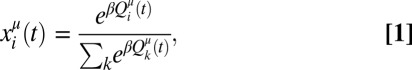where is called the “attraction” for player i to strategy μ. In the special case of experience-weighted attraction that we mainly focus on here, Alice’s attractions are updated according to the following:

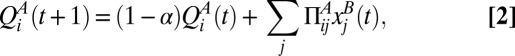and similarly for Bob with A and B interchanged.

Under this update rule, Alice knows her own payoffs and also knows the frequency with which Bob makes each of his possible moves (and similarly for Bob). This approximates the situation in which the players vary their strategies slowly in comparison with the timescale on which they play the game, so that Alice can collect good statistics about Bob before updating her strategy. In the machine learning literature, the practice of infrequent parameter updating is called “batch learning.” We prefer to focus on batch learning because in the large batch limit the dynamics for updating the strategies x^μ of the two players are deterministic, which allows us to compute many properties of the games analytically. The alternative is “online learning,” in which each player updates strategies after every move. Because the moves are randomly chosen, this implies the learning dynamics have a stochastic component. In SI Appendix, section V, we present numerical simulations that show that, with a few exceptions, batch learning and online learning behave similarly, and the main results of the paper hold for both cases.

The key parameters that characterize the learning strategy are α and β. The parameter β is called the intensity of choice; when β is large, a small historical advantage for a given move causes that move to be very probable, and when β = 0, all moves are equally likely. The parameter α specifies the memory in the learning; when α = 1, there is no memory of previous learning steps, and when α = 0, all learning steps are remembered and are given equal weight, regardless of how far in the past. The case α = 0 corresponds to the much-studied replicator dynamics used to describe evolutionary processes in population biology (15–17), where is the concentration of species i in population μ (SI Appendix, section II).

II. Why Investigate Random Games?

Our goal here is to characterize the typical behavior one expects a priori when the strategy for playing a game is learned under reinforcement learning. We first describe what we do, and then explain why we think it is useful.

We construct members of an ensemble of games at random subject to constraints. The constraints we use are that the payoffs have zero mean and a given positive variance, and the payoff to Alice has a given correlation to the payoff to Bob. In mathematical terms, this means that , , and , where E[x] denotes the average of x. Conforming to previous work involving random dynamical systems (3–6, 18), we draw the payoff matrices from a multivariate normal distribution. This was previously presented as an arbitrary choice. In fact, the principle of maximum entropy, which is the foundation of statistical mechanics (19, 20) and has many practical applications in signal processing and machine learning (21), dictates that this is the natural choice, as it is the one that maximizes entropy subject to the above constraints.

The variable Γ is a crucial parameter that measures the correlation in the payoffs of the two players. When Γ = −1 the game is zero sum, i.e., the amount Alice wins is equal to the amount Bob loses, whereas when Γ = 0 their payoffs are uncorrelated, and when Γ = 1 their payoffs are identical. Thus, Γ can be regarded as a competition parameter, where smaller values of Γ indicate more competition.

What can we learn by studying randomly generated games? This depends on whether or not the ensemble of randomly generated games that we have constructed has characteristics that are representative of the “real” games that naturally occur in biology and social science. Can real games be regarded as typical members of the ensemble of random games satisfying the above constraints? If so, then we can obviously learn a great deal by studying the properties of the ensemble. For example, in SI Appendix, see our discussion of 2 × 2 games under replicator dynamics (SI Appendix, section II).

However, what if it turns out that randomly generated games as we generate them here are not representative of real games? In this case, our approach is still valuable as a null hypothesis that can be used to sharpen understanding of what makes real games special. In this case, we would seek alternative constraints leading to alternative ensembles more representative of real games.

For example, if the variance of the payoffs of real games were typically unbounded (which we doubt), this would suggest that the payoffs should be drawn instead from a heavy-tailed Levy distribution, which is the maximum entropy solution in this case. Or there might be additional constraints characterizing biological and social systems that have so far not been identified, which would modify the payoff distribution. Understanding such constraints would obviously be very illuminating, in that it would require discovering new general principles about the generic nature of strategic interactions in real contexts.

An example of work in a similar spirit is the 1972 paper of Robert May (18), which analyzed the generic stability properties of differential equations modeling predator–prey interactions with random coupling coefficients. This work challenged the conventional wisdom that more complex ecosystems are necessarily more stable than simple ones by showing that for a particular ensemble of random equations the opposite is true. The question of whether complex ecosystems are more or less stable remains controversial. In any case, May’s paper has played a vital role by focusing the debate and forcing ecologists to think carefully about the generic properties of ecological interactions. Our intent is similar. Even if it turns out that we are wrong, explaining why we are wrong will hopefully stimulate game theorists to think more carefully about the generic properties of real games.

The characterization of turbulence in fluid mechanics provides a success story analogous to the one we are seeking. The Reynolds number is the ratio of inertial forces to viscous forces in a fluid flow. Based on a very simple analysis, the Reynolds number provides an a priori estimate of whether a fluid flow is likely to be turbulent, and if so, how turbulent it will be. This estimate is crude and inaccurate, but nonetheless very useful. Similarly, our long-term goal is to predict the qualitative nature of the long-term dynamics of a complicated game based on a very cursory analysis of its parameters; we have begun that project by studying a particular ensemble of random games under reinforcement learning.

III. Phase Diagram

We simulate randomly constructed games with n = 50 possible moves, corresponding to a 98-dimensional state space (there are two 50-dimensional strategy vectors and two probability constraints). Roughly speaking, we observe three regimes, as illustrated in the phase diagram of Fig. 1.

• i) “Unique fixed point”: For large values of α and small values of Γ, roughly the lower right triangle in the phase diagram, the learning dynamics x^μ(t) converge to a unique stable fixed point.

• ii) “Multiple fixed points”: In the remainder of the phase diagram with Γ > 0, we observe multiple fixed points. In this case, the multiplicity of the fixed points is often high, e.g., more than 100.

• iii) “Chaos or limit cycle”: For Γ negative and α small, roughly the lower left triangle in the phase diagram, the learning dynamics tend to converge to limit cycles or chaotic attractors, although occasionally we observe other behaviors discussed below.

Fig. 1.

Schematic illustration of the qualitative nature of the asymptotic learning dynamics in the parameter space for complicated random games. β = 0.07.

IV. Characterizing Multiple Attractors and Chaos

For regime (i), in which we observe unique fixed points, there is not much to say about the asymptotic behavior of the learning trajectories x^μ(t): A fixed point is a fixed point. For the other two regimes, however, it is interesting to investigate how the number of stable fixed points varies with parameters in regime (ii) and how the dimensionality of the attractors varies with parameters in regime (iii).

Regime (ii), Multiple Fixed Points.

In regime (ii), we observe multiple stable fixed points depending on initial conditions. A crude survey of the behavior in this region is given in SI Appendix, section IVC. The number of fixed points can be quite high. The most complicated behavior is observed for small values of α and values of Γ near 1. In this case, we typically observe more than 100 fixed points. We want to emphasize that the problem of counting the number of fixed points is difficult, and we cannot be sure that our answers are exact. However, we believe that our results are good enough to accurately indicate the variation between different parts of the parameter space.

Regime (iii), Limit Cycles and Chaos.

We give several examples of the observed learning dynamics at different parameter values in regime (iii) in Fig. 2. These include a limit cycle and chaotic attractors of varying dimensionality. There can also be long transients in which the trajectory follows a complicated orbit for a long time and then suddenly collapses into a fixed point. In general, the behavior observed depends on the random draws of the payoff matrices —the outcomes vary from realization to realization, but if the system is self-averaging then in the limit of large N one expects the behavior to become more and more consistent.

Fig. 2.

An illustration of complex learning dynamics showing trajectories of the strategy x^μ(t) for four different sets of parameters (varying from Left to Right). For each parameter set, we show a phase plot on top and a time series below. For the phase plots, we project the 98-dimensional dynamics onto two dimensions, and we show three representative time series, corresponding to a particular choice of the player and actions. For clarity, we use logarithmic scale. The estimates for the attractor dimensions are obtained as explained in SI Appendix, section IV. As the dimension of the attractor increases, so does the range of . For the highest dimensional case, a given move has occasional bursts where it is highly probable, and long periods where it is extremely improbable (as low as 10⁻⁷²). β = 0.07 in all panels.

To characterize the local stability properties of the attractors, we numerically compute the Lyapunov exponents λ_i, i = 1,…, 2N − 2, which quantify the rate of expansion or contraction of nearby points in the state space. The Lyapunov exponents also determine the Lyapunov dimension D, which measures the number of degrees of freedom of the motion on the attractor.

Simulating games at many different parameter values gives the stability diagram shown in Fig. 3. Roughly speaking, we find that the dynamics are stable when Γ is strongly negative (nearly zero-sum games) and α is large (short memory), i.e., in the lower right of the diagram.* They are unstable when Γ is not too close to zero-sum behavior (imperfectly correlated payoffs) and α is small (long memory). Interestingly, for reasons that we do not understand, the highest dimensional behavior is observed when the payoffs are moderately anticorrelated (Γ ∼ −0.6) and when players have long memory (α ∼ 0). In this regime, we also encounter numerical problems due to the extreme nonlinearities associated with fixed points near the edges of the simplex, and in some cases the dimension is hard to compute reliably.

Fig. 3.

Stability diagram showing where stable vs. chaotic learning is likely when Γ < 0. The colored squares represent the typical dimension of the attractor observed in our simulations (averaged over 10 or more independent payoff matrices at each grid point). White indicates fixed points, pink indicates limit cycles, and yellow indicates high-dimensional chaotic attractors. The solid line is the stability boundary estimated using path-integral methods. β = 0.07.

A good approximation of the boundary between the stable and unstable regions of the parameter space can be computed analytically using techniques from statistical physics. We use path-integral methods from the theory of disordered systems (5, 22) to compute the stability in the limit of infinite payoff matrices, N → ∞. We do this in a continuous-time limit where, for fixed Γ, stability then depends only on the ratio α/β (SI Appendix, section III). The results of doing this are illustrated by the solid black line in Fig. 3, which gives a good approximation for the stability boundary.

We have not yet extensively studied the behavior as N is varied. If D > 0 at small N, then we expect the dimension D to increase with N. At this stage, we have been unable to tell whether D reaches a finite limit or grows without bound as N → ∞.

V. Clustered Volatility and Heavy Tails

An interesting property of this system is the time dependence of the received payoffs. As shown in Fig. 4, when the dynamics are chaotic the total payoff to all of the players varies, with intermittent bursts of large fluctuations punctuated by relative quiescence. This is observed, although to varying degrees, throughout the chaotic part of the parameter space. There is a strong resemblance to the clustered volatility observed in financial markets, which in turn resembles the intermittency of fluid turbulence (12, 23). Financial markets are in fact multiplayer games; our preliminary studies of multiplayer games suggest that these effects become even stronger, and that most parameters lead to chaotic learning dynamics.

Fig. 4.

Chaotic dynamics display clustered volatility. We plot the difference of payoffs on successive time steps for parameter values corresponding to the third panel from the left in Fig. 2. The amplitude of the fluctuations increases with the dimension of the attractor.

Similarly, we also typically observe heavy tails in the distribution of the fluctuations, as shown in SI Appendix, section IVD. The tails that we observe here are exponential, and not power law; we believe this is due to the fact that α sets a fixed timescale. We conjecture that if this timescale is allowed to vary, or in situations with more players with a broad distribution of learning timescales, power law tails may be observed.

The fact that this behavior occurs generically and more or less automatically suggests that these properties, which have received a great deal of attention in studies of financial markets, may occur simply because they are generic properties of the learning dynamics of complicated games.^† Understanding and more thoroughly characterizing this will have to wait for a broader study including a variety of different learning algorithms.

VI. Why Is Dimensionality Relevant?

The fact that the learning dynamics do not converge to an equilibrium under a particular learning algorithm, such as reinforcement learning, does not in general imply that convergent learning might not happen with another algorithm. High dimensionality is relevant because it indicates that the learning dynamics are effectively random. As we explain below, this means that there is no obvious alteration in the learning algorithm of a given player that will improve that player’s performance.

In contrast, if the learning dynamics settle into a limit cycle or a low dimensional attractor, Alice could collect data and make better predictions about Bob’s likely decisions using the method of analogs (24) or refinements based on local approximation (25). Assuming Bob does not alter his strategy, and assuming the dynamics are sufficiently stable under variations in parameters, Alice could use her predictions to make small alterations in her strategy so as not to alter the combined learning dynamics of the two players too much, thereby perturbing the system onto a nearby attractor and improving her average payoff.

If the dimension of the chaotic attractor is too high, however, the curse of dimensionality makes this impossible with any reasonable amount of data (25). Thus, high dimensionality indicates that the chaotic attractors we observe here are rather complicated Nash equilibria, in the sense that there are no easily learnable superior strategies nearby.

This raises the question of whether there are games where learning will fail to cause the strategies to converge to a fixed point under any inductive learning algorithm. The observation of high-dimensional chaos adds weight to the suggestion that there are. The existence of such high-dimensional chaos is reminiscent of the ergodic conjecture of statistical mechanics, which loosely speaking says that for many nonlinear dynamical systems almost all of the trajectories display high-dimensional chaos, and consequently can only be characterized by statistical averages. See also refs. 14, 26, and 27.

VII. Concluding Discussion

Our work here indicates that for games drawn from the ensemble that we describe here, it is possible to characterize the learning dynamics under experience-weighted attraction a priori. We have shown that a key property of such games is their competitiveness, characterized by the parameter Γ. Games become harder to learn (in the sense that the strategies do not converge to a fixed point) when they are more competitive, i.e., closer to being zero sum, particularly if the players use learning algorithms with long memory. This analysis can potentially be extended to multiplayer games, games on networks, alternative learning algorithms, etc.

Comparison with behavioral experiments modeled with experience-weighted attraction as reported in ref. 7 shows that the parameters we are using here are roughly within the range observed in real experiments. Values for memory-loss parameters and intensity of choice reported from experiments suggest that real-world decision making may well operate near or in the chaotic phase (SI Appendix, section I). Most experimental data are limited to games with only a few moves, however, whereas here we study games with a large number of possible moves.

Our study here only begins to scratch the surface of what might potentially be learned from this general line of investigation. To draw more general conclusions, studies of a wide variety of learning algorithms are needed, and one would like to repeat such analysis for broader classes of games. Our preliminary studies of multiperson games, for example, indicate that as the number of players increases the chaotic regime grows, and in the limit where the number of players becomes large, chaos becomes dominant. Our work also suggests that many behaviors that have attracted considerable interest, such as clustered volatility and heavy tails observed in financial markets, may simply be specific examples of a highly generic phenomenon, and should be expected to occur in a wide variety of different situations.

References

- 1.Nash JF. Equilibrium points in n-person games. Proc Natl Acad Sci USA. 1950;36(1):48–49. doi: 10.1073/pnas.36.1.48. [DOI] [PMC free article] [PubMed] [Google Scholar]
- 2.von Neumann J, Morgenstern O. Theory of Games and Economic Behaviour. Princeton: Princeton Univ Press; 2007. [Google Scholar]
- 3.McLennan A, Berg J. The asymptotic expected number of Nash equilibria of two player normal form games. Games Econ Behav. 2005;51(2):264–295. [Google Scholar]
- 4.Berg J, Weigt M. Entropy and typical properties of Nash equilibria in two-player Games. Europhys Lett. 1999;48(2):129–135. [Google Scholar]
- 5.Opper M, Diederich S. Phase transition and 1/f noise in a game dynamical model. Phys Rev Lett. 1992;69(10):1616–1619. doi: 10.1103/PhysRevLett.69.1616. [DOI] [PubMed] [Google Scholar]
- 6.Diederich S, Opper M. Replicators with random interactions: A solvable model. Phys Rev A. 1989;39(8):4333–4336. doi: 10.1103/physreva.39.4333. [DOI] [PubMed] [Google Scholar]
- 7.Ho TH, Camerer CF, Chong J-K. Self-tuning experience weighed attraction learning in games. J Econ Theory. 2007;133:177–198. [Google Scholar]
- 8.Camerer C, Ho TH. Experience-weighted attraction learning in normal form games. Econometrica. 1999;67:827. [Google Scholar]
- 9.Camerer C. Behavioral Game Theory: Experiments in Strategic Interaction (The Roundtable Series in Behavioral Economics) Princeton: Princeton Univ Press; 2003. [Google Scholar]
- 10.Fudenberg D, Levine DK. Theory of Learning in Games. Cambridge, MA: MIT Press; 1998. [Google Scholar]
- 11.Young HP. Individual Strategy and Social Structure: An Evolutionary Theory of Institutions. Princeton: Princeton Univ Press; 1998. [Google Scholar]
- 12.Brock WA, Hommes CH. Heterogeneous beliefs and routes to chaos in a simple asset pricing model. J Econ Dyn Control. 1998;22:1235–1274. [Google Scholar]
- 13.Skyrms B. Chaos in game dynamics. J Log Lang Inf. 1992;1:111–130. [Google Scholar]
- 14.Sato Y, Akiyama E, Farmer JD. Chaos in learning a simple two-person game. Proc Natl Acad Sci USA. 2002;99(7):4748–4751. doi: 10.1073/pnas.032086299. [DOI] [PMC free article] [PubMed] [Google Scholar]
- 15.Sato Y, Crutchfield J-P. Coupled replicator equations for the dynamics of learning in multiagent systems. Phys Rev E 67. 2003 doi: 10.1103/PhysRevE.67.015206. 015206(R) [DOI] [PubMed] [Google Scholar]
- 16.Nowak MA. Evolutionary Dynamics. Cambridge, MA: Harvard Univ Press; 2006. [Google Scholar]
- 17.Hofbauer J, Sigmund K. Evolutionary Games and Population Dynamics. Cambridge, MA: Cambridge Univ Press; 1998. [Google Scholar]
- 18.May RM. Will a large complex system be stable? Nature. 1972;238(5364):413–414. doi: 10.1038/238413a0. [DOI] [PubMed] [Google Scholar]
- 19.Jaynes ET. Information theory and statistical mechanics. Phys Rev. 1957;106:620–630. [Google Scholar]
- 20.Jaynes ET. Information theory and statistical mechanics II. Phys Rev. 1957;108:171–190. [Google Scholar]
- 21.Cover TM, Thomas JA. Elements of Information Theory. 2nd Ed. Hoboken, NJ: Wiley-Interscience; 2006. [Google Scholar]
- 22.De Dominicis C. Dynamics as a substitute for replicas in systems with quenched random impurities. Phys Rev B. 1978;18:4913–4919. [Google Scholar]
- 23.Ghashghaie S, Breymann W, Peinke J, Talkner P, Dodge Y. Turbulent cascades in foreign exchange markets. Nature. 1996;381:767–770. [Google Scholar]
- 24.Lorenz EN. Atmospheric predictability revealed by naturally occurring analogues. J Atmos Sci. 1969;26:636–646. [Google Scholar]
- 25.Farmer JD, Sidorowich JJ. Predicting chaotic time series. Phys Rev Lett. 1987;59(8):845–848. doi: 10.1103/PhysRevLett.59.845. [DOI] [PubMed] [Google Scholar]
- 26.Foster DP, Young HP. On the impossibility of predicting the behavior of rational agents. Proc Natl Acad Sci USA. 2001;98(22):12848–12853. doi: 10.1073/pnas.211534898. [DOI] [PMC free article] [PubMed] [Google Scholar]
- 27.Hart S, Mas-Colell A. Uncoupled dynamics do not lead to Nash equilibrium. Am Econ Rev. 2003;93(5):1830–1836. [Google Scholar]
Associated Data
This section collects any data citations, data availability statements, or supplementary materials included in this article.