Two-stage Extreme Phenotype Sequencing Design for Discovering and Testing Common and Rare Genetic Variants: Efficiency and Power

Abstract

Next-generation sequencing technology provides an unprecedented opportunity to identify rare susceptibility variants. It is not yet financially feasible to perform whole-genome sequencing on a large number of subjects, and a two-stage design has been advocated to be a practical option. In stage I, variants are discovered by sequencing the whole genomes of a small number of carefully selected individuals. In stage II, the discovered variants of a large number of individuals are genotyped to assess association. Individuals with extreme phenotypes are typically selected in stage I. Using simulated data for unrelated individuals, we explore two important aspects of this two-stage design: the efficiency of discovering common and rare single-nucleotide polymorphisms (SNPs) in stage I and the impact of incomplete SNP discovery in stage I on the power of testing associations in stage II. We apply a sum test and a sum of squared score test for gene-based association analyses evaluating the power of the two-stage design. We obtained the following results from extensive simulation studies and analysis of the GAW17 dataset. When individuals with trait values more extreme than the 99.7 to 99^th quantile are included in stage I, the two-stage design could achieve the same as or even higher power than one-stage design if the rare causal variants have large effect sizes. In such tests, fewer than half of the total SNPs including more than half of the causal SNPs were discovered, which included nearly all SNPs with minor allele frequencies (MAFs) ≥ 5%, more than half of the SNPs with MAFs between 1% and 5%, and fewer than half of the SNPs with MAFs <1%. Although a one-stage design may be preferable to identify multiple rare variants having small to moderate effect sizes, our observations support using the two-stage design as a cost-effective option for next-generation sequencing studies.

Introduction

Common single-nucleotide polymorphisms (SNPs) that are associated with complex traits explain only a small proportion of the genetic component of the trait variation. Recently, evidence has been emerging that less common (minor allele frequency [MAF], 1% to 5%) and rare variants (MAF <1% but still polymorphic) contribute to the risk of complex diseases such as autism, epilepsy, and schizophrenia [1]. State-of-the-art, next-generation sequencing technology provides an unprecedented opportunity for identifying less common and rare variants having modest to large effect sizes. Currently, it is still expensive to perform whole-genome sequencing in large samples such as those used in genome-wide association (GWA) studies. Toward this end, two types of two-stage designs have been proposed as practical options to balance cost and power [2–5]. Both involve a stage of variant discovery via whole-genome sequencing (stage I) and a stage of association testing in much larger, independent samples for which the stage I variants are genotyped (stage II). One design involves sequencing a moderate number of pooled samples [3–4], and the other involves sequencing a small number of individuals with extreme phenotype values [5]. We focus on the second study design in this paper and call it “two-stage extreme phenotype sequencing design” (TS-E).

Guey et al. [6] found that using individuals with extreme phenotypes could lead to high efficiency for discovering rare variants in stage I but limited power for detecting associations. They estimated power based on testing a single rare variant and did not compare the power of the TS-E or one-stage design in which the whole genomes of all individuals are sequenced. Here, through extensive simulation studies and analysis of GAW 17 mini-exome data [7], we comprehensively examine the efficiency of SNP discovery in stage I and compare the overall power of TS-E to identify susceptible gene regions to that of the one-stage design.

Our results supported the feasibility of the TS-E. It may fail to discover a large proportion of rare variants, but such incomplete variant discovery may not translate into decreased power for identifying genetic regions that harbor causal variants if causal variants are common or if they are rare but have large effect sizes. This observation is largely because a smaller number of non-causal variants are discovered in stage I in the TS-E than in the one-stage design. In our simulation studies, when more than 10 subjects were selected in stage I for discovering variants, the two-stage design achieved nearly the same power as did the one-stage design. On the other hand, if one seeks to identify multiple rare variants having small or moderate effect sizes, then a one-stage design may be preferable. Our results provide guidance for designing a two-stage study that balances the power and cost given the total number of stage I and II individuals.

Method

To implement the TS-E in our simulation studies, we first generated 20 000 SNPs in 200 gene regions for every individual, which are assumed to be the complete exome sequencing data and are referred to as the mini-exome data. Among the 20 000 SNPs, some SNPs with MAFs < 0.05 were assumed to be causal and had moderate to large effect sizes, and a few common SNPs (MAFs ≥ 0.05) were assumed to be causal and had small to moderate effect sizes. We then generated values for a quantitative trait from a linear regression model. In addition, we analyzed 200 simulated mini-exome and quantitative trait datasets of 697 unrelated individuals from the Genetic Analysis Workshop 17 (GAW17).

Stage I: SNP Discovery by Sequencing Individuals with Extreme Phenotypes

Denote y_l and y_u as the lower l and upper u = 1 − l quantiles of trait Y for m independent individuals from a homogeneous population. Individuals satisfying Y ≥ y_u or Y ≤ y_l are selected for sequencing. We treat the SNPs whose estimated MAFs in the selected individuals are greater than zero as the “discovered SNPs”. We deem a gene as a “discovered gene” if at least 1 SNP within this gene is discovered. In keeping with Cirulli and Goldstein’s [5] categorization of potential causal variant frequencies, we classify the discovered SNPs (MAFs > 0) into three groups: common variants (CVs; MAFs, 5%–50%), less common variants (LCVs; MAFs, 1% – 5%), and rare variants (RVs; MAFs, < 1%). To fully understand the merit of TS-E, we also evaluated the efficiency of an alternative two-stage design in which stage I individuals are selected randomly: We refer to this design as TS-R.

Suppose that the discovered SNPs are genotyped for the remaining (1 − 2l)m individuals in stage II. Let T_w and T_s denote the respective costs of sequencing and genotyping discovered SNPs for 1 individual. We assume that T_s is the same for genotyping different numbers of discovered SNPs when calculating the cost benefit. The cost fraction 2l + (1 − 2l) T_s/T_w represents the relative cost of the two-stage design compared with the one-stage design in which all m individuals are sequenced. For example, with l = 0.005 and T_s/T_w = 0.5, the cost fraction is 0.51. This cost fraction translates into a 49% reduction in the total cost.

Stage II: Gene-based Association Testing based on Discovered SNPs

We subsequently assessed the association between each gene and a particular phenotype by using the discovered SNPs for subjects in Stage II, aiming to evaluate the impact of incomplete SNP discovery in stage I on the power of stage II association testing. We applied 2 gene-based association testing methods: the simple modified sum test, which is one of the most powerful methods when effects of the causal variants have the same direction and there are no or few non-causal RVs, and the sum of squared score test (SSU), which is one of the most powerful tests in the presence of opposite association directions and non-causal RVs [8]. Both the sum test and SSU yielded a p-value for the significance of each gene rather than for that of each SNP. Testing each gene rather than each SNP is in line with the current wisdom.

The sum test

Suppose that observations (Y_i, X_i) are available for N individuals, i=1, 2, …, N, where Y_i is the value of a quantitative trait for subject i and X_i = (X_i1, .., X_iK)^T is the vector of minor allele counts (0, 1, 2) for the K SNPs within the tested gene region for the same subject. A tested gene region includes all SNPs within 20 kb of the start and stop of the gene [9]. Let K₁, K₂, and K₃ = K − K₁ − K₂ be the respective numbers of CV, LCV, and RV within the tested gene region. By adapting the combined multivariate and collapsing (CMC) method [10] and the sum test [7] to accommodate both rare and common variants, we use a linear regression model to describe the association between the trait Y and the K SNPs,

$$Y_i={\beta }_0+{\beta }_1\sum _{j=1}^{K_1}\frac{X_{ij}^{cv}}{K_1}+{\beta }_2\sum _{j=1}^{K_2}\frac{X_{ij}^{\mathit{lcv}}}{K_2}+{\beta }_3\sum _{j=1}^{K_3}\frac{X_{ij}^{rv}}{K_3}+{\epsilon }_i,$$ (1)

where ε_i is the random error term that follows the standard normal distribution and superscripts cv, lcv, and rv represent CV, LCV, and RV within this gene, respectively. We divide the summation of minor allele counts by the number of SNPs to account for different numbers of SNPs within each category. We test the null hypothesis of no association between the gene and the trait by testing the null hypothesis β₁ = β₂ = β₃ = 0 with the standard likelihood ratio statistic. For association tests in the two-stage design, only the discovered SNPs within each gene are included in the model.

The sum of squared score test (SSU)

In the presence of opposite association directions and non-causal RVs, the SSU is one of the most powerful tests for detecting rare variants [7]. It is reasonable that it would also be powerful for testing common and rare variants jointly because it is robust to the number of parameters for multiple genetic variants. Under a linear regression model for the association between the trait Y and the K SNPs,

$$Y_i={\beta }_0+\sum _{j=1}^K{X}_{ij}{\beta }_j,$$

the SSU statistic, T_SSU, is equal to U^TU, where $U={\sum }_{i=1}^N(Y_i-\overline{Y})X_i$ and $\overline{Y}={\sum }_{i=1}^N\frac{Y_i}{N}$. Under the null hypothesis of no association, β_j = 0, j = 1, 2, … K, T_SSU asymptotically follows a distribution of a mixture of ${\chi }_1^2$’s that can be approximated by a scaled and shifted Chi-squared distribution [8]. Here, we used the permutation re-sampling method to estimate the empirical p-values of the SSU test.

Simulation studies

We assessed the efficiency of discovering both common and rare SNPs, the type-I error rate, and the power of the two-stage design, assuming that multiple common and rare variants could be associated with a quantitative trait.

Generating genotype data based on linkage disequilibrium (LD)

We generated SNP genotype data directly rather than generating raw sequencing reads [10–13]. To ensure that there were more rare variants than common ones, we first generated MAFs for 20 000 SNPs from the Wright’s distribution [14–15], similar to Ionita-Laza et al. [13], Pritchard [14], and Madsen and Browning [15]. This distribution has the density function f(p) = cp^{β_s − 1}(1 − p)^{β_n − 1}e^{σ(1 − p)}, where β_s and β_n are the scaled mutation rates and were set at values 0.001 and 0.001/3, respectively; σ is the selection rate and was set at 12, and c is the normalizing constant. We then generated mini-exome genotype data for 2000 unrelated individuals in 3 steps by controlling pair-wise LD values [11–12]. First, we generated 4000 latent vectors, each of length 20 000, (W_j1, W_j2, …, W_j20,000), where j indicates the j-th vector. Each latent vector is generated from a multivariate normal distribution with a first-order, auto-regressive covariance structure, where the correlation between the lth and kth component of the jth vector is corr(W_jl, W_jk) = ρ^ll−k|. Different values of ρ correspond to different levels of LD, with ρ = 0 indicating linkage equilibrium (LE) and greater ρ indicating stronger LD between neighboring variants. LD between common and rare variants and among rare variants is generally weak [16–17], but LD among common variants could be strong. We, therefore, considered 2 different LD structures among all CVs and LCVs: (1) the CVs and LCVs are in linkage equilibrium (ρ = 0); (2) the CVs and LCVs are situated in regions of moderate LD (ρ = 0.5). All of the RVs were in LE. Next, each latent vector was dichotomized to construct a haplotype (H_j1, H_j2, …, H_j20,000) where H_jk represents the allele at the kth locus that takes a value of 0 for the major one or a value of 1 for the minor one. Lastly, we combined 2 haplotypes at random to form an individual’s genotype data (X_i1, .., X_i20000), where X_ik is equal to the summation of H_jk’s in the 2 haplotypes. The final data for analysis contained 1761 (8.8%) CVs, 4167 (20.8%) LCVs, and 14 072 (70.4%) RVs. The distribution of the allele frequencies of 20 000 SNPs was similar to that of the GAW17 data (Supplementary Figure S1).

Generate phenotype data

We randomly selected k SNPs from the first gene as the causal SNPs. We then generated a quantitative trait Y for each individual from the linear model: $Y_i={\beta }_0+{\sum }_{j=1}^k{X}_{ij}{\beta }_j+e_i$, where e_i is the random error term following the standard normal distribution, and β is the vector of regression coefficients, with β = 0 indicating no association. We considered 5 models of association. The first 4 models had 7 causal variants (k = 7), including 2 CVs, 1 LCV, and 4 RVs, and they differed only in the magnitude and direction of β coefficients for the 7 variants. The fifth model had 20 causal variants, including 3 CVs, 3 LCVs, and 14 RSs [18]. The model parameters were chosen to ensure that the phenotype variability explained by LCVs and RVs was more than that explained by CVs. The MAFs, effect sizes, and percentage of explained phenotype variability are provided in Supplementary Tables S1 and S2.

Efficiency of stage I SNP discovery, type I error rate, and power

To evaluate the merits of the TS-E using the gene-based association tests, we varied the proportion of individuals included in step I SNP discovery (l) from 0.001 to 0.02 at an increment of 0.0015. For stage I SNP discovery, we presented the average percentages of the total discovered SNPs, the discovered CVs, the discovered LCVs, the discovered RVs, and the discovered causal SNPs across 1000 replicates. For comparison, we presented the stage I SNP discovery results of both TS-E and TS-R under each of the 5 association models. For stage II gene-based association tests using discovered SNPs, we included only stage II subjects in the sum test to evaluate its power because including stage I subjects in association testing may inflate the type I error rate of the sum test [10, 24]. But we included all samples in the SSU test because we used the permutation re-sampling method to obtain the empirical p-value. We controlled the overall type I error rate at the nominal level (0.05) by applying the Bonferroni method. We also evaluated the power of TS-R for models 1 and 2 when all SNPs were in LE. To assess the impact on power of using only discovered SNPs for association testing, we also reported the corresponding power of the one-stage design.

Results

Stage I SNP discovery

Figure 1 shows results for stage I SNP discovery and the corresponding cost reduction when all SNPs are in LE. The TS-E discovered nearly the same percentages of total SNPs, CVs, LCVs, and RVs as did TS-R, regardless of the penetrance models (Figures 1A–1E) and LD structure (Supplementary Figures S2A–S2E). However, as expected, TS-E discovered a much higher percentage of the causal SNPs than did TS-R with the same proportion of stage I individuals (Figures 1F–1J) in all scenarios (Supplementary Figures S2F–S2J). With 2l = 0.02 of subjects included in stage I, the respective percentages of discovered total SNPs, CVs, LCVs, and RVs by both TS-E and TS-R were 36%, 100%, 80%, and 15% (Figure 1A). But the percentages of discovered causal SNPs were 77.8% by TS-E and 47.6% by TS-R (Figure 1B). These results are consistent with those in the literature [19] and are also consistent with the conventional wisdom that TS-E is more cost-effective than TS-R is for designing next-generation sequencing projects.

Figure 1. SNP discovery in stage I when all SNPs are in LE and the cost reduction of the two-stage designs based on simulation data.

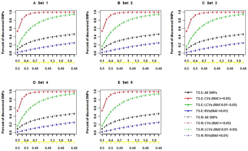
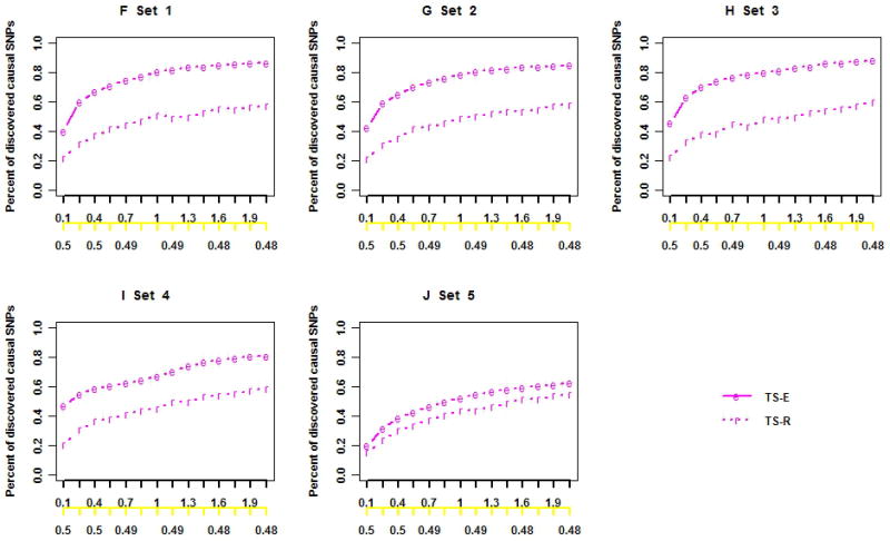
The black x-axis is the proportion of stage I individuals times 100 (l × 100), and the yellow x-axis is the cost function with T_s/T_w = 0.5. The black, red, green, blue, and pink lines indicate the percentages of the total discovered SNPs, CVs, LCVs, RVs, and causal SNPs, respectively. Letters “e” and “r” indicate two-stage designs with extreme phenotype sampling (TS-E) or random sampling (TS-R), respectively.

Not surprisingly, the percentages of discovered total SNPs, CVs, LCVs, RVs, and causal SNPs increased with the proportion of stage I individuals, and the increases were sharp when the phase I proportion was small (Figures 1A–1J and Supplementary Figures S2A–S2J). With l increasing from 0.001 to 0.007, the respective percentages of discovered total SNPs, CVs, LCVs, and causal SNPs increased from 10% to 31%, 54% to 99%, 17% to 69% (Figure 1A), and 40% to 73% (Figure 1F). But the percentage of discovered rare SNPs hardly increased: it was as low as 25%, even when 2% were included in stage I (Figure 1A). The percentage of discovered causal SNPs varied greatly with the association models. If the causal LCVs and RVs had large effects (Figures 1F–1I), then TS-E appeared to be much more efficient for discovering causal variants than TS-R did. With TS-E, more than 60% of the causal variants can be discovered when l=0.004 (ie, 16 subjects were included in Stage I), and 80% can be discovered when l=0.02 (ie, 80 subjects were included in Stage I). When the genetic variability of the phenotype was mostly due to multiple LCVs and RVs having small or moderate effect sizes, less than 60% of the causal SNPs were discovered, even with l=0.02, and TS-E and TS-R appeared to have similar efficiency for discovering causal variants (Figure 1J). In general, the LD structure among common SNPs and the presence or absence of opposite association directions had a minor effect on SNP discovery (Figure 1A–1D and Supplementary Figure S2A–S2D).

Type I error rate and power

The type I error rates of the sum test and SSU test for analyzing TS-E, TS-R, and one-stage designs appeared to be close to the nominal level (0.05), regardless of whether SNPs were in LE (Table 1) or in LD (Supplementary table S3). We first compared the power of the sum test and SSU test for analyzing joint effects of both common and rare variants under the 5 association models we considered. We then compared the power of the 3 designs (TS-E, TS-R, and one-stage design) by using the 2 tests under the 5 models. Figures 2A–E and Supplementary Figures S3 A–E show that power was at the nominal level of 0.05 when all SNPs were in LE (LD). Under the one-stage design, the SSU test had much higher power than did the sum test if the total number of causal variants was small and the causal LCVs and RVs had large effect sizes (Figures 2A–2D and Supplementary Figures S3A–S3D). But the sum test had higher power when the causal variants consisted of a large number of LCVs and RVs with a common small effect size (Figure 2E and Supplementary Figure S3E).

Figure 2. The power of TS-E under the 5 disease models when all SNPs are in LE based on 1000 sets of simulated data.

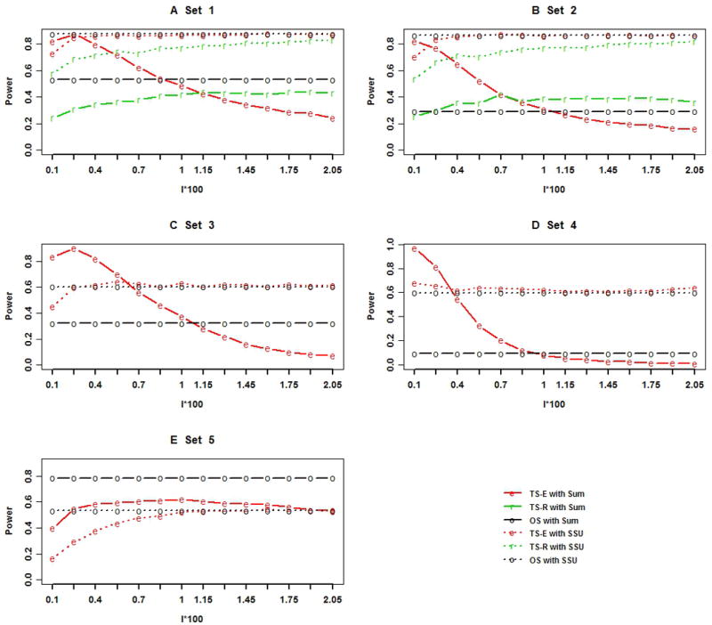
The black x-axis is the proportion of stage I individuals times 100 (l × 100). Solid black line with letter “o”: one-stage design using the sum test; Solid red line with letter “e”: the two-stage design with extreme phenotype sampling (TS-E) using the sum test; Solid green line with letter “r”: the two-stage design with random sampling (TS-R) using the sum test; Dashed black line with letter “o”: one-stage design using the sum of squares (SSU) test; Dashed red line with letter “e”: the TS-E using the SSU test; Dashed green line with letter “r”: TS-R using the SSU test.

Power comparisons of the 3 designs under the sum test

With the sum test used in the stage II association analysis, the power of TS-E was first greater and then smaller than that of the one-stage design and TS-R with the proportion of stage I individuals if the RVs had large effect sizes, regardless of the LD structure among common SNPs (Figures 2A–2D, and Supplementary Figures S3A–S3D). If all of the causal LCVs and RVs had small effect sizes of similar magnitude, then the power of one-stage design was always higher than that of TS-E (Figure 2E and Supplementary Figure S3E). The power difference becomes larger with smaller and larger proportion of stage I individuals regardless of disease models (Figures 2A–2E) and LD structure among CVs and LCVs (Supplementary Figures S3A–S3E). The advantage of the TS-E decreased as the proportion of individuals included in stage I became larger (greater than 0.085 in the simulation study) if the causal RVs had large effect sizes (Figures 2A–2D and Supplementary Figures S3A–S3D). With larger stage I proportion, although most causal variants were discovered, the sample size for stage II association tests became smaller, and even more unassociated SNPs were discovered and included in the association tests in stage II.

Power comparisons of 3 designs under the SSU test

With the SSU test used in the stage II association test, the power of TS-E was nearly identical to that of the one-stage design when more than 10 subjects (l = 0.00025) were selected in Stage I under the first 4 association models. When causal SNPs included CVs (Figure 2A–2B), the power was higher than 90%. When causal SNPs consisted of LCVs and RVs of large effect sizes (Figures 2C–2D), the power was approximately 60%. When the causal SNPs consisted of LCVs and RVs having small effect sizes (Figure 2E), with 10 subjects included in stage I, the power of TS-E was 25%; with 40 subjects included in stage I (l = 0.01), the power of TS-E approached that of the one-stage design. The power of TS-E was generally higher than that of TS-R (Figures 2A–2B), but the difference was smaller when stage I sample size was increased.

Under both the one-stage design and TS-E, it appeared that the SSU test had higher power than did the sum test when the causal variants included LCVs and RVs having large effect sizes (Figures 2A–2D). However, when the causal variants consisted of a relatively large number of LCVs and RVs having small effect sizes, the sum test had higher power than did the SSU test for both one-stage design and TS-E (Figure 2E and Supplementary Figure S3E). Interestingly, the power of the sum test under TS-E could be higher than that of the SSU test under the one-stage design with appropriate proportions of stage I individuals (Figures 2C–2E and Supplementary Figures S3C–S3E).

Application to the GAW17 dataset

We applied the TS-E to the GAW17 dataset of unrelated individuals [7], which contained genotype data of 24 487 SNPs in 3205 genomic regions of 697 unrelated individuals. These SNPs included 3132 CVs, 3224 LCVs, and 18131 RVs. One quantitative trait, denoted as Q₂, was not correlated with any of the 3 covariates provided in the dataset, and 200 replicate datasets for Q₂ were provided based on genotypes of 72 causal SNPs in 13 gene regions. Among the 72 causal SNPs, 2 (2.8%) were CVs, 4 (5.6%) were LCVs, and 66 (91.6%) were RVs. The limited sample size of the GAW17 dataset caused the power for testing associations based on each individual phenotype dataset to be low. Furthermore, the GAW17 used a fixed genotype dataset to generate 200 replicate phenotype datasets, so that the variation in the phenotype data across replicates was due to random error. Therefore, we used the average of the phenotype values in the first 10 datasets, denoted as Q_2–10, as the phenotype for the evaluation of the TS-E. The percentages of the Q_2–10 variance explained by causal CVs, LCVs, and RVs are provided in Supplementary Table S4.

Figure 3 shows the results for stage I SNP discovery using TS-E and the corresponding cost reduction. When subjects in the lower and upper 0.0035 quantiles were selected on the basis of Q_2–10, 17% of the total SNPs were discovered, which included 86% of the CVs, 26% of the LCVs, and 3.3% of the RVs. These results are consistent with those in the literature [19]. In addition, the discovered SNPs included 12.5% of the 72 causal SNPs and 31% (998) of the total number of genes. In particular, 6 of 13 causal genes (BCHE, LPL, PDGFD, SIRT1, VNN1, and VNN3) were discovered in the sense that at least 1 SNP was discovered in each of these gene regions. We observed that either some CVs existed in the gene or that the causal SNPs explained a large proportion of the phenotypic variance.

Figure 3. SNP discovery of the two-stage design with extreme phenotype sampling (TS-E) in the GAW17 data.

The black x-axis is the proportion of stage I individuals times 100 (l × 100), and the yellow x-axis is the cost function with T_s/T_w = 0.5. The black, red, green, blue, and pink lines correspond to the percentage of total discovered SNPs, CVs, LCVs, discovered RVs, and causal SNPs, respectively.

Figure 4 plots the −log₁₀ (p-values) of the sum and SSU tests under TS-E for each of the 13 causal genes. Interestingly, the p-values of the sum test and SSU test for the full dataset (the one-stage design) for the undiscovered causal genes VWF, VLDLR, RARB, PLAT, GCKR, and INSIG1 were similar. For these genes, LCVs and RVs only accounted for a small proportion of the phenotypic variance (supplementary Table S4). For the discovered genes that had causal CVs or causal RVs with relatively large effect sizes [7], such as VNN3, LPL, PDGFD, and VNN1, the p-values of the sum test under both one-stage and TS-E designs were also similar. For the remaining 2 discovered genes, SIRT1 and BCHE, the sum test was not significant under either one-stage or TS-E designs. Both genes contained causal RVs having moderate or small effect sizes. The analysis with the SSU test yielded results similar to those of the sum test.

Figure 4. The − log p-values for the 13 causal genes under the two-stage design with extreme phenotype sampling (TS-E) in the GAW17 data (l=0.0035).

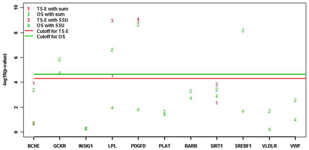
The y-axis is −log₁₀ (p-value). The numbers 1, 2, 3, and 4 respectively correspond to results of TS-E using the sum test, one-stage design using sum test, TS-E using the SSU test, and one-stage design using the SSU test. The green and red lines indicate the cutoffs for the one-stage design and TS-E with l = 0.0035 using Bonferroni correction.

Discussion

Here, we have evaluated the merits of TS-E in assessing both rare and common variants for association. Our results indicate that the stage I sample size is a very important factor for the success of TS-E because it determines the percentage of discovered causal SNPs. If one suspects multiple numbers of susceptibility LCVs or RVs with small or moderate effect sizes, then perhaps a one-stage design should be planned. Sequencing just a small proportion of subjects for SNP discovery may ultimately lead to low power in association studies. However, if one aims to detect rare variants with large effect sizes, then the two-stage design would be a feasible option, as suggested in the literature, and can have the same power as the one-stage design when accompanied by appropriate methods of analysis. In our simulation studies, the TS-E that includes merely the discovered SNPs in the SSU test could achieve nearly the same power as the one-stage design could. The analysis of the GAW17 dataset further confirmed the efficiency of the TS-E for identifying both rare and common variants. In general, as long as rare variants having large effect sizes account for a larger proportion of the phenotypic variance than common variants do, the TS-E should be recommended because it balances statistical power and cost efficiency. We expect that our observations will be useful for those who wish to use TS-E for next-generation sequencing studies.

We only considered 2 methods for analysis in this work, the sum test and the SSU test. When all causal SNPs were positively associated with the trait, the other 2 popular methods of analysis, the CMC test [10] and the weighted sum test [15] have power similar to that of the sum test [8]. When the minor alleles of the causal SNPs may be negatively associated with the trait, the kernel machine regression [20], the C-alpha-P test [21], sequence Kernel Association test method [22], and data-adaptive sum test [23] have power similar to that of the SSU test. Therefore, we expect that the qualitative results we obtained would still hold if other methods had been used for analysis. In addition, we assumed that the stage I and stage II individuals were from a homozygous population. When the study population is less homogeneous, the stage I sample should balance the numbers from different subpopulations.

References

- 1.Stankiewicz P, Lupski JR. Structural variation in the human genome and its role in disease. Ann Rev Med. 2010;61:437–455. doi: 10.1146/annurev-med-100708-204735. [DOI] [PubMed] [Google Scholar]
- 2.Schaid DJ, Sinnwell JP. Two-stage case-control designs for rare genetic variants. Hum Genet. 2010;127:659–68. doi: 10.1007/s00439-010-0811-x. [DOI] [PMC free article] [PubMed] [Google Scholar]
- 3.Bansal V, Tewhey R, LeProust EM, Schork NJ. Efficient and cost effective population resequencing by pooling and in-solution hybridization. PLOS One. 2011;6:e18353. doi: 10.1371/journal.pone.0018353. [DOI] [PMC free article] [PubMed] [Google Scholar]
- 4.Kim SY, Li Y, Guo Y, Li R, Holmkvist J, et al. Design of association studies with pooled or un-pooled next-generation sequencing data. Genet Epidemiol. 2010;34:479–491. doi: 10.1002/gepi.20501. [DOI] [PMC free article] [PubMed] [Google Scholar]
- 5.Cirulli ET, Goldstein DB. Uncovering the roles of rare variants in common disease through whole-genome sequencing. Nature Rev Genet. 2010;11:415–425. doi: 10.1038/nrg2779. [DOI] [PubMed] [Google Scholar]
- 6.Guey LT, Kravic J, Melander O, Burtt NP, Laramie JM, Lyssenko V, Jonsson A, Lindholm E, Tuomi T, Isomaa B, Nilsson P, Almgren P, Kathiresan S, Groop L, Seymour AB, Altshuler D, Voight BF. Power in the phenotypic extremes: a simulation study of power in discovery and replication of rare variants. Genet Epidemiol. 2011;32:236–246. doi: 10.1002/gepi.20572. [DOI] [PubMed] [Google Scholar]
- 7.Blangero J, et al. Genetic Analysis Workshop 17 mini-exome simulation. BMC Proceedings. 2011 doi: 10.1186/1753-6561-5-S9-S2. [DOI] [PMC free article] [PubMed] [Google Scholar]
- 8.Basu S, Pan W. Comparison of statistical tests for disease association with rare variants. Genetic Epidemiology. 2011;35:606–619. doi: 10.1002/gepi.20609. [DOI] [PMC free article] [PubMed] [Google Scholar]
- 9.Purcell S, Neale B, Todd-Brown K, Thomas L, Ferreira MAR, Bender D, Maller J, Sklar P, de Bakker PIW, Daly MJ, Sham PC. PLINK: a toolset for whole-genome association and population-based linkage analysis. American Journal of Human Genetics. 2007;81:559–575. doi: 10.1086/519795. [DOI] [PMC free article] [PubMed] [Google Scholar]
- 10.Li B, Leal SM. Methods for detecting associations with rare variants for common diseases: application to analysis of sequence data. Am J Hum Genet. 2008;83:311–321. doi: 10.1016/j.ajhg.2008.06.024. [DOI] [PMC free article] [PubMed] [Google Scholar]
- 11.Pan W. Asymptotic tests of association with multiple SNPs in linkage disequilibrium. Genetic Epidemiology. 2009;33:497–507. doi: 10.1002/gepi.20402. [DOI] [PMC free article] [PubMed] [Google Scholar]
- 12.Wang T, Elston RC. Improved power by use of a weighted score test for linkage disequilibrium mapping. Am J Hum Genet. 2007;80:353–360. doi: 10.1086/511312. [DOI] [PMC free article] [PubMed] [Google Scholar]
- 13.Ionita-Laza I, Buxbaum JD, Laird NM, Lange C. A new testing strategy to identify rare variants with either risk or protective effect on disease. PLoS Genetics. 2011;7(2):e1001289. doi: 10.1371/journal.pgen.1001289. [DOI] [PMC free article] [PubMed] [Google Scholar]
- 14.Pritchard JK. Are rare variants responsible for susceptibility to common diseases? Am J Hum Genet. 2001;69:124–137. doi: 10.1086/321272. [DOI] [PMC free article] [PubMed] [Google Scholar]
- 15.Madsen BE, Browning SR. A groupwise association test for rare mutations using a weighted sum statistic. PLoS Genet. 2009;5:e1000384. doi: 10.1371/journal.pgen.1000384. [DOI] [PMC free article] [PubMed] [Google Scholar]
- 16.Dickson SP, Wang K, Krantz I, Hakonarson H, Goldstein DB. Rare Variants Create Synthetic Genome-Wide Associations. PLOS Genetics. 2010;8:e1000294. doi: 10.1371/journal.pbio.1000294. [DOI] [PMC free article] [PubMed] [Google Scholar]
- 17.Siu H, Zhu Y, Jin L, Xiong M. Implication of next-generation sequencing on association studies. BMC Genomics. 2011;12:322. doi: 10.1186/1471-2164-12-322. [DOI] [PMC free article] [PubMed] [Google Scholar]
- 18.Wu MC, Lee S, Cai T, Li Y, Boehnke M, Lin X. Rare-variant association testing for sequencing data with the sequence kernel association test. Am J Hum Genet. 2011;89:82–93. doi: 10.1016/j.ajhg.2011.05.029. [DOI] [PMC free article] [PubMed] [Google Scholar]
- 19.Ionita-Laza, Lange C, Laird NM. Estimating the number of unseen variants in the human genome. PNAS. 2009;106:5008–5013. doi: 10.1073/pnas.0807815106. [DOI] [PMC free article] [PubMed] [Google Scholar]
- 20.Liu D, Ghosh D, Lin X. Estimation and testing for the effect of a genetic pathway on a disease outcome using logistic kernel machine regression via logistic mixed models. BMC Bioinformatics. 2008;9:292. doi: 10.1186/1471-2105-9-292. [DOI] [PMC free article] [PubMed] [Google Scholar]
- 21.Neale BM, Rivas MA, Voight BF, Altshuler D, Devlin B, Ogho-Melander M, Katherisan S, Purcell SM, Roeder K, Daly MJ. Testing for an unusual distribution of rare variants. PLoS Genetics. 2011;7(3):e1001322. doi: 10.1371/journal.pgen.1001322. [DOI] [PMC free article] [PubMed] [Google Scholar]
- 22.Wu MC, Lee S, Cai T, Li Y, Boehnke M, Lin X. Rare-variant association testing for sequencing data with the sequence kernel association test. Am J Hum Genet. 2011;89:82–93. doi: 10.1016/j.ajhg.2011.05.029. [DOI] [PMC free article] [PubMed] [Google Scholar]
- 23.Han F, Pan W. A data-adaptive sum test for disease association with multiple common or rare variants. Hum Hered. 2010;70:42–54. doi: 10.1159/000288704. [DOI] [PMC free article] [PubMed] [Google Scholar]
- 24.Li BS, Leal SM. Discovery of rare variants via sequencing: implications for the design of complex trait association studies. PLOS Genetics. 2009;5:e1000481. doi: 10.1371/journal.pgen.1000481. [DOI] [PMC free article] [PubMed] [Google Scholar]
- 25.Skol AD, Scott LJ, Abecasis GR, Boehnke M. Joint analysis is more efficient than replication-based analysis for two-stage genome-wide association studies. Nat Genet. 2006;38:209–213. doi: 10.1038/ng1706. [DOI] [PubMed] [Google Scholar]
Associated Data
This section collects any data citations, data availability statements, or supplementary materials included in this article.