Audio representations of multi-channel EEG: a new tool for diagnosis of brain disorders

Abstract

Objective: The objective of this paper is to develop audio representations of electroencephalographic (EEG) multichannel signals, useful for medical practitioners and neuroscientists. The fundamental question explored in this paper is whether clinically valuable information contained in the EEG, not available from the conventional graphical EEG representation, might become apparent through audio representations. Methods and Materials: Music scores are generated from sparse time-frequency maps of EEG signals. Specifically, EEG signals of patients with mild cognitive impairment (MCI) and (healthy) control subjects are considered. Statistical differences in the audio representations of MCI patients and control subjects are assessed through mathematical complexity indexes as well as a perception test; in the latter, participants try to distinguish between audio sequences from MCI patients and control subjects. Results: Several characteristics of the audio sequences, including sample entropy, number of notes, and synchrony, are significantly different in MCI patients and control subjects (Mann-Whitney p < 0.01). Moreover, the participants of the perception test were able to accurately classify the audio sequences (89% correctly classified). Conclusions: The proposed audio representation of multi-channel EEG signals helps to understand the complex structure of EEG. Promising results were obtained on a clinical EEG data set.

Introduction

Vision is the most important sense for human perception of space. In contrast, sound conveys information about time and dynamics. Standard visual analysis of data involves sophisticated processing and filtering, and focuses on certain aspects of the data at the expense of others. As an alternative, sonification is the presentation of information as nonspeech sound; it allows us to represent the dynamics of signals, e.g., electroencephalograms (EEG). Visual analysis and sonification may be viewed as complementary approaches to explore data.

The objective of this paper is to develop audio representations of electroencephalographic (EEG) multichannel signals; those representations are expected to be useful for medical practitioners and neuroscientists. The fundamental question explored in this paper is whether clinically valuable information contained in the EEG, not available from the conventional graphical EEG representation, might become apparent through audio representations.

In this paper, we propose a system that transforms EEG signals into audio sequences, based on sparse time-frequency maps of EEG. The system is flexible: one can represent different electrodes and different time-frequency dynamics. For instance, we may consider the brain as an orchestra, where brain regions would represent different musical instruments. We would perceive every EEG channel simultaneously, which enables us to explore the dynamics and synchrony of the signals; such representation may lead to new insights about the brain signals.

Audio representations of EEG should fulfill three conditions: (1) they should contain as much information as possible about the EEG; (2) they should be meaningful from a neurophysiological perspective; (3) they should be easy to interpret, and suitable for multi-channel EEG data.

The first two constraints leads to the question: What do we consider as meaningful information about EEG signals? Usually, EEG signals can be studied through several viewpoints (see Figure 1): (1) EEG signal amplitude; (2) EEG signal oscillatory rhythms (time-frequency study); (3) EEG synchronization.

Figure 1.

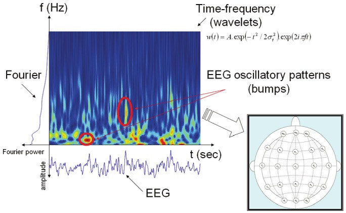
Possible representations of EEG brain dynamics. From the time-domain EEG signal, spectral information can be extracted, either in frequency or time-frequency domain. Afterwards, spatial maps are created (cf. plot at right hand side). However, such maps typically do not reveal the time-frequency structure (oscillatory patterns); we try to address this issue by developing audio representations.

Our viewpoint is rooted in computational intelligence. Artificial intelligence has many subfields, with varying purposes ranging from the classical “intelligent machine” projects (the Good Old-Fashioned Artificial Intelligence, GOFAI of Haugeland [1]) to the design of intelligent programs. Our approach belongs to the latter domain - and more specifically, a knowledge engineering approach (see e.g. [2]). Knowledge representation and knowledge engineering, when investigated at a sub-symbolic level, is generally referred to as computational intelligence, the most recent offshoot of artificial intelligence (see e.g. [3]). We advocate here a computational intelligence approach, based on the intelligent extraction of relevant information from EEG signals at a sub-symbolic level. In particular, the representation should be sparse and hence easy to parse; it should also represent relevant EEG features, such as amplitude, time-frequency content, and large-scale synchronization. In comparison, direct playback of the EEG (also termed as ‘audification’) would give an inaccurate and convoluted representation [4]. In summary, extracting meaningful information from EEG is the key point of our approach.

Furthermore, the audio representations should take the origin of the EEG signals into account, specifically, the brain areas the signals are recorded from (occipital, temporal, frontal, parietal, etc.). Those areas are not necessarily involved in the same functional processes, and need to be represented distinctively. We should be able to identify the contribution of each electrode.

At last, we should of course be able to interpret the audio representations (third condition). Therefore, a tractable representation is mandatory; the musical scores should be sufficiently sparse. Since EEG is typically recorded from multiple electrodes (e.g., 8, 16, 32, 64, 128, or 256 electrodes), it is essential to only represent the most salient features of the EEG as notes. Otherwise, too many notes will be played and the audio representation will be a cacophony.

So far, several methods for translating EEG into audio sequences have been proposed (see [7] for a review): spectral mapping sonification, distance mapping sonification [4], audio alarm for a surgical instrument [5], model based sonification for analysis of epileptic seizures [6], and discrete-frequency transform for brain computer interface [7]. To the best of our knowledge, however, none of those sonification approaches fulfill the three conditions for satisfactory representation of EEG.

In this paper, we develop an EEG sonification system that satisfies the three above conditions; we will refer to our system as “bump sonification (BUS)”, since it based on sparse time-frequency maps of EEG known as “bump models” [13] (Section 2).

As an illustration, we apply our EEG sonification system to a clinical problem (Section 3). We consider EEG signals from elderly patients suffering from mild cognitive impairment (MCI, a.k.a. predementia) and from age-matched control subjects [8]. All MCI patients in our EEG data set developed Alzheimer’s disease within a year and a half; the EEG signals were recorded in a ‘rest eyes-closed’ condition. We will use our BUS method as a diagnostic tool, where we try to distinguish MCI patients from agematched control subjects based upon the audio representation of the EEG. At last, we provide concluding remarks and ideas for future research (Section 4).

Bump sonification (BUS)

We explain here how we generate audio representations from EEG (see Figure 2). Our “bump sonification (BUS)” procedure consists of three steps: (1) preprocessing, including artifacts removal and dimensionality reduction based on Blind Source Separation (BSS) and/or Independent component analysis (ICA), (2) sparse time-frequency representation, (3) generation of music (“sonification”) from time-frequency maps (cf. Step 2).

Figure 2.

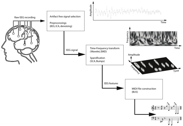
Bump sonification (BUS) system. First, sparse time-frequency (TF) maps are extracted from the EEG signals; those maps are then converted into music, stored as MIDI files. From top to bottom: EEG signal in time-domain, wavelet time-frequency representation, sparse time-frequency representation (a.k.a. “bump model”), and audio representation (music score). The EEG signal in this illustration is 2 sec long, and was sampled at a frequency of 1 kHz.

We describe the sparse time-frequency representation in Section 2.1. Next we discuss offline (Section 2.2) and online (Section 2.3) sonification.

Bump modeling

The time-frequency (TF) representation (see Figure 3, top) is obtained through the complex Morlet wavelet transform (Equation 1):

Figure 3.

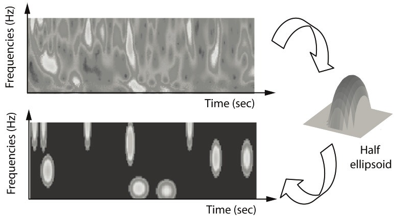
Example of bump modeling. The wavelet time-frequency (TF) map (top) is approximated by several parameterized functions (right), resulting in a sparse model (bottom) that captures the most prominent TF patterns.

where t is time, f is frequency, s_t is the time deviation, and A is a scalar normalization factor. This type of wavelet is well suited for time-frequency (TF) analysis of electrophysiological signals [9-11]), because of its symmetrical and smooth shape, both in time and frequency domains.

The resulting wavelet coefficients c_ft quantify the contribution of wave packets at time t with frequency f in the EEG signal. Wavelet coefficients c_ft are obtained for all T time steps and all F frequency steps.

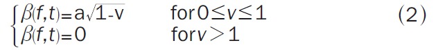
Next we sparsify the wavelet transform by means of bump modeling [12,13] (see Figure 3, bottom): we approximate a wavelet TF map by a set of elementary parameterized functions (“bumps”). Half ellipsoid functions were found to be the most suitable bump functions [13] (Equation 2):

where v= (e_f ² + e_t ²) with e_f = (f-μ_f) ∕ l_f and e_t = (t-μ_t) ∕ l_t. μ_f and μ_t are the coordinates of the center of the ellipsoid, l_f and l_t are the half-lengths of the principal axes, and a is the amplitude of the function.

A bump is fitted to the wavelet time-frequency map (within window W) by minimizing the cost function C (Equation 3):

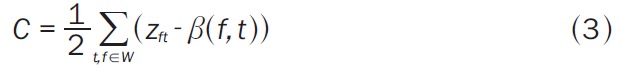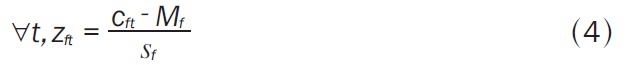
where the summation runs on all pixels within the window W, z_ft are properly normalized wavelet TF coefficients at time t and frequency f, and β(f,t) is the value of the bump function at time t and frequency f. In the present application, the TF coefficients c_ft where normalized with respect to the healthy control subjects as follows (Equation 4):

where M_f is the average of baseline activities μ_p^f at frequency f for all P control patients p (Equation 5):

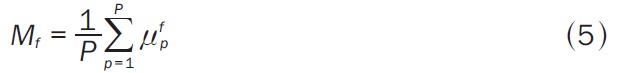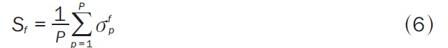
with μ_p^f = ‹1/T∑_t=1 ^T c_ft›p and S_f is the average of standard deviations σ_p^f at frequency f for all P control patients p (Equation 6):

with σ_p^f = ‹1/(T-1)∑_t-1 ^T(c_ft-μ_p^f)²›p. In this normalization scheme, large values represent activity that differs significantly from usual activity in healthy subjects; in other words, large z_ft values are associated with abnormal brain waves. Therefore, the normalized maps z_ft may help us, for instance, to detect brain disorders such as MCI and AD.

Bump modeling captures increased EEG activity in TF domain, compared to baseline EEG in healthy subjects. The corresponding wave packets (transient oscillations) are associated with transient local synchrony of neural assemblies [15].

Bump modeling was performed using the ButIF toolbox (Vialatte F, Sole-Casals J, Dauwels J, Maurice M, Cichocki A. Bump Time Frequency Toolbox software, version 1.0., 2008, freely available online at http://www.bps.brain.riken.jp/bumptoolbox/toolbox_home.html.), version 1.0.

Offline multi-channel sonification

EEG signals are often recorded from multiple channels. We translate multi-channel EEG signals into music scores according to the following principle (see Figure 4). Neighboring brain areas should be represented by similar notes, whereas remote brain areas should be represented by easily differentiable notes. Therefore, we determine the music notes from the following bump parameters: (1) Amplitude of the bump is converted into velocity of the note (valued between 40 and 127 in MIDI format), which indicates how loud the note is played. (2) Position of the electrode is encoded in the note pitch (C4 note = pitch 60 in MIDI format). We use a pentatonic scale (following progressions such as 60-63-65-67-70). Nearby electrodes are mapped to notes with similar pitch, and remote electrodes are mapped to notes with substantially different pitch. (3) Location and width of the bump in time is converted into onset and duration of the note (in ticks per square).

Figure 4.

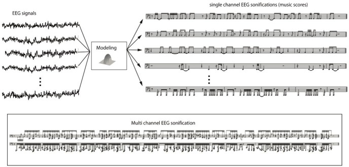
Multi-channel EEG sonification. In this example, 21-channel EEG is considered of length 20 sec and filtered between 5 and 25 Hz. The large amount of information is synthesized into a music score; this audio representation allows us to explore the signal dynamics and synchrony.

The resulting music score provides an alternative and useful representation of the EEG dynamics. However, there are two issues: (1) if the number of electrodes is large (more than 10), too many notes may be generated, potentially leading to cacophony; (2) if the frequency span is wide (e.g., 1-100Hz), the same problem may occur.

To avoid cacophony, we propose the following solutions: (1) if the number of electrodes is large, one may select the most representative electrodes. Alternatively, one may consider groups of electrodes, corresponding to certain brain areas (e.g., frontal and posterior areas). (2) if the frequency span is wide, one may divide it into frequency sub-bands.

We generate MIDI music by means of the Matlab MIDI Toolbox (Eerola T, Toiviainen P. MIDI Toolbox: MATLAB Tools for Music Research. University of Jyväskylä: Kopijyvä, Jyväskylä, Finland, 2004. Electronic version available from: http://www.jyu.fi/musica/miditoolbox/).

Online multi-channel sonification

So far we have considered offline sonification. Our bump sonification (BUS) procedure needs to be simplified for online use: Computing wavelet transforms and bump modeling is time-consuming, and would result in prohibitively large delays, which cannot be tolerated in real-time applications.

We propose the following fast sparsification procedure, as alternative to bump modeling, for real-time applications: (1) (offline) We select a set of frequency ranges, and determine corresponding thresholds (for z-score calculation, see below). (2) (Online) We smoothen the absolute value of the signal. In particular, we convolve the absolute value of the signal with a 4 cycles long Hanning window. Next we scale the smoothed curve by computing the z-score (cf. (3)), with pre-determined z-score parameters (cf. Step 1). A z-score value of zero corresponds to baseline, whereas a z-score of 1 corresponds to a value that is one standard deviation above baseline. We choose 1 as threshold value to generate music notes (see Step 3). (3) (Online) When the z-score crosses the threshold 1, we generate a music note. If the curve does not fall below threshold during 8 cycles, we generate a second music note. If the curve remains above threshold, we keep generating music notes every 4 cycles.

The z-score parameters are determined in a similar fashion as in the offline method (cf. Section 2.2, expressions (3)-(5)). The z-score parameters are now not computed for wavelet coefficients but for the smoothed signal instead.

The music notes are generated as follows: (1) The scaled smoothed curve (z-score) is converted into velocity of the note (valued between 40 and 127 in MIDI format), which indicates how loud the note is played. (2) Position of the electrode is encoded in the note pitch (C4 note = pitch 60 in MIDI format). We use a pentatonic scale (following progressions such as 60-63-65-67-70). Nearby electrodes are mapped to notes with similar pitch, and remote electrodes are mapped to notes with substantially different pitch. (3) When the scaled smoothed curve reaches threshold, a music note is triggered. While the curve remains above threshold, the note is played, for a maximum of 4 cycles; in other words, the duration of the note is determined by how long the curve remains above threshold. If the curve does not fall below threshold during more than 4 cycles, we keep generating music notes every 4 cycles.

This method generates music notes whenever the EEG activity is sufficiently strong over a sufficiently long period of time, as illustrated in Figure 5; this real-time approach is less precise than offline bump-based sonification (cf. Section 2.2), yet yields similar results.

Figure 5.

Two examples of real-time sparsification. The chosen frequency range is 6-8 Hz. (Top) Original EEG signal. (Second row) Band pass filtered EEG signal (6-8Hz). (Third row) Smoothed and z-score scaled activity in 6-8 Hz range; the signal is smoothed by convolving it with a 4 cycles long Hanning window (here: 571 msec). (Bottom row) The final sparse representation, used for real-time sonification.

Clinical application: diagnosis of MCI

The bump sonification (BUS) procedure has already been successfully applied to a brain computer interface application [16]. We will focus here on a clinical application: We will try to distinguish EEG from patients with mild cognitive impairment (MCI) and age-matched control subjects; specifically, we apply the BUS method to generate audio representations of the EEG signals, and try to discover significant differences between the audio representations from MCI patients and control subjects.

In the following, we will first describe our EEG data set (Section 2.4.1). Next we explain how we applied the BUS method to that data (Section 2.4.2). At last, we discuss how we evaluated the resulting music scores (Section 2.4.3).

EEG data

The EEG data used here have been analyzed in previous studies concerning early diagnosis of AD (see, e.g., [8,19,24]). Ag/AgCl electrodes (disks of diameter 8mm) were placed on 21 sites according to 10-20 international system, with the reference electrode on the right earlobe. EEG was recorded with Biotop 6R12 (NEC San-ei, Tokyo, Japan) at a sampling rate of 200Hz, with analog bandpass filtering in the frequency range 0.5-250Hz and online digital bandpass filtering between 4 and 30Hz, using a third-order Butterworth filter. We used a common reference for the data analysis (right earlobe), and did not consider other reference schemes (e.g., average or bipolar references).

The subjects comprise two study groups. The first consists of 25 patients who had complained of memory problems. These patients were diagnosed as suffering from mild cognitive impairment (MCI) when the EEG recordings were carried out. Later on, they all developed mild AD. The criteria for inclusion into the MCI group were a mini mental state exam (MMSE) score = 24, though the average score in the MCI group was 26 (SD of 1.8). The other group is a control set consisting of 56 age-matched, healthy subjects who had no memory or other cognitive impairments. The average MMSE of this control group is 28.5 (SD of 1.6). The ages of the two groups are 71.9 ± 10.2 and 71.7 ± 8.3, respectively.

All recording sessions were conducted with the subjects in an awake but resting state with eyes closed; the EEG technicians prevented the subjects from falling asleep (vigilance control). The length of the EEG recording is about 5 minutes, for each subject. After recording, the EEG data has been carefully inspected. Indeed, EEG recordings are prone to a variety of artifacts, for example due to electronic smog, head movements, and muscular activity. For each patient, an EEG expert selected by visual inspection one segment of 20s artifact free EEG, blinded from the results of the present study. Only those subjects were retained in the analysis whose EEG recordings contained at least 20s of artifact-free data. Based on this requirement, the number of subjects in the two groups described above was further reduced to 22 and 38, respectively. From each subject, one artifact-free EEG segment of 20s was analyzed (for each of the 21 channels).

Application of BUS method

We apply the offline BUS method (cf. Section 2.2) to all 60 subjects (22 MCI patients and 38 control subjects), resulting in one music score per subject (60 in total).

In this study, we analyze the EEG exclusively in the theta band (3.5-7.5 Hz). There are two reasons for this choice: Earlier studies of AD EEG (e.g., [17]) have reported strong effects in the theta range; moreover, this frequency band contains slow brainwaves, resulting in a relatively small number of music notes and hence a simple music score.

As in an earlier study [20], we wish to explore the interplay between frontal and parietal brain areas. Therefore, we only consider electrodes from those areas, i.e., F3, F3, Fz, P3, P4, and Pz. We aggregate the time-frequency bumps extracted from frontal areas in one group (group1 = F3, F3, Fz), and the bumps extracted from parietal areas in a second group (group2 = P3, P4, Pz). We associate low pitches (33, 35 and 37) to the frontal areas (group 1), and high pitches (57, 60 and 63) to the parietal areas (group 2), thereby following pentatonic scales.

Paradigm validation

We assess our sonification approach for MCI diagnosis by a purely quantitative analysis (statistical measures) and by a survey with human volunteers.

Statistical measures

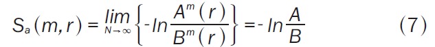
We consider the following statistical measures: sample entropy [19], number of notes, and a synchrony measure; we briefly review those measures here. The sample entropy is defined for a time series of N points. We first define the N-m+1 vectors X_m(i)={u(i+k):0≤k≤m-1}, as the vectors of m data points from u(i) to u(i+m-1). The distance between two such vectors is defined to be d[X_m(i),X_m(j)]=max_k{Іu(i+k)-u(j+k) І:0≤k≤m-1} the maximum difference of their corresponding scalar components. The sample entropy statistic is defined as (Equation 7):

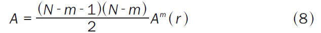
with (Equation 8)

and (Equation 9)

where N is the number of observations in the series. B^m(r) is the probability that two sequences match for m points (Equation 10):

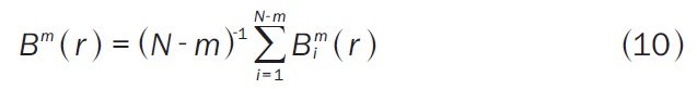where B_i^m(r) is (N-m-1)^-1 times the number of vectors X_m(j) within r of X_m(i). Similarly, A^m(r) is the probability that two sequences match for m+1 points (Equation 11):

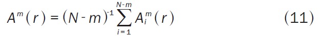where A_i^m(r) is (N-m-1)^-1 times the number of vectors X_m+1(j) within r of X_m+1(i). The scalar r is the tolerance for accepting matches. In our context, N is the total number of notes for the 6 electrodes. We set m=2 and r=1, and hence compute S_a(2,1). Therefore we looked upon organization along each different electrodes.

The number of notes is simply the overall number of notes for the six electrodes.

N₀ = N

The synchrony measure is defined as:

Sy = #V/N

where #V is the number of notes for which at least one note occurs at a neighboring electrode within 200msec; the latter is the maximum biologically plausible time window for synchronous activity.

Survey

Our BUS method is designed for human users instead of computer analysis. Therefore, a purely quantitative analysis (by means of statistical measures) is not sufficient to prove the effectiveness of our sonification method; we also validate it through a survey with human volunteers. Five volunteers are trained during 10 to 30 minutes to distinguish between audio sequences from MCI patients and control subjects (Samples available here: Vialatte F. MIDI multi channel EEG sonification of MCI and Control subjects, (Fronto-Parietal multichannel sonification). Riken BSI, april 2006. http://www.bsp.brain.riken.jp/~fvialatte/data/Iconip2006_midi/sample.htm). After the training period, the volunteers listen to a new database of 10 audio sequences (from 5 MCI patients and 5 control subjects). We ask the volunteers to score those new audio sequences (0: certainly MCI, 5: unsure, and 10: certainly healthy). We did not provide any further details about the new audio files.

Results

Our results for the statistical measures are summarized in Table 1. We applied the Mann-Whitney test to investigate whether the measures are statistically different in MCI patients in comparison to healthy control subjects. We observed statistically significant differences for all three measures; the best result is obtained for the synchrony measure Sy. Box plots of Sy are shown in Figure 6; from that figure, clear differences can be seen between MCI patients and control subjects: the synchrony is lower in MCI patients compared to healthy subjects.

Table 1.

Results for sample entropy (Sa), number of notes (No), and synchronization (Sy). Central columns list mean and standard deviation of the measures; right column lists the Mann-Whitney p-value (significant differences in medians when p < 0.01). Synchronization is the most discriminative feature (p-value marked in bold) between MCI patients and control subjects.

Feature	MCI	Control	Mann-Whitney p-value*
Sa(2, 1)	0.66±0.07	0.72±0.08	0.007
No	73.9±28	50.6±26	0.001
Sy (%)	3.52±1.04	5.10±1.96	4e10-4

^*The Mann-Whitney test is restricted to similarly shaped distributions. However, the standard deviation of Sy is substantially different in MCI patients compared to control subjects. Therefore, we log-normalize the Sy values before applying the Mann-Whitney test, in order to obtain more similar values of standard deviation in both subject populations.

Figure 6.

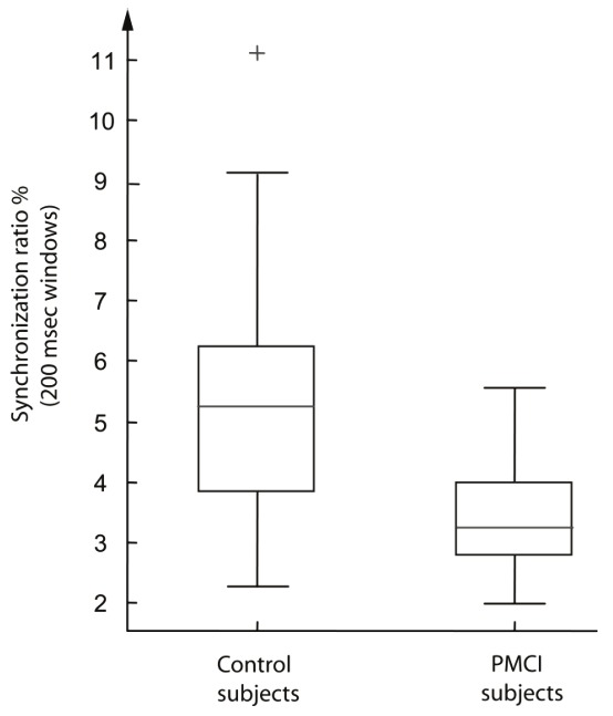
Synchrony index Sy (in percentage). The box plots suggest substantial differences in Sy between control subjects (left) and MCI patients (right).

As explained in the introduction, bump modeling is a simplified and sparse representation of EEG, which contains the most prominent components of the EEG in time-frequency domain. As we can see on Figure 7, significant differences can be observed for the bump concentration in the 6.5-7.5 Hz range. We investigate whether the information extracted by bump modeling is related to standard EEG statistics, in particular, relative Fourier power and coherence. Relative Fourier power is computed as the average over all 6 electrodes; likewise, coherence is computed as the average over all possible pairs of the 6 electrodes. We consider scatter plots of Sy vs. relative Fourier power and No vs. magnitude squared coherence (see Figure 8). From that figure, it can be seen that No does not seem to be correlated with Fourier power, and likewise Sy and coherence.

Figure 7.

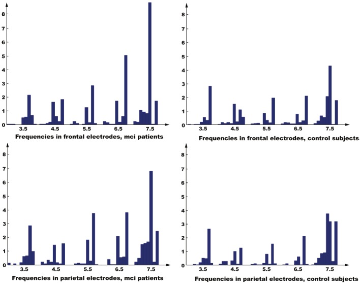
Histogram of bump frequencies f in the theta range (3.5-7.5 Hz), for frontal and parietal electrodes. (Left) MCI patients. (Right) Control subjects. The most significant difference between MCI patients and control subjects is observed in the 6-7.5 Hz range.

Figure 8.

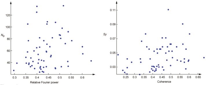
Sonification related measures vs. standard measures. Left: No vs. relative Fourier power (r=0.21, uncorrectedp=0.11); right: Sy vs. magnitude squared coherence (r=0.31, uncorrected p=0.02). The sonification relatedmeasures No and Sy do not seem to strongly correlate with the standard EEG measures (relative power and coherence).

The results for the survey are summarized in Figure 9. Remarkably, 4 out of 5 volunteers classified all music scores correctly. One of the volunteers made a few mistakes, resulting in an overall error of 11% (for all 5 volunteers). It is noteworthy that this result is for a subset of 10 subjects; the result for the entire data set (with 60 subjects) may be worse. Nevertheless, this experiment suggests that the music scores generated by the BUS procedure capture physiologically relevant features of the EEG. We now investigate this statement more rigorously. Concretely, we verify whether the scores of the volunteers (between 0 and 10) correlate with certain EEG statistics (see Figure 10). Such analysis should show us whether the volunteers perceived specific physiological aspects of the EEG, and as a result, were successful in labeling the music scores. Figure 10 shows that the subjects rating were strongly correlated with relative Fourier power and coherence. From this observation, we conclude that our sonification approach seems to adequately represent relevant aspects of the EEG.

Figure 9.

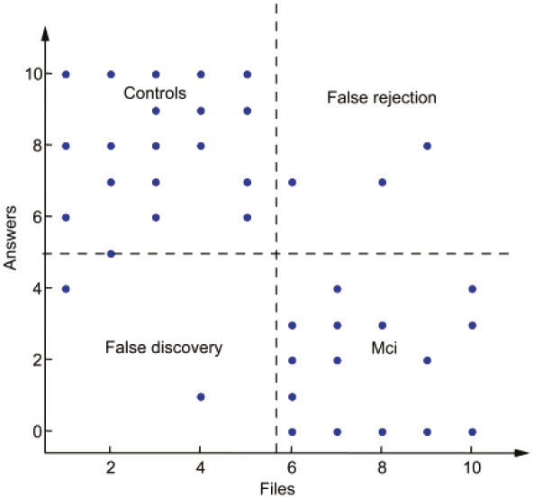
Result of the survey. Scores are shown for the new database of 10 audio sequences (5 control subjects and 5 MCI patients), for a total of 5 volunteers. Overall, 89% of the audio files were correctly classified. Interestingly, all the misclassifications stem from the same volunteer.

Figure 10.

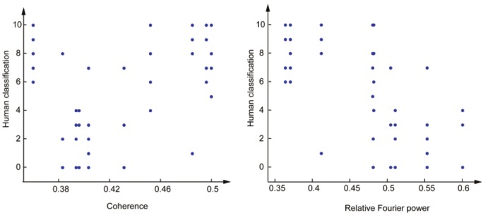
Scatterplot ofcoherence (left) and relativeFourier power (right)vs. survey score (0-10; cf.Section 3.3). Coherenceexhibits significant correlationwith the surveyscore (r=0.45, p=0.001),whereas Fourier relativepower and the surveyscore seem to bestrongly anti-correlated(r=-0.58, p=10^-5).

Discussion and conclusion

EEG signals evolve both in time and space, often resulting in highly complex patterns. Consequently, EEG is often either analyzed by simple tools (such as time-and space-averaging and Fourier power), which are often too rudimentary for neuroscience and clinical applications, see e.g. [22]), or by more complex methods, leading to results that are harder to visualize and interpret. For example, sparse bump models carry meaningful information about local and large-scale synchrony, which can for instance be quantified by stochastic event synchrony (SES) [20,21]. However, clinicians are typically hesitant to draw conclusions from statistical measures alone (e.g., SES parameters [20,21]); oftentimes, they prefer to follow their intuition and insights in the physiology of a patient at hand. In this paper, we developed an intuitive representation of multi-channel EEG data. In particular, we presented a physiologically inspired method for generating music scores from multi-channel EEG.

Audio representations of EEG may reveal oscillatory characteristics of the EEG that are less obvious from standard visual representations. Also, some clinicians and neuroscientists seem to find it easier to understand and memorize temporal patterns when presented as sound compared to visual representations [4]. Our method provides an intuitive audio representation of multi-channel EEG signals in time, frequency, and spatial domain; it may therefore prove to be well-suited for investigation of EEG dynamics, i.e., not only single-channel EEG characteristics (temporal and spectral), but also the interplay between EEG channels (e.g., long-distance synchronization activities [26]).

Our method was shown to be useful in a clinical application, where volunteers were asked to discriminate MCI patients from healthy subjects, based only on music scores extracted from their EEG. Interestingly, the volunteers were able to classify most of the music scores correctly; this result seems to suggest that the proposed sonification procedure retrieves reliable and physiologically relevant information from the EEG.

Moreover, our results for the MCI data are consistent with previous studies; loss of EEG synchrony in MCI and AD patients has been observed many times before (see [27] for a review), using a large variety of synchrony measures (e.g., coherence [23], mutual information [25] and synchronization likelihood [18,26]).

Besides clinical applications, one may also use real-time sonification in brain computer interfaces [17] and other applications in neuroengineering.

References

- 1.Haugeland J. Artificial Intelligence: The Very Idea. Cambridge, Mass: MIT Press; 1985. [Google Scholar]
- 2.Kasabov N. Evolving Connectionist Systems: The Knowledge Engineering Approach. London: Springer Verlag; 2007. [Google Scholar]
- 3.Engelbrecht AP. Computational Intelligence: An Introduction. 2nd edition. New York, USA: Wiley & Sons; 2007. [Google Scholar]
- 4.Hermann T, Meinicke P, Bekel H, Ritter H, Müller HM, Weiss S, editors. Sonifications for EEG data analysis; Proceedings of the 2002 International Conference on Auditory Display; July 2-5, 2002; Kyoto, Japan. pp. 37–41. [Google Scholar]
- 5.Jovanov E, Starcevic D, Karron D, Wegner K, Radivojevic V, editors. Acoustic Rendering as Support for Sustained Attention during Biomedical Procedures; International Conference on Auditory Display ICAD’98; 1998. [Google Scholar]
- 6.Baier G, Hermann T, editors. The sonification of rhythms in human electroencephalogram; Proceedings of ICAD 04-Tenth Meeting of the International Conference on Auditory Display; 2004; Sydney, Australia. [Google Scholar]
- 7.Miranda ER, Brouse A. Interfacing the Brain Directly with Musical Systems: On developing systems for making music with brain signals. Leonardo. 2005;38:331–336. [Google Scholar]
- 8.Musha T, Asada T, Yamashita F, Kinoshita T, Chen Z, Matsuda H, Masatake U, Shankle WR. A new EEG method for estimating cortical neuronal impairment that is sensitive to early stage Alzheimer’s disease. Clinical Neurophysiology. 2002;113:1052–1058. doi: 10.1016/s1388-2457(02)00128-1. [DOI] [PubMed] [Google Scholar]
- 9.Tallon-Baudry C, Bertrand O, Delpuech C, Pernier J. Stimulus specificity of phase-locked and non-phase-locked 40 Hz visual responses in human. Journal of Neuroscience. 1996;16:4240–4249. doi: 10.1523/JNEUROSCI.16-13-04240.1996. [DOI] [PMC free article] [PubMed] [Google Scholar]
- 10.Vialatte FB, Sole-Casals J, Cichocki A. EEG windowed statistical wavelet scoring for evaluation and discrimination of muscular artifacts. Physiol Measur. 2008;29:1435–1452. doi: 10.1088/0967-3334/29/12/007. [DOI] [PubMed] [Google Scholar]
- 11.Vialatte F, Bakardjian H, Prasad R, Cichocki A. EEG paroxysmal gamma waves during Bhramari Pranayama: a yoga breathing technique. Consciousness and Cognition. 2009;18:977–988. doi: 10.1016/j.concog.2008.01.004. [DOI] [PubMed] [Google Scholar]
- 12.Vialatte F. Modélisation en bosses pour l’analyse des motifs oscillatoires reproductibles dans l’activité de populations neuronales: applications à l’apprentissage olfactif chez l’animal et à la détection précoce de la maladie d’Alzheimer. Paris: Paris VI University; 2005. [Google Scholar]
- 13.Vialatte FB, Martin C, Dubois R, Haddad J, Quenet B, Gervais R, Dreyfus G. A machine learning approach to the analysis of time-frequency maps, and its application to neural dynamics. Neural networks. 2007;20:194–209. doi: 10.1016/j.neunet.2006.09.013. [DOI] [PubMed] [Google Scholar]
- 14.Press WH, Flannery BP, Teukolsky SA, Vetterling WT. Numerical Recipes in C: The Art of Scientific Computing. New York: Cambridge Univ. Press; 1992. pp. 425–430. [Google Scholar]
- 15.Vialatte FB, Dauwels J, Maurice M, Yamaguchi Y, Cichocki A. On the synchrony of steady state visual evoked potentials and oscillatory burst events. Cognitive Neurodynamics. 2009;3:251–261. doi: 10.1007/s11571-009-9082-4. [DOI] [PMC free article] [PubMed] [Google Scholar]
- 16.Rutkowski TM, Vialatte F, Cichocki A, Mandic DP, Barros AK, editors. Auditory Feedback for Brain Computer Interface Management - An EEG Data Sonifcation Approach. LNAI; KES2006 10th International Conference on Knowledge-Based & Intelligent Information & Engineering Systems; Bournemouth, England. 2006. pp. 1232–1239. [Google Scholar]
- 17.Vialatte F, Cichocki A, Dreyfus G, Musha T, Rutkowski T, Gervais R. Blind source separation and sparse bump modeling of time frequency representation of EEG signals: New tools for early detection of Alzheimer’s disease. IEEE Sign. Proc. Soc. Workshop on MLSP, Mystic, USA. 2005:27–32. [Google Scholar]
- 18.Babiloni C, Ferri R, Binetti G, Cassarino A, Forno GD, Ercolani M, Ferreri F, Frisoni GB, Lanuzza B, Miniussi C, Nobili F, Rodriguez G, Rundo F, Stam CJ, Musha T, Vecchio F, Rossini PM. Fronto-parietal coupling of brain rhythms in mild cognitive impairment: A multicentric EEG study. Brain Research Bulletin. 2006;69:63–73. doi: 10.1016/j.brainresbull.2005.10.013. [DOI] [PubMed] [Google Scholar]
- 19.Richaman JS, Moorman JR. Physiological time-series analysis using approximate entropy and sample entropy. Am J Physiol Heart Circ Physiol. 2000;278:2039–2049. doi: 10.1152/ajpheart.2000.278.6.H2039. [DOI] [PubMed] [Google Scholar]
- 20.Dauwels J, Vialatte F, Weber T, Cichocki A. Quantifying Statistical Interdependence by Message Passing on Graphs PART I: One-Dimensional Point Processes. Neural Computation. 2009;21:2152–2202. doi: 10.1162/neco.2009.04-08-746. [DOI] [PubMed] [Google Scholar]
- 21.Dauwels J, Vialatte F, Weber T, Musha T, Cichocki A. Quantifying Statistical Interdependence by Message Passing on Graphs PART II: Multi-Dimensional Point Processes. Neural Computation. 2009;21:2203–2268. doi: 10.1162/neco.2009.11-08-899. [DOI] [PubMed] [Google Scholar]
- 22.Scinto LFM, Daffner KR. Early diagnosis of Alzheimer’s Disease. Totowa, New Jersey, USA: Humana Press; 2000. [Google Scholar]
- 23.Adler G, Brassen S, Jajcevic A. EEG coherence in Alzheimer’s dementia. J Neural Transm. 2003;110:1051–1058. doi: 10.1007/s00702-003-0024-8. [DOI] [PubMed] [Google Scholar]
- 24.Brinkmeyer J, Grass-Kapanke B, Ihl R. EEG and the Test for the Early Detection of Dementia with Discrimination from Depression (TE4D): a validation study. Int J Geriatr Psychiatry. 2004;19:749–753. doi: 10.1002/gps.1162. [DOI] [PubMed] [Google Scholar]
- 25.Stam CJ, Montez T, Jones BF, Rombout SARB, van der Made Y, Pijnenburg YAL, Scheltens Ph. Disturbed fluctuations of resting state EEG synchronization in Alzheimer’s disease. Clinical Neurophysiology. 2005;116:708–715. doi: 10.1016/j.clinph.2004.09.022. [DOI] [PubMed] [Google Scholar]
- 26.Varela F, Lachaux JP, Rodriguez E, Martinerie J. The brainweb: phase synchronization and large-scale integration. Nature Reviews Neuroscience. 2001;2:229–239. doi: 10.1038/35067550. [DOI] [PubMed] [Google Scholar]
- 27.Dauwels J, Vialatte F, Cichocki A. Diagnosis of Alzheimer’s disease from EEG signals: where are we standing? Curr Alzheimer Res. 2010;7:487–505. doi: 10.2174/156720510792231720. [DOI] [PubMed] [Google Scholar]