Rigid Body Energy Minimization on Manifolds for Molecular Docking

Abstract

Virtually all docking methods include some local continuous minimization of an energy/scoring function in order to remove steric clashes and obtain more reliable energy values. In this paper, we describe an efficient rigid-body optimization algorithm that, compared to the most widely used algorithms, converges approximately an order of magnitude faster to conformations with equal or slightly lower energy. The space of rigid body transformations is a nonlinear manifold, namely, a space which locally resembles a Euclidean space. We use a canonical parametrization of the manifold, called the exponential parametrization, to map the Euclidean tangent space of the manifold onto the manifold itself. Thus, we locally transform the rigid body optimization to an optimization over a Euclidean space where basic optimization algorithms are applicable. Compared to commonly used methods, this formulation substantially reduces the dimension of the search space. As a result, it requires far fewer costly function and gradient evaluations and leads to a more efficient algorithm. We have selected the LBFGS quasi-Newton method for local optimization since it uses only gradient information to obtain second order information about the energy function and avoids the far more costly direct Hessian evaluations. Two applications, one in protein-protein docking, and the other in protein-small molecular interactions, as part of macromolecular docking protocols are presented. The code is available to the community under open source license, and with minimal effort can be incorporated into any molecular modeling package.

In this paper we describe a highly efficient minimization algorithm in the six dimensional (denoted as 6D) space of rigid affine transformations of macromolecules. This step is an integral component of many predictive docking algorithms. The challenge for predictive docking is to start with the coordinates of the unbound component molecules and to computationally obtain a model of the bound complex.^1–3 One of the component molecules, usually the larger, will be considered as the receptor, and the other the ligand. Our focus is restricted to protein receptors, and the ligand can be another protein, a drug-sized small molecule, or a molecular fragment. Assuming that the receptor is fixed at the origin of the coordinate system, the essential search space of docking consists of the 6D space of rotations and translations of the ligand. However, the search generally involves n additional variables that describe the conformational changes in one or both molecules, resulting in an extended search space that will be denoted as (6+n)D. The docking problem is defined as searching for the global minimum (or the lowest minima) of an energy/scoring function, denoted by E, in this space. A large variety of algorithms have been proposed in the literature to address this problem. In protein-protein docking, the essential 6D space can be searched using the Fast Fourier Transform (FFT) correlation approach^4–6 or by geometric matching.⁷ The sampling is usually followed by refinement, involving further minimization of the energy function E in both 6D and (6+n)D.³ The other frequently used method is Monte Carlo minimization, which combines random moves in 6D with minimizations in both 6D and (6+n)D.^8,9 There is a much larger variety of approaches to the docking of small molecules, including geometric matching, incremental construction from fragments of the ligand, and stochastic methods such as Monte Carlo and genetic algorithms.^10,11

Independently of the algorithm used for sampling the conformational space, virtually all docking algorithms also include some type of local continuous minimization of the energy function E in order to remove steric clashes and obtain more reliable energy values.³ The minimization algorithm we propose in this paper addresses this problem. The commonly used algorithms for this purpose either define the problem as an all-atom optimization where the rigidity is indirectly imposed by interatomic forces, or they include rigidity constraints by adding them to the objective function of optimization via Lagrange multipliers. In both cases the domain of the optimization is a high dimensional space. By contrast, we define the optimization on the 6D manifold (i.e., a space which locally resembles a Euclidean space) of rigid affine transformations of the ligand. A rigid transformation can be represented by a pair of rotation and translation (R,t). Here the rotation R is represented by a 3 ×3 orientation-preserving matrix, an element of the so-called Special Orthogonal group SO(3), and t is a 3-dimensional translation vector, i.e., t ∈ ℜ³. The rigid body transformations can be considered as SO(3) ×ℜ³, the direct product of SO(3) and ℜ³. We note that the problem of parameterizing the group of rotations has been of interest since Euler’s related work in 1776 and has received significant attention in the robotics area^12–14 but less so in modeling biomolecular conformations.¹⁵ For instance, it is known that there exists no global parametrization without singular points for this space. However, we can locally map the manifold onto a subset of the Euclidean space, and thereby redefine the optimization as a problem over a Euclidean space. We use a local parametrization using the so called exponential coordinates. In this parametrization, the tangent space of the manifold at any point, a Euclidean space, is locally mapped onto the nonlinear manifold. A simple example of a manifold and its natural exponential map, is a circle, S¹. Globally, S¹ is a curved space; however, locally, each piece of a circle is similar to a part of a line. More specifically, consider a tangent line to a circle at any point and let φ denote the coordinate of a point on this line. Then, we have a natural mapping of this line onto the circle in the complex plane by exponentiating φ → exp^iφ. This transformation can be generalized to any manifold. More details for the manifold of rigid body transformations are given in the paper.

Given the exponential coordinates, the rigid body energy minimization is defined on the 6-dimensional Euclidean space ℜ⁶, and any traditional minimization method can be used. We have selected the LBFGS¹⁶ quasi-Newton method since it uses only gradient information to obtain second order information about the energy function, and avoids the far more costly direct Hessian evaluations. The advantage of this manifold optimization formulation is that it searches over a significantly lower-dimensional space, leads to a much smaller number of costly function and gradient evaluations, and results in a significantly more efficient optimization algorithm.

We describe applications of the new algorithm to both protein-protein and protein-fragment docking. The first application complements our docking program PIPER,⁶ also implemented in the heavily used docking server ClusPro.¹⁷ PIPER performs exhaustive evaluation of an energy function in discretized 6D space of mutual orientations of two proteins using the fast Fourier transform (FFT) correlation approach. We sample 70,000 rotations, which approximately correspond to sampling at every 5 degrees in the space of Euler angles. In the translational space, the sampling is defined by the 1.2 Å grid cell size. PIPER is used with a “smooth” scoring function, including terms representing shape complementarity, electrostatic, and desolvation terms, the latter represented by the pairwise interaction potential DARS (Decoys As the Reference State).¹⁸ We call the potential “smooth” because the repulsive contributions in the shape complementarity terms are selected to allow for a certain amount of overlaps. While this helps to retain more near-native docked conformations, it also implies that the structures generated by PIPER are generally not free of steric clashes. To remove steric clashes, the current version of ClusPro minimizes the CHARMM¹⁹ energies of the docked structures generated by PIPER. As will be shown, this step can be made much more efficient by the application of the novel method described in this paper.

The second application to protein-small molecule docking complements our protein mapping program FTMap,²⁰ also implemented as a server. Mapping places molecular probes—small organic molecules that vary in size and shape—on a dense grid around the protein to identify potentially favorable binding positions. The method is based on X-ray and NMR screening studies showing that the binding sites of proteins also bind a large variety of fragment-sized molecules. Similarly to PIPER, for each probe type the first step of FTMap is global sampling of the 6D space using the FFT correlation approach. In the current version of FTMap the docked structures generated by this calculation are minimized off-grid using the CHARMM potential, primarily for removing steric clashes and obtaining better energies, since only a few of the lower-energy probe clusters are retained for further processing. As in protein-protein docking, the traditional all-atom CHARMM minimization is computationally expensive, and thus replacing it with our novel method provides substantial benefits.

1 Methods

We assume the larger protein, the receptor, is fixed at the origin of the coordinate system. A rigid body motion/transformation of the ligand is specified by a pair of translation and rotation motions, (R,t). This rigid body motion corresponds to a receptor-ligand conformation with its associated energy. The space of all rigid body motions constitutes a 6D nonlinear manifold and the optimization problem we consider is a minimization of conformational energy over this nonlinear manifold.

1.1 Formulation of rigid body optimization

A rigid body transformation can be represented by a rotation R and a translation t, i.e., (R,t). The rotation R is represented by a 3 ×3 orientation-preserving matrix, i.e., an element of the so-called Special Orthogonal group,

$$SO(3)=\{R\in {\mathfrak{\Re }}^{3\times 3};R^{T}R=I;\mathit{det}(R)=1\},$$

and t is a 3 dimensional translation vector t ∈ ℜ³.

We note that there is not a unique way to associate (R,t) with a rigid body motion. The unspecified element is the center of rotation. In our formulation, we select an initial center of rotation p in ℜ³. For example, this point may be the center of mass of the ligand, the center of mass of the interface between the ligand and the receptor, or any point on the line connecting the center of mass of the ligand and the center of mass of the receptor. Given this choice, the rigid body transformation we associate with (R,t) transforms a point q in ℜ³ as follows.

$$q\to R(q-p)+p+t.$$

In this transformation, atoms of the ligand are rotated around p by an amount specified by the rotation matrix R and are translated by an amount equal to t.

1.2 Local parametrization of SO(3) ×ℜ³ via the exponential map

As mentioned earlier, we use a local parametrization approach via exponential coordinate parameters. In this parametrization, the tangent space to the manifold, which is a Euclidean space, is mapped to the nonlinear manifold using an exponential map. The geodesics of the tangent space, namely straight lines, are mapped to the geodesics of the manifold. For this reason, the exponential map parametrization is a particularly suitable local parametrization.

1.2.1 The exponential map coordinates

ℜ³ is a Euclidean and linear manifold and its standard coordinates provide a global parametrization. We define the local parametrization SO(3) manifold via the exponential map below. Parametrization for SO(3) × ℜ³ is simply the product of parameterizations for SO(3) and ℜ³.

The tangent space of SO(3) at I, the identity of the group of rotations, is denoted by so(3) and can be identified with the space of 3 ×3 skew-symmetric matrices. For ω = (ω₁, ω₂, ω₃)^T ∈ ℜ³, let

$$[\omega ]=\left[\begin{array}{ccc}0& -{\omega }_3& {\omega }_2\\ {\omega }_3& 0& -{\omega }_1\\ -{\omega }_2& {\omega }_1& 0\end{array}\right].$$

The exponential map at identity I ∈ SO(3) maps the tangent space at identity, so(3), to SO(3). It is defined by

$${exp}_I(\omega )=e^{[\omega ]},$$

where the expression on the right hand side of the equation is a matrix exponential. The right hand side simplifies to give what is known as the Rodrigues formula

$$e^{[\omega ]}=I+\frac{sin(|\left|\omega \right||)}{\left|\right|\omega \left|\right|}[\omega ]+\frac{(1-cos(\left|\right|\omega \left|\right|))}{{\left|\right|\omega \left|\right|}^2}{[\omega ]}^2,$$

where ||ω|| is the Euclidean norm of ω.

The exponential map defined on the tangent space at R ∈ SO(3) is simply defined as exp_R(ω) = Re^[ω]. Geodesics of SO(3) are given by R(u) = R₀e^[ω]u, ω ∈ ℜ³ and u ∈ R and correspond to the projection by the exponential map of lines going through the origin on the tangent space.

The exponential map of SO(3) × ℜ³ can be easily obtained from that of SO(3). Consider the exponential map at the identify of the product group SO(3) × ℜ³, i.e., (I,0). The tangent space can be identified with ℜ⁶. Let (ω, υ) ∈ ℜ⁶ be a point of the tangent space. Then,

$${exp}_{(I,\mathbf{0})}(\omega ,\upsilon )=(e^{[\omega ]},\upsilon ).$$

Therefore,

$${exp}_{(I,\mathbf{0})}:{\mathfrak{\Re }}^6\to SO(3)\times {\mathfrak{\Re }}^3$$

defines a local parametrization for SO(3) × ℜ³ in the neighborhood of (I, 0).

1.3 The optimization algorithm

Given the exponential map parametrization, the rigid body energy minimization is defined on the 6-dimensional Euclidean space ℜ⁶. From among the many deterministic algorithms available to solve local minimization problems on a Euclidean space, we have selected the quasi-Newton method of Limited memory BFGS (LBFGS).¹⁶ In our parametrization, the gradient and the Hessian of the energy function with respect to the parameters of optimization can be explicitly calculated. However, these are costly operations, evaluating the Hessian being significantly more costly than evaluating the gradient. Our choice of LBFGS has been based on the fact that it uses only gradient information to obtain second order information about the energy function.

1.3.1 Gradient of the Energy Function With Respect to Exponential Map Parametrization

Let q = (q₁, ···, q_ml) be the initial position of the ligand where m_l is the number of ligand atoms and every element of q indicates the position of a ligand atom. Let also p, a fixed point in ℜ³, represent the initial center of rotation. Furthermore, consider the exponential coordinate parametrization of SO(3) × ℜ³ described above and let (ω, υ) ∈ ℜ⁶ be a point in the tangent space of SO(3) × ℜ³ at (I, 0). ω represents the rotation parameters and υ, the translation parameters. Then, the energy function can be views as a function of (ω, υ). More specifically,

$$E[(\omega ,\upsilon )]=E[exp([\omega ])(q_1-p)+p+\upsilon ,\cdots ,exp([\omega ])(q_{m_l}-p)+p+\upsilon ].$$

The only components of gradient evaluation that require some discussion are the terms ∂ exp([ω])/∂ω_i.

Using the Rodrigues formula, we have

$$\frac{\partial exp([\omega ])}{\partial {\omega }_i}=\frac{\partial }{\partial {\omega }_i}\left(\frac{sin(|\left|\omega \right||)}{\left|\right|\omega \left|\right|}[\omega ]+\frac{(1-cos(\left|\right|\omega \left|\right|)}{{\left|\right|\omega \left|\right|}^2}{[\omega ]}^2\right).$$

For ||ω|| near zero, we make the following approximations. $\frac{sin(|\left|\omega \right||)}{\left|\right|\omega \left|\right|}\simeq 1-\frac{{\left|\right|\omega \left|\right|}^2}{3!}$ and $\frac{1-cos\left|\right|\omega \left|\right|}{{\left|\right|\omega \left|\right|}^2}\simeq \frac{1}{2}-\frac{{\left|\right|\omega \left|\right|}^2}{4!}$.

1.3.2 Limited memory BFGS (LBFGS)

We denote points in ℜ⁶ by x. The LBFGS method consists of the following iterations¹⁶

$$x_{k+1}=x_k+{\alpha }_k{d}_k,$$ (1)

where

$$d_k=-H_k\nabla E_k,$$ (2)

and where ∇E_k is the gradient of the energy function, H_k is the LBFGS approximation of the inverse of the Hessian of the energy function, and α_k is an appropriately selected step-length satisfying the so-called Wolf conditions.¹⁶

As pointed out in,¹⁶ the choice of H₀ influences the behavior of the algorithm. When the diagonal entries of the Hessian are all positive, it is recommended to let H₀ be a diagonal matrix with the diagonal entries of the inverse of the Hessian. Given that in our problem the diagonal entries of the Hessian are sometimes negative, we use the identity matrix as the initial H₀. We use the line search algorithm described in the literature.²¹

To avoid moving away from a local minimum that is in the vicinity of the initial configuration, we avoid big rotational moves in the iterations of the algorithm. In the initial configuration there may be clashes between the ligand and the receptor, and the energy and its gradient may be very large. As a result, it is possible that at the first step the algorithm may suggest a big rotational move. In such cases, we scale the diagonal elements of the initial Hessian approximation corresponding to the rotational parameters to avoid big rotational moves. At subsequent steps, if the algorithm suggests making a big rotational move, we re-initialize the Hessian to the identity matrix and restart LBFGS.

Figure 1 (a) & (b) provide a schematic representation of our parametrization approach. The local optimization is performed on the tangent space. Figure 1(a) shows the evolution of the optimization algorithm on the tangent space until a local minimum is reached. The solution is then mapped to the manifold of rigid body transformations. Figure 1(b) shows the evolution of the optimization algorithm in terms of the movement of the ligand. The ligand is shown by a small sphere with an attached coordinate frame that shows its orientation. Translational moves can be seen by the movement of the center of the sphere and rotational moves by the rotation of the coordinate frame.

Figure 1.

(a) The sphere represents the SO(3)×ℜ³ manifold and the plane represents the tangent space at the identity. The dots on the tangent space correspond to optimization steps and the position of each dot corresponds to the first two coordinates of the exponential map parametrization at the identity. The position produced by the local optimization algorithm on the tangent space after every ten steps is shown by a color dot. Colors correspond to the energy value at that step of the optimization. Red represents high energy and blue represents low energy. Each step of the optimization is connected by a line to the next step. (b) Each sphere represents the center of mass of the ligand at every ten step of the optimization of the 1AY7 complex. The color codes are the same as in (a). The axes connected to each sphere show the rotational axes of the ligand at that step of the optimization.

Figures 2 presents the configuration of the receptor and ligand for the complex 1AY7 before and after the application of the local minimization.

Figure 2.

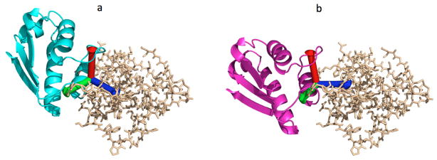
a) 1AY7 complex before rigid body minimization; the coordinate axes is centered at the center of rotation. b) 1AY7 complex after rigid body minimization; the axes rotate and translate with the ligand and settle at a new position.

2 RESULTS AND DISCUSSION

In this section we describe the experimental setup and results from the application of the proposed manifold optimization algorithm to protein-protein docking and protein-small molecule docking. We compare the performance of the manifold optimization algorithm with the optimization algorithms currently being used. Our comparison is based on the quality of solutions generated and the computational efficiency of the algorithms. The results show that the quality of solutions produced by the manifold optimization algorithm is equal or slightly better than the alternatives tested but its computational efficiency is significantly superior to them.

2.1 Application to protein-protein docking

As mentioned in the introduction, the first application of the new method is to the off-grid minimization of structures generated by the PIPER docking program.⁶ Currently, the rigid body minimization option of the CHARMM package is used for this purpose. Therefore, we compare the proposed manifold optimization with the rigid body minimization option of the CHARMM package.

The results reported here are based on the application of the two algorithms to 9 enzyme-inhibitor, 6 antigen-antibody, and 4 other complexes selected from the protein docking benchmark set.²² In each case, the unbound structures of the component proteins of the complex were downloaded from the Protein Data Bank.²³ These structures were docked using PIPER. Then, for each protein pair, the 1500 lowest energy structures were refined by minimizing their CHARMM energy using the rigid body minimization option of the CHARMM and the proposed manifold optimization algorithm. This test set was selected in order to provide a diverse and representative set of complexes, and for each complex, a large set of initial conditions for comparing the optimization algorithms. While we selected only 19 protein-protein complexes, for each complex the minimizations were started from 1500 different conformations. Thus, the two algorithms are compared based on about 28,000 test cases.

As discussed earlier, in our algorithm we have the flexibility of selecting a center of rotation for rigid body transformation. We examined two different centers of rotation: (i) the center of mass of the ligand and (ii) the center of mass of the contact residue interfaces of the ligand. The contact residue interface of the ligand is defined as the residues of the ligand which have at least one atom within 10 Å of an atom of the receptor. Our experiments showed that option (ii) produced better results. These results are reported in what follows.

We compare the two algorithms based on the quality of solutions they generate and their computational efficiency. To assess the quality of the solutions, we consider the ensemble of 1500 solutions produced for each protein pair. The solutions where the local minima found by the two algorithms are within 0.01 Å RMSD distance of each other, or when the difference between the energies of the solutions found are less than $0.01\frac{\mathit{kcal}}{\mathit{mol}}$ are considered as ties. If the local minimum found by one of the algorithms is further than 10 Å from the initial conformation, the solution is considered as a failure, as we expect to find some local minimum within a 10 Å RMSD range of the initial conformation. The cases where both algorithms fail and there is no basis for comparison are removed from those reported. In all other cases, the quality of the solution of one algorithm relative to the other is considered as superior if it has a lower energy (by more than $0.01\frac{\mathit{kcal}}{\mathit{mol}}$). For each complex, the number of cases where one algorithm was found to be superior to the other as well as the number of ties are reported in Table 1.

Table 1. Comparison of the quality of solutions & computational efficiency of manifold optimization (MO) with CHARMM rigid body minimization (CH).

Each complex is identified by its 4-letter PDB²³ code in the first column of the table. The second column identifies the type of the complex (E: Enzyme-inhibitor, A: Antigen-antibody, and O: Other). The third column lists the number of conformations in which CHARMM (denoted by CH) converged to a local minimum with lower energy than one produced by the manifold optimization algorithm (denoted by MO) and therefore had a better performance than MO. The fourth column presents the number of cases in which the manifold optimization algorithm was superior to CHARMM, and the fifth column reports the number of cases where the two algorithms performed similarly. The sixth column lists the average number of energy function evaluations in CHARMM and, finally, the last column reports the average number of energy function evaluations of the manifold optimization algorithm. The last row of the table reports average results over all the complexes tested.

Complex description		Quality of solutions: Which performs better			Computational efficiency: Average no. of steps
Complex	Type	CH > MO	MO > CH	MO = CH	CH	MO
1AVX	E	95	240	890	1027	111
1AY7	E	259	267	374	1650	116
1EAW	E	177	276	900	578	93
1MAH	E	316	319	364	869	134
1PPE	E	202	246	1044	453	125
1R0R	E	154	284	1020	638	113
2PCC	E	328	377	472	990	143
2SIC	E	351	164	479	754	104
2SNI	E	281	222	696	599	110
1FSK	A	173	475	814	1145	110
1NCA	A	85	182	875	1726	121
1WEJ	A	344	443	630	820	125
2JEL	A	432	328	507	946	120
1E6J	A	228	260	893	606	102
1AHW	A	188	595	489	1285	105
1B6C	O	165	838	230	305	102
1BUH	O	179	688	503	209	117
1GLA	O	114	880	276	227	98
1GPW	O	90	954	252	1094	101
		17.4%	33.6%	49.0%	7.4	1

As a measure of computational efficiency of each algorithm, we have selected the number of energy function evaluations needed to converge to a local minimum. Given that energy function evaluations are the most costly operations, their number justifiably characterizes the run time efficiency of the algorithm. Furthermore, since the same energy function is used for both algorithms, the number of energy function evaluations is a fair comparison between the runtime of the two algorithms.

Results From both algorithms, with center of rotation being the center of mass of the contact residue interface, is reported in Table 1. Based on these results it can be seen that our proposed algorithms leads to a a better performance and, more importantly, is on average about 7.4 times faster than CHARMM.

2.2 Application to Protein Mapping

Our second application of the manifold optimization algorithm is to protein-small molecule docking to be used as a complement to our protein mapping program FTMap.²⁰ Mapping places molecular probes–small organic molecules that vary in size and shape–on a dense grid around the protein to identify potentially favorable binding positions. Similarly to PIPER, for each probe type the first step of FTMap is global sampling of the 6D space using the FFT correlation approach. In the current version, the docked structures generated by this calculation are minimized off-grid using the CHARMM potential and an all-atom minimization. We therefore compare the proposed manifold optimization with this all atom minimization. To compare the two algorithms 14 protein structures, shown in Table 2, were selected from the Protein Data Bank.²³ Seven of these proteins have been the subject of a recent mapping study.²⁴ All ligand and bound water molecules are removed prior to mapping. 16 small organic molecules (ethanol, isopropanol, isobutanol, acetone, acetaldehyde, dimethyl ether, cyclohexane, ethane, acetonitrile, urea, methylamine, phenol, benzaldehyde, benzene, acetamide and ndimethylformamide) are used as probes. For each target, FTMap performs a grid search using the Fast Fourier Transform (FFT) correlation approach in order to find the low energy docked positions of the probes. Each complex is evaluated using an energy expression that includes van der Waals and electrostatic interaction energy terms as well as solvation effects.²⁰ In the current version of FTMap, the 2000 most favorable docked positions of each probe are then energy-minimized using the CHARMM force field and all-atom minimization. During this minimization the probe molecules are considered fully flexible, but the atoms of the receptor protein are taken as fixed.

Table 2. Comparison of the quality of solutions & computational efficiency of manifold optimization (MO) against all-atom minimization (FA) for all probes and rigid only subset.

Complexes are identified by their 4-letter PDB²³ code in the first column of the tables. Columns two to six correspond to full probe set. Columns seven to eleven correspond to rigid only subset. The second column lists the number of conformations in which all-atom minimization (denoted by FA) converged to a local minimum with lower energy and performed better than manifold optimization. The third column presents the number of cases in which manifold optimization produced a better result. The forth column reports the number of ties between the two algorithms. The fifth column lists the average number of energy function evaluations by all-atom minimization. The sixth column corresponds to the average number of energy function evaluations by the manifold optimization algorithm. The seventh column lists the number of conformations in which all-atom minimization (denoted by FA) converged to a local minimum with lower energy and performed better than manifold optimization. The eights column presents the number of cases in which manifold optimization produced a better result. The ninth column reports the number of ties between the two algorithms. The tenth column lists the average number of energy function evaluations by all-atom minimization, and, finally, the last column corresponds to the average number of energy function evaluations by the manifold optimization algorithm.

	All probes					Subset of rigid only probes
	Quality of solutions: Which performs better			Efficiency: no. of steps		Quality of solutions: Which performs better			Efficiency: no. of steps
Protein	FA > MO	MO > FA	MO = FA	FA	MO	FA > MO	MO > FA	MO = FA	FA	MO
2CAB	6094	7144	17538	406	58	2473	4662	14366	388	58
1IVG	6952	5994	17014	382	57	2430	3675	14531	366	55
1BBC	6910	8159	14916	414	63	2790	5520	12715	398	63
1F5L	6871	6176	17170	397	58	2590	4003	14264	381	58
1S3E	5559	4876	16897	394	55	1922	3514	14035	382	55
2B23	5687	4278	19919	369	34	1720	2743	16497	350	33
2O8T	7240	5935	17261	391	58	2441	4033	14789	375	57
1W50	6925	4926	19044	373	37	2117	3036	16130	355	36
1HCL	5633	5998	16531	387	39	1974	3995	13664	371	38
1JEE	4891	3267	15783	351	36	1285	2102	13484	337	35
1YES	5564	7306	17556	394	42	2339	4704	14310	377	42
1PUD	6411	5451	19229	381	40	2270	3291	15930	363	38
1THS	6164	5242	17718	378	39	2192	3470	14631	362	38
1BN5	6312	5498	18552	376	38	2072	3626	15488	359	38
	21.1%	19.4%	59.5%	8.3	1	10.6%	18.2%	71.2%	8.0	1

Similarly to the protein docking case we compare the two off-grid minimization algorithms based on the quality of their solutions and their computational efficiency. The cases where the local minima found by the two algorithms are within 0.05 Å RMSD distance of each other, or their energy differences are less than $0.01\frac{\mathit{kcal}}{\mathit{mol}}$, are considered ties. In the manifold optimization algorithm, selecting the center of rotation as the center of mass of the ligand produced better results and these are the results we report.

One of the basic advantages of mapping relative to docking is that due to the use of rigid small molecules as probes we can perform an exhaustive sampling of the protein surface. In fact, 11 of the 16 probes used by FTMap have no rotatable bonds, whereas the other five have a single rotatable C-O bond, allowing for the rotation of the H atom of an OH group. Given that the manifold optimization algorithm does not take the flexibility of the rotatable OH bond into account, we expect the all-atom optimization algorithm to have a somewhat better overall performance in terms of the energy values if all 16 probes are considered. To give an indication of the impact caused by not accounting for the rotatable bonds, we report two comparisons of the optimization algorithms, the first based on including all probes, the second based on considering only rigid probes.

The comparison results based on all probes, and rigid only probes are presented in Table 2. As can be seen, when all probes are included, the quality of the solutions produced by all-atom minimization is slightly better than that of manifold optimization algorithm, while the manifold optimization algorithm is approximately 8 times faster than the all-atom minimization algorithm. When we restrict ourselves to rigid probes the rigid body algorithms is not only faster, but also provides lower energies. As noted, most probes used for mapping are rigid. If necessary, the presence of one rotatable bond in a probe can be taken into account by using several conformers, and selecting the lowest energy. Since the rigid body minimization is more than eight times faster than the all-atom one, with a few rotamers the algorithm still remains competitive.

Next, we provide another comparison between the two optimization algorithms based on the hot spots they identify. The goal of FTMAP²⁰ is to find the hot spot on the receptor, namely the positions which attract the probes after minimization. To compare the two algorithms based on this criterion we discretize the space by considering a grid of cell size 0.8 Å. We assign each atom of a probe after minimization to a grid point that is closest to it and compute the total number of atoms assigned to each grid point by each algorithm. This leads to two grid-size vectors of integers.

We consider two different measures to evaluate the similarity of these two vectors that reflect on the similarity of hot spots identified by the two algorithms. We calculate the norm of the difference of these two vectors and normalize it by dividing by the norm of the vector produced by all-atom minimization. The second measure is the correlation between the two vectors. The results are presented in Table 3 and Table 4. Table 3 provides the results based on the probes while Table 3 presents the results based on the proteins considered.

Table 3.

Comparison of the density of solutions of manifold optimization (MO) with all-atom optimization (FA). The results are shown for each probe.

Probe	Normalized distance	Correlation
acetamide	0.10	0.994
acetone	0.07	0.997
acetonitrile	0.06	0.997
acetaldehyde	0.09	0.995
methylamine	0.08	0.996
benzene	0.10	0.994
cyclohexane	0.05	0.998
ndimethylformamide	0.09	0.995
dimethyl ether	0.06	0.997
ethane	0.03	0.999
urea	0.21	0.978

Table 4.

Comparison of the density of solutions of manifold optimization (MO) with all-atom optimization (FA). The results are shown for the proteins considered.

Protein	Normalized distance	Correlation
2CAB	0.07	0.997
1IVG	0.03	0.999
1BBC	0.02	0.999
1F5L	0.03	0.999
1S3E	0.06	0.998
2B23	0.02	0.999
2O8T	0.03	0.999
1W50	0.02	0.999
1HCL	0.09	0.995
1J2E	0.03	0.999
1YES	0.07	0.997
1PUD	0.03	0.999
1THS	0.05	0.999
1BN5	0.04	0.998

In both cases the results indicate that the performance of the two algorithms, in terms of identifying hot spots, are very similar.

3 Conclusions

In this paper, we introduce a new algorithm for rigid body local minimization of macromolecules. We note that the natural space of rigid body transformations is a nonlinear 6-dimensional manifold. We use a canonical parametrization of this manifold via the exponential map. This parametrization allows us to define the local optimization as an optimization on a 6-dimensional Euclidean space, namely, on a space of far lower dimension when compared with commonly used alternatives. As a result, the optimization requires far fewer costly function and gradient evaluations and leads to a more efficient algorithm. We have selected the LBFGS quasi-Newton method for local optimization since it uses only gradient information to obtain second order information about the energy function and avoids the far more costly direct Hessian evaluations. Two applications, one in protein-protein docking, and the other in protein-small molecular interactions, as part of macromolecular docking protocols are presented. Our experimental results show about an order of magnitude improvement in computational efficiency when compared with alternatives. The code is available to the community under open source license, and with minimal effort can be incorporated into any molecular modeling package.

References

- 1.Halperin I, Ma B, Wolfson H, Nussinov R. Proteins. 2002;47:409–443. doi: 10.1002/prot.10115. [DOI] [PubMed] [Google Scholar]
- 2.Smith G, Sternberg M. Curr Opin Struct Biol. 2002;12:28–35. doi: 10.1016/s0959-440x(02)00285-3. [DOI] [PubMed] [Google Scholar]
- 3.Vajda S, Kozakov D. Curr Opin Struct Biol. 2009;19:164–170. doi: 10.1016/j.sbi.2009.02.008. [DOI] [PMC free article] [PubMed] [Google Scholar]
- 4.Katchalski-Katzir E, Shariv I, Eisenstein M, Friesem A, Aflalo C, Vakser I. Proc Natl Acad Sci USA. 1992;89:2195–2199. doi: 10.1073/pnas.89.6.2195. [DOI] [PMC free article] [PubMed] [Google Scholar]
- 5.Chen R, Li L, Weng Z. Proteins. 2003;52:80–87. doi: 10.1002/prot.10389. [DOI] [PubMed] [Google Scholar]
- 6.Kozakov D, Brenke R, Comeau SR, Vajda S. Proteins. 2006;65:392–406. doi: 10.1002/prot.21117. [DOI] [PubMed] [Google Scholar]
- 7.Schneidman-Duhovny D, Inbar Y, Polak V, Shatsky M, Halperin I, Benyamini H, Barzilai A, Dror O, Haspel N, Nussinov R, Wolfson HJ. Proteins. 2003;52:107–112. doi: 10.1002/prot.10397. [DOI] [PubMed] [Google Scholar]
- 8.Fernandez-Recio J, Totrov M, Abagyan R. Protein Sci. 2002;11:280–291. doi: 10.1110/ps.19202. [DOI] [PMC free article] [PubMed] [Google Scholar]
- 9.Gray J, Moughon S, Wang C, Schueler-Furman O, Kuhlman B, Rohl C, Baker D. J Molec Biol. 2003;331:281–299. doi: 10.1016/s0022-2836(03)00670-3. [DOI] [PubMed] [Google Scholar]
- 10.Moitessier N, Englebienne P, Lee D, Lawandi J, Corbeil CR. Br J Pharmacol. 2008;153(Suppl 1):7–26. doi: 10.1038/sj.bjp.0707515. [DOI] [PMC free article] [PubMed] [Google Scholar]
- 11.Yuriev E, Agostino M, Ramsland PA. J Mol Recognit. 2011;24:149–164. doi: 10.1002/jmr.1077. [DOI] [PubMed] [Google Scholar]
- 12.Ma Y, Kosecka J, Sastry S. Int J Comput Vision. 2001;44:219–249. [Google Scholar]
- 13.Murray RM, Li Z, Sastry SS, editors. A Mathematical Intorduction to Robotic Manipulation. 1. CRC Press; Boca Raton, FL: 1994. [Google Scholar]
- 14.Gwak S, Kim J, Park FC. IEEE Trans Robot Autom. 2003;19:65–74. [Google Scholar]
- 15.Chirikjian GS. J Phys: Condens Matter. 2010;22:323103, 1–21. doi: 10.1088/0953-8984/22/32/323103. [DOI] [PMC free article] [PubMed] [Google Scholar]
- 16.Liu DC, Nocedal J. Math Program. 1989;45:503–528. [Google Scholar]
- 17.Comeau S, Gatchell D, Vajda S, Camacho C. Bioinformatics. 2004;20:45–50. doi: 10.1093/bioinformatics/btg371. [DOI] [PubMed] [Google Scholar]
- 18.Chuang GY, Kozakov D, Brenke R, Comeau SR, Vajda S. Biophys J. 2008;95:4217–4227. doi: 10.1529/biophysj.108.135814. [DOI] [PMC free article] [PubMed] [Google Scholar]
- 19.Brooks BR, Brooks CL, III, Mackerell AD, Jr, Nilsson L, Petrella RJ, Roux B, Won Y, Archontis G, Bartels C, Boresch S, Caflisch A, Caves L, Cui Q, Dinner AR, Feig M, Fischer S, Gao J, Hodoscek M, Im W, Kuczera K, Lazaridis T, Ma J, Ovchinnikov V, Paci E, Pastor RW, Post CB, Pu JZ, Schaefer M, Tidor B, Venable RM, Woodcock HL, Wu X, Yang W, York DM, Karplus M. J Comput Chem. 2009;30:1545–1614. doi: 10.1002/jcc.21287. [DOI] [PMC free article] [PubMed] [Google Scholar]
- 20.Brenke R, Kozakov D, Chuang GY, Beglov D, Hall D, Landon MR, Mattos C, Vajda S. Bioinformatics. 2009;25:621–627. doi: 10.1093/bioinformatics/btp036. [DOI] [PMC free article] [PubMed] [Google Scholar]
- 21.Xie D, Schlick T. Optim Method Softw. 2002;17:683–700. [Google Scholar]
- 22.Hwang H, Pierce B, Mintseris J, Janin J, Wang Z. Proteins. 2008;73:705–709. doi: 10.1002/prot.22106. [DOI] [PMC free article] [PubMed] [Google Scholar]
- 23.Berman H, Westbrook J, Feng Z, Gilliland G, Bhat TN, Weissig H, Shindyalov IN, Bourne PE. Nucleic Acids Res. 2000;28:235–242. doi: 10.1093/nar/28.1.235. [DOI] [PMC free article] [PubMed] [Google Scholar]
- 24.Hall D, Ngan C, Zerbe B, Kozakov D, SV J Chem Inf Model. 2012;52:199–209. doi: 10.1021/ci200468p. [DOI] [PMC free article] [PubMed] [Google Scholar]