Bayesian Selection of Nucleotide Substitution Models and Their Site Assignments

Abstract

Probabilistic inference of a phylogenetic tree from molecular sequence data is predicated on a substitution model describing the relative rates of change between character states along the tree for each site in the multiple sequence alignment. Commonly, one assumes that the substitution model is homogeneous across sites within large partitions of the alignment, assigns these partitions a priori, and then fixes their underlying substitution model to the best-fitting model from a hierarchy of named models. Here, we introduce an automatic model selection and model averaging approach within a Bayesian framework that simultaneously estimates the number of partitions, the assignment of sites to partitions, the substitution model for each partition, and the uncertainty in these selections. This new approach is implemented as an add-on to the BEAST 2 software platform. We find that this approach dramatically improves the fit of the nucleotide substitution model compared with existing approaches, and we show, using a number of example data sets, that as many as nine partitions are required to explain the heterogeneity in nucleotide substitution process across sites in a single gene analysis. In some instances, this improved modeling of the substitution process can have a measurable effect on downstream inference, including the estimated phylogeny, relative divergence times, and effective population size histories.

Introduction

Phylogenetic analysis in a probabilistic framework requires the adoption of a substitution model. However, much uncertainty lingers about modeling this process. For example, which substitution model is most suitable for the analysis given the data set and how does the substitution process vary across sites? It is well established that substitution rates exhibit variation across sites (Yang 1996) and omitting across-site rate variation can result in inaccurate estimation of the phylogeny (Huelsenbeck and Hillis 1993) and underestimation of branch lengths if substitutions occur repeatedly at sites undergoing rapid evolution (Sullivan and Joyce 2005). Incorporating across-site variation in the underlying substitution model parameters themselves may improve the accuracy of phylogenetic parameter estimates (Huelsenbeck and Nielsen 1999). These parameters include the relative exchange rates between nucleotide character states and their stationary distribution. We use the term “substitution pattern” to refer to a particular set of restrictions among the values of these parameters. Differing restrictions lead to different named substitution models. How to select an appropriate substitution pattern and rate for all sites in an alignment remains a daunting task (Suchard et al. 2001).

One approach to relax the assumption of rate constancy across sites treats the overall rate multiplier at each site as a random variable distributed according to an underlying distribution shared across sites (Golding 1983; Jin and Nei 1990; Yang 1993). The most popular distribution is a discretized version of the Gamma distribution with a single shape parameter α (Yang 1994), but other distributions have also been explored (Olsen 1987; Waddell and Steel 1997). Another common modeling assumption is that some proportion of the sites are invariant (Hasegawa et al. 1985; Churchill et al. 1992; Waddell and Penny 1996). It has become common to use both a mixing distribution and a zero-inflation via this proportion of invariant sites to model the rate variation across sites (Gu et al. 1995; Waddell and Steel 1997). An alternative approach places the sites into categories and independently estimates the rate multiplier of each category. The most extreme partition scheme estimates a multiplier independently for each site (Swofford et al. 1996; Nielsen 1997), but this tends to vastly overfit the data, leading to undesirable statistical properties (Felsenstein 2004). The most common a priori partition scheme for protein coding genes is by codon position, with the estimated multiplier at the third codon position usually higher than those in the first and second codon positions due to redundancy in the genetic code. Other biologically reasonable partition schemes may also be appropriate (e.g., loop versus stem in RNA coding genes, or exposed versus buried region for amino acid sequences where 3D structure is known), but they are not easy to determine. A Bayesian nonparametric method, which employs a Dirichlet process mixture (DPM) model, enables the joint estimation of the number of rate categories and the site-to-category assignment (Huelsenbeck and Suchard 2007).

The across-site variation of relative exchange rates and the stationary distribution are, however, less often accounted for in most phylogenetic analyses. For nucleotides, Huelsenbeck and Nielsen (1999) have modeled variation in the transition/transversion rate ratio through a discretized gamma distribution (Huelsenbeck and Nielsen 1999). For amino acids, several partition schemes have been explored for amino acid substitution patterns across sites. The partition scheme by Bruno (1996) allows each site to have its own amino acid substitution pattern. Similar to the site independence in overall rate multiplier counterpart, such a scheme is likely to be subject to overfitting. Others have proposed partitions which first predefine 8–10 categories (Goldman et al. 1998; Koshi et al. 1999; Li and Goldman 1999; Dimmic et al. 2000; Soyer et al. 2002), where the categorization of some is based on protein features such as the secondary structure and solvent accessibility of the protein (Goldman et al. 1998; Li and Goldman 1999). Quang et al. (2008) have developed a method that estimates a mixture of a predetermined number of amino acid patterns from alignment databases via an expectation–maximization algorithm. As with partitioning sites for rate multipliers, it is often not obvious how many categories of amino acid patterns are required a priori. The CAT model (Lartillot and Philippe 2004) avoids this problem by using a DPM model. The DPM model has also been applied to model the variation in rate of nonsynonymous substitution across sites to detect positive selection (Huelsenbeck et al. 2006).

To judge the uncertainty of nucleotide substitution model selection, it has become almost standard procedure in recent years to first assign a named model to each predefined partition by ModelTest (Posada and Crandall 1998) before performing a more complex analysis in a different framework. In a Bayesian framework, an alternative to this two-step scheme is to use techniques that perform model selection and phylogenetic parameter estimation simultaneously. As single partition examples, Suchard et al. (2001) and Huelsenbeck et al. (2004, implemented in Ronquist et al. 2012, MrBayes 3.2), exploit reversible jump Markov chain Monte Carlo (Green 1995) to simultaneously select substitution models. Wu and Drummond (2011) have used a product space formulation of transdimensional MCMC (Godsill 2001) for selection of microsatellite mutation models. Lemey et al. (2009) have modeled the migration history of RNA viruses using continuous time Markov chains (CTMC) and applied “spike-and-slab” priors that provide nonzero probability mass on parameter restrictions for selection (Kuo and Mallick 1998) to infer the transmission route. Huelsenbeck et al. (2008) considered a general-time reversible parameterization of amino acid substitutions and all its submodels (i.e., some relative rate entries share the same value) as partitionings under a DPM model for selection.

In this article, we present a spike-and-slab-based mixture model for nucleotide alignment data that accounts for across-site heterogeneity of substitution pattern and rate multiplier simultaneously. It enables Bayesian selection over a set of standard nucleotide substitution models for each substitution model category. The assignment of sites to categories has a prior probability defined by the Dirichlet process (Ferguson 1973; Antoniak 1974). Under the Dirichlet process, both the category assignment and the number of categories are random variables. This nonparametric process is therefore a popular approach for problems where the data are thought to come from a mixture of an unknown number of probability distributions. We present two variants: the substitution Dirichlet mixture model 1 (SDPM1) specifies that the substitution pattern and rate multiplier share a common partitioning scheme and the substitution Dirichlet mixture model 2 (SDPM2) provides independent Dirichlet process priors for the pattern and rate multipliers. A recently proposed method by Lanfear et al. (2012, PartitionFinder) uses a greedy heuristic algorithm to find the partition that maximizes the likelihood for a given alignment. One main difference to our approach is that this method does not quantify the uncertainty associated with alignment partitioning. Also, our method produces phylogenies and population histories integrated over the space of alignment partitions and substitution model assignments.

Materials and Methods

The Model

To develop our SDPM1 and SDPM2 models, we start with a nucleotide sequence alignment D that consists of n taxa and s sites. The nucleotide pattern at site i is denoted as . For two sites i and j where , they refer to different columns of the alignment and are treated as distinct entities whether or not their patterns are identical. D is assumed to be generated by an underlying CTMC, along a rooted bifurcating tree , representing an unknown phylogeny. The substitution process is determined by the rate multipliers and the substitution model parameters across sites. Each includes all the parameters that make up the infinitesimal rate matrix of CTMC at site i. In a Bayesian phylogenetic analysis, we seek the joint posterior distribution

(1)

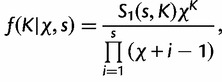
where the term is the prior density on the tree and is the joint prior density over the evolutionary model parameters. Here, we assume prior independence between the tree and evolutionary model parameters. If we apply a coalescent prior to the tree, then is replaced by , where contains the demographic parameters of the coalescent and has hyperprior density . The term is the likelihood given all model parameters. The likelihood at site i, , is calculated by Felsenstein’s pruning algorithm (Felsenstein 1981), and the full likelihood is the product of the likelihood over all sites:

(2)

Heterogeneity of Evolutionary Parameters across Sites

If the evolutionary process is homogeneous across sites then and . To relax this assumption, we estimate an unknown partitioning of the evolutionary model parameters across sites using DPM models.

Consider the SDPM1 model wherein the substitution model parameters and rates share the same partitioning. Let K be an unknown parameter denoting the number of categories of evolutionary model parameters. The substitution model parameters and rate at each site are assigned to one of the K categories. Each category has its own unique set of values of evolutionary model parameters. Let be the union of unique substitution model parameters over all categories, whereas is the union of unique rate multipliers values across all categories. The term denotes the category to which site i has been assigned, where , therefore and . We can rewrite equation (1) in terms of , and , such that

(3)

Under the Dirichlet process,

(4)

where is the number of sites assigned to category k, distributions and are the base distributions of substitution model parameters and rate multipliers, respectively, and is the “concentration parameter” of the Dirichlet process. Notice that permutation of the assignment vector does not affect the distribution in equation (4). Parameter χ controls the marginal distribution on the number of categories a priori:

(5)

where is the absolute value of the Stirling number of the first kind given parameter values s (number of sites) and K. According to equation (5), the Dirichlet process tends to produce more categories with increasing χ.

If the substitution model parameters and rates across sites are modeled by independent Dirichlet processes as in the SDPM2 model, then the full posterior can be written as follows:

(6)

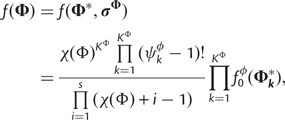
where and are the respective assignment vectors for the substitution model parameters and rates. The prior distribution of substitution model parameters across sites is as follows:

(7)

where is the number of sites assigned to category k of the K^Φ substitution model categories, and is the concentration parameter of the Dirichlet process prior on substitution model partition. The prior distribution of rates across sites follows similarly. We let denote the number of sites in category k of the K^r rate categories and denote the concentration parameter of the Dirichlet process prior on rate partition.

Posterior Inference of Partitioning

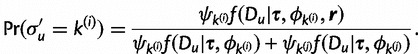
We employ a Gibbs sampling procedure (Neal 2000, algorithm 8) for updating the assignment vector in the SDPM1 model. Site i, which is in category k (), is picked randomly and removed from the rest of the sites. If there are currently K classes, let denote the number of categories after the removal of site i. If site i is an singleton, we create κ auxiliary sets of substitution model parameters and rates by setting to k and draw new parameter values from the base distribution for each of the categories in . If site i is not a singleton, a new set of evolutionary model parameters are drawn for each of the κ auxiliary categories. 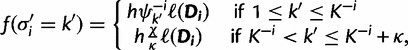The Gibbs sampler proposes a new category, with probability

(8)

where and h is the normalizing constant. Categories are discarded if they are not associated with any site after the update. For the analyses in this study, we use . The same procedure is used to update and in SDPM2.

The Gibbs sampling procedure described above updates the assignment vector site-by-site and therefore lacks efficiency when the number of sites is large because site assignments are highly correlated. To overcome this issue, we also employ a Metropolis–Hastings (Metropolis et al. 1953; Hastings 1970) sampling algorithm that makes updates of assignment at multiple sites in one step by splitting and merging existing categories (Dahl 2005). Using as an example, a sequentially allocated-split-merge sampling has the following steps. We randomly choose a pair of sites i and j, where . If i and j are in the same category k, then k will be split. After removing sites i and j from k, we let denote the set of sites associated with k without i and j. We can then construct two new categories, containing site i and containing site j. We draw one site, u, at a time without replacement from and assign it to with the probability

(9)

The model parameters and are updated by drawing values from their respective base distributions. After each allocation of u, either or increments by 1. The proposal density of splitting a category is the product of equation (9) after each draw from multiplied by . The proposal probability of the reversal step is 1.0, as there is only one assignment option to merge two categories.

If sites i and j are in different categories, kⁱ and k^j, respectively, then they are merged into one category, say k^m. The parameter values associated with this category are set to . The proposal probability of a merge step is 1.0. The reverse proposal probability is multiplied by the product of the probabilities in equation (9) for an assignment choice required to obtain the split allocation to kⁱ and k^j from the merged category k^m.

Bayesian Model Selection

We use a spike-and-slab prior specification (Kuo and Mallick 1998) to facilitate Bayesian selection among named nucleotide substitution models for each category. Under this approach, we augment to include a set of binary indicator variables, whose realized 0, 1 values allow us to move between substitution model parameter restrictions that correspond to common nucleotide models. Specifically, the infinitesimal rate matrix of category k is , where is a symmetric matrix with upper-triangular entries

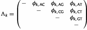(10)

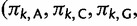
and matrix is diagonal with entries . Using the binary indicators , we further parameterize

(11)

for . Each element of takes a value in the range . The base frequencies satisfy . When certain indicators in achieve the value 0, specific effects fall out of the model. Using this approach, we are able to conveniently parameterize the Kimura (1980, K80), Felsenstein (1981, F81), Hasegawa et al. (1985, HKY85), Tamura and Nei (1993, TN93), and Tavaré (1986, general time reversible [GTR]) infinitesimal rate matrices. Table 1 presents the relationship between and these named models. Also presented in the table 1 is an alternative parameterization of into a single categorical variable achieving five partially ordered values. takes values K80, F81, HKY85, TN93, and GTR. Sampling provides an opportunity to traverse through substitution model space without changing the total model dimension. Finally, the infinitesimal matrix is normalized, so that the total mutational outflow is 1.0; in other words we multiply by .

Table 1.

Indicator Values of a Given Substitution Model.

Indicator
	K80	F81	HKY85	TN93	GTR
	0	1	1	1	1
	1	0	1	1	1
	0	0	0	1	1
	0	0	0	0	1

Single-Locus Data

We applied our method to four single-locus data sets of gene coding sequences, three of which are collected from RNA viruses and one from mammalian species.

Ebola Virus

The Ebola virus (EBOV) data set was compiled by Wertheim and Kosakovsky Pond (2011). It consists of 32 glycoprotein sequences of 1,389 base pairs. The sampling times range from 1976 to 2005.

Hepatitis C Subtype 4

The hepatitis C subtype 4 (HCV-4) data set was data set B in a study on the population genetics and epidemiology history of HCV in Egypt (Pybus et al. 2003). It was originally from a comprehensive study on the diversity of HCV in Egypt (Ray et al. 2000). This data set contains 63 contemporaneous sequences of 411 base pairs from the E1 region.

Mammal

The mammal data set was obtained from the OrthoMam database (Ranwez et al. 2007). The data set contains sequences from 12 mammalian species: Canis familiaris, Felis catus, Homo sapiens, Pan troglodytes, Pongo pygmaeus abelii, Macaca mulatta, Microcebus murinus, Otolemur garnettii, Mus musculus, Rattus norvegicus, Ochotona princeps, and Oryctolagus cuniculus. The sequences have length of 468 base pairs and are from FGF1 gene, which codes for heparin-binding growth factor 1.

Respiratory Syncytial Virus Subgroup A

This data set has 35 sequences and 629 sites from the G gene of the human respiratory syncytial virus subgroup A (RSVA) sampled from 1956 to 2002 (Zlateva et al. 2005).

Hepatitis C Virus Subtype 1b Full-Genome Data

We also analyzed a data set of HCV subtype 1-b genomes used in the study by Gray et al. (2011). It consists of 31 within-host sequences of 9,030 sites sampled between the years 1977 and 2000 inclusive. The main purpose of analyzing this data set is to give a larger multigene example and to compare across-site rate heterogeneity inferred here with the previous study. Therefore, we do not report results for simpler models as we do for the single-locus data sets.

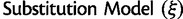
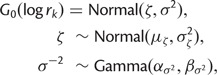
Dirichlet Process Priors

To complete our SDPM1 and SDPM2 construction, we need to specify base distributions for the Dirchlet process(es). When specified hierarchically (Suchard et al. 2003), these distributions allow for the sharing of information across random partitions and the borrowing of strength in parameter estimation. We construct the base distribution for substitution model parameters as . We use a multivariate normal distribution as the base for . To induce a hierarchy, mean and variance are treated as random parameters, where is assumed to have a multivariate normal prior with fixed mean and variance . The precision carries a Wishart prior, with scale matrix V and degrees of freedom d.

We constructed informative priors on and for the analyses on the RNA virus data sets according to the following procedure. We analyzed 26 RNA virus data sets (listed in supplementary table S1, Supplementary Material online) from Jenkins et al. (2002) with using (Guindon et al. 2010, Phyml). models the rate across site with discretized gamma distribution with four categories. The maximum likelihood estimates (MLEs) of the relative rates in the GTR model were transformed to the space of . Using the mclust package in R (Fraley and Raftery 2002, 2006), we fitted a multivariate normal distribution to these estimates across the data sets, yielding and . There is little information on how the variance should vary across sites, so we set and d = 7, so that the prior mean of matches . Informative priors on and for analyses on the mammal data set were also constructed according to the procedure above with 25 mammal data sets (listed in supplementary table S2, Supplementary Material online) randomly selected from Ranwez et al. (2007).

The base distribution of nucleotide base frequencies is formulated as follows:

(12)

where η is the dispersion parameter and is the across-partition mean frequencies. The base distribution of the substitution model indicator is given by

(13)

where are the across-partition model probabilities. Having these hierarchical prior parameters , η and will improve mixing for the partition allocation variables. The parameterization of our Q matrix can also accommodate Jukes et al. (1969, JC69). However, this set up of mixture model treats categories with having different ρ and/or f values as different categories. This is not preferable as these categories have effectively the same model. Therefore, we exclude JC69 from our model to avoid this problem.

The base distribution of rate is assumed to be a lognormal distribution and takes the form

(14)

where ζ is mean and is the variance.

For the analyses on the serially sampled RNA virus data sets (EBOV and RSVA), informative prior on ζ is constructed by fitting a lognormal distribution (Venables and Ripley 2002) to the MLEs of substitution rate across 50 data sets presented in Jenkins et al. (2002). The log-space mean and standard deviation of the fitted lognormal distribution are assigned to and , respectively.

In analyses of contemporaneous sequences (like the mammal and HCV-4 data sets), rate and time cannot be separated without node calibrations. Usually, one would fix the rate to 1.0 and estimate the tree height in substitution units. As our DPM models estimate the rate multipliers, ideally we would like to fix the tree height to 1.0. However, doing so forbids some proposal moves that are important for efficient traversal of tree space. Therefore, we use a narrow normal prior, Normal(1.0, 0.1), on the tree height. This reduces the problem of nonidentifiability and permits useful tree proposals. We assume the log-space mean of the rate base distribution, ζ, is from Normal(–2.3, 2.35). Thus, the median of the base distribution, , is assumed to come from Lognormal(–2.3, 2.35). This lognormal distribution has 2.5%, 50.0% (median), and 97.5% quantiles of 0.001, 0.1, and 10.0, respectively. It is a broad prior that covers the range of relevant tree heights (measured in substitutions per site).

The gamma prior applied to has shape and rate , which is a fairly broad exponential distribution with variance of 100.

Following the analyses presented in model selection method articles of Lemey et al. (2009) and Heled and Drummond (2010), we also place 50% prior probability on the most parsimonious model by setting the χ of SDPM1 and and of SDPM2 to values, such that the prior probability is 0.5 for K = 1 for SDPM1 and K^Φ and K^r for SDPM2.

Analysis

The data sets were analyzed with , SRD2006 ( for each codon position), , SDPM1, and SDPM2. In addition, the data sets were also analyzed using SDPM2 with K^Φ fixed to 1. This special case of the SDPM2 is labeled RDPM (rate Dirichlet mixture model), which is very similar to the model presented by Huelsenbeck and Suchard (2007). The rates across sites are not normalized when using RDPM, SDPM1, or SDPM2.

For each data set and substitution model, we analyze them with a strict clock model and an uncorrelated lognormal relaxed molecular clock (Drummond et al. 2006, LNRC). To extract the absolute site rates (or site tree heights if calibration is absent), the branch rates are normalized to 1.0.

Analyses of all virus data sets used a Bayesian skyline plot coalescent prior (Drummond et al. 2005), whereas the Mammal data set had a Yule process prior.

The first 10% steps of the MCMC are discarded as burn-in. The convergence and quality of mixing was examined by using Tracer v1.5 (Rambaut and Drummond 2009). Supplementary table S3, Supplementary Material online, presents the MCMC chain lengths for each analysis. The marginal likelihood of each analysis was approximated using the method proposed by Newton and Raftery (1994) with the stabilization made by Redelings and Suchard (2005).

All input XML files for the analyses performed and the source code for the BEAST 2 add-on that implements the described methodology are available from http://code.google.com/p/subst-bma/(last accessed December 6, 2012). This add-on consists of 1) priors for model parameters, 2) a suite of proposal moves for sampling the partition via Gibbs and Metropolis–Hastings sampling, 3) extensions to likelihood calculations, and 4) components that enable BEAST 2 to handle a variable number of models during the MCMC.

To infer the posterior distribution of the tree topology, we use a series of proposal moves, including narrow exchange, wide exchange (Drummond et al. 2002), Wilson–Balding (Wilson and Balding 1998), and subtree-slide. Subtree-slide is similar to moves proposed by the LOCAL operator (Mau and Newton 1997; Mau et al. 1999; Larget and Simon 1999). Details of these moves are described in Höhna et al. (2008) and have been implemented in both the BEAST 1 and BEAST 2 software packages.

Simulation Study

Simulated data sets are generated under two procedures. In the first procedure, we randomly drew parameters of a GTR model and the shape parameter α of a Gamma-distributed site rate model from empirically derived distributions fit to the 25 virus data sets as described in the Dirichlet process prior section. We then drew four site-specific rate values from a Gamma distribution with shape set to α. Each site in the alignment was assigned to one of the four rates with equal probability. Using the randomly drawn GTR model and site rates, sequences were simulated on a tree with 30 taxa randomly drawn from a Yule model with a birth rate of 20. Here, the true value of and . One hundred data sets were simulated under this procedure, and each of them is analyzed with RDPM, SDPM1, and SDPM2.

In the second procedure, we randomly drew 100 sets of model partitions and tree from posterior of the HCV-4 data set analyzed with SDPM2 and strict clock model. Sequences were simulated with 411 sites. These data sets are analyzed with SDPM2.

The priors on the hyperparameters of Dirichlet process base measure are the same as those used for analyzing HCV-4 data set. In all simulation analyses, we fixed the concentration parameter to the value that gave rise to prior probability of 0.5 for K/K^Φ/K^r= 1. We then repeated all the simulation analyses but allowed the concentration parameter to be estimated. We assumed

(15)

where the rate, γ, was set to a value, such that the prior probability is 0.5 for K/K^Φ/K^r= 1. γ therefore was set to 0.135 for the simulated sequences with 1,000 sites and 0.154 for those with 411 sites.

Results

Heterogeneity in Substitution Patterns

The posterior distributions of the number of category parameters K, K^Φ, and K^r provide some indication of the level of heterogeneity in the substitution process across sites. Figure 1 presents the posterior distributions of K, K^Φ, and K^r, as well as their prior distribution in each mixture model analysis. Although each of K, K^Φ, and K^r takes the value 1 with prior probability of 0.5, most analyses exclude K = 1 when analyzed with SDPM1 and exclude and when analyzed with SDPM2 from their respective 95% highest posterior density (HPD) intervals, providing strong evidence for heterogeneity of substitution pattern and rates across sites. The only exceptions are the K^Φ estimates for the RSVA data set. The Bayes factor for across-site homogeneity versus heterogeneity of substitution patterns is given by

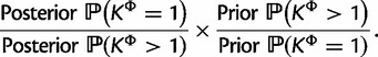(16)

Fig. 1.

Posterior distributions of the number of categories for substitution pattern and rates from analyses with mixture models. The prior distribution of the number of categories is in brown. The posterior distribution of K estimated using SDPM1 is in orange. The posterior distributions of K^Φ and K^r estimated using SDPM2 are colored in green and purple, respectively.

For RSVA, the Bayes factor is 0.140 for the strict clock analysis and 0.175 for the relaxed clock analysis. While far from definitive, these Bayes factors provide substantial evidence against across-site homogeneity in substitution pattern according to the interpretation scale provided by Jeffreys (1998). A more conclusive outcome may be obtained by adding more sequences. Conditioned on the data set and clock model, the estimated posterior means of K^Φ and K^r are smaller than that of K, which suggests that less categories of substitution pattern are required if the site rate heterogeneity is modeled separately. However, there is one exception—for EBOV, the posterior mean of K^Φ is not smaller than that of K (supplementary table S4, Supplementary Material online).

One question of interest is “Should every site in an alignment be modeled by the same type of nucleotide substitution model?” If not, it is important to infer which substitution model should be used at each site. We present the answer obtained from the DPM model analyses in figure 2, which consists of 16 grid plots. In each grid plot, each row represents one of the five nucleotide substitution models and each column represents a site in an alignment. A grid located in row M and column i is colored according to the posterior probability of site i being generated by model M. The color darkens as the probability increases. The posterior average number of sites that have selected an M model is on the right side of the plot. Given a data set and an SDPM model, little difference is seen in the across-site substitution pattern between strict clock and LNRC analyses. However, there appears to be some differences between SDPM1 and SDPM2 analyses. In the SDPM1 analyses on EBOV, there seems to be some support for F81; however, this is not evident after switching to SDPM2 as illustrated by the white band in the F81 row. An even larger contrast is displayed by the analyses on HCV-4. The results from the SDPM1 analyses on HCV-4 suggest that the most favored model is K80; however, the SDPM2 analyses show almost no support for K80 and clear preference for TN93 and GTR. All SDPM analyses on Mammal prefer K80, but this seems stronger in the SDPM1 analyses. In contrast, the reverse pattern is observed in the analyses on RSVA, where all analyses prefer GTR, but the preference is stronger in the SDPM2 analyses.

Fig. 2.

Support for each model at each site indicated by the posterior probability that a model is selected to fit that site. The color becomes darker as the posterior probability increases. The average number of sites fitted by a model is indicated on the axes on the right hand side of the plots.

Figure 2 does not provide information on whether two sites i and j, which both prefer a specific type of model, are modeled by the same parameter values. That is, if site i prefers a GTR model it does not follow that site, j also prefers the same GTR parameter values. To illustrate the cluster structure, we performed cluster analyses on the estimates of substitution model parameters using k-means algorithm implemented in the R package MASS (Venables and Ripley 2002; R Development Core Team 2011). Let , and represent estimated posterior mode of K, K^Φ, and K^r, respectively. The number of clusters is predefined in the algorithm. Cluster analyses on SDPM1 parameter estimates have K_max clusters, whereas those on SDPM2 parameter estimates have . As examples, we present the results from the cluster analyses for the mammal (fig. 3) and RSVA (fig. 4). Figure 3 shows that sites are indeed clustered according to the model most preferred. Those that have chosen K80 tend to be in one cluster, and those prefer F81 is in another cluster. This segregation does not appear in the results for RSVA (fig. 4). Although most sites prefer the GTR model, there is still grouping structure, in other words, they are not modeled by the same GTR.

Fig. 3.

Support for substitution models at each site of the Mammal data set, with each site colored according to the cluster to which it is assigned by the cluster analysis performed on the estimates of substitution model parameters. For the SDPM1 analyses, the sites are grouped into four clusters as the marginal posterior probability of K is the largest when K = 4 and the colors used to distinguish them are blue, green, purple, and orange. For the SDPM2 analyses, has the largest marginal posterior probability, so the sites are grouped into two clusters colored with blue and orange. The posterior probability is indicated by the darkness of the color in part (a). Darker coloring corresponds to higher probability. Only the model with the highest posterior probability (best model) at each site is colored in part (b), and the number of sites that selects a model as the best model is reported on the axis on the right hand side.

Fig. 4.

Support for substitution models at each site of the RSVA data set, with each site colored according to the cluster to which it is assigned by the cluster analysis performed on the estimates of substitution model parameters. The posterior mode values of K and are equal to two; therefore, for both SDPM1 and SDPM2 analyses, sites are grouped into two clusters colored blue and red. The posterior probability is indicated by the darkness of the color in part (a). Darker coloring corresponds to higher probability. Only the model with the highest posterior probability (best model) at each site is colored in part (b), and the number of sites that selects a model as the best model is reported on the axis on the right hand side.

Because all data sets used in this study code for proteins, we would like to see whether the across-site heterogeneity in rate uncovered by our mixture models corresponds to codon positions. For each MCMC step that has categories, we first order the categories in increasing order of the rate, so that category 1 has the slowest rate, whereas category has the fastest rate. The proportion of sites in each category is computed for each codon position. The same procedure is repeated for the results from SDPM2 analyses, except is replaced by , the number of rate categories with the highest posterior probability. Figure 5 illustrates the posterior mean proportions of sites in category 1 to category for every SDPM1 analysis and the posterior mean proportions in category 1 to for every SDPM2 analysis. The bars are colored according to the proportion of sites in each category, and the category with a faster rate is closer to the top of the bar. All analyses show that in general the third codon position has a higher substitution rate, although there is much variation within the codon positions. This increase in the third codon rate is concordant with previous findings (Huelsenbeck and Suchard 2007).

Fig. 5.

Proportion of sites in each codon position as a function of rate. The number of category shown has the maximum posterior probability. Each bar represents a codon position, and it is colored according to the posterior mean proportion of sites in each rate category. The colors are picked from the “rainbow” scheme, and clusters with faster mean rate are in colors closer to the violet end.

We examine whether the preference for the type of substitution model also differs by codon position. For each state, we compute the proportion of sites at each codon position selecting each one of the five types of substitution model. The posterior mean proportions for each codon position are presented in the plots shown in supplementary figure S1, Supplementary Material online. SDPM1 analyses show that the preference for the type of substitution model seems to differ by codon positions. For EBOV, HCV-4, and Mammal, sites in the third codon position appear to prefer more complex substitution models, but the difference is not so apparent in the RSVA data set. In contrast, the SDPM2 analyses do not show any significant difference in preference for substitution models across codon positions.

We compute the relative standard deviation (RSD) for the substitution model parameter values across the categories. RSD is the standard deviation divided by the absolute value of the mean. The values of posterior mean and 95% credible interval boundaries of RSD are presented in figure 6. Analyses with SDPM1 on EBOV produce relative rate parameters with mean RSD values around 1, except for the rate between C and T. Analyses on HCV-4 and mammal produce mean RSD values around 1 for relative rates, other than that between C and T. These RSD values suggest reasonably clear signal of heterogeneity in substitution pattern, which is likely to have contributed to the difference in model choice across sites as shown in figure 2. All posterior mean RSD values estimated from RSVA are between 0.15 and 0.7, which are generally lower than those produced by other data sets. It suggests that the signal for heterogeneity in substitution patterns is not strong. Moreover, it is consistent with a higher posterior probability for homogeneity in this data set than others.

Fig. 6.

Posterior RSD of substitution model parameter values across categories. Analyzed with SDPM1 are in red, SDPM2 in blue, strict clock model in solid lines, and lognormal relaxed clock model in dotted lines.

Model Comparison

The Bayes factor is often used for model comparison in Bayesian analysis, expressing the ratio of the marginal likelihoods of two competing models. The marginal likelihood is the likelihood of the data given the model and is integrated across the entire parameter space of the model. It therefore accounts for the complexity of the model and penalizes greater model complexity. The natural logarithm of the marginal likelihoods of all single-locus analyses are presented in table 2, and their differences are log Bayes factors.

Table 2.

The Natural Log Marginal Likelihoods of Analyses with Strict Clock Model.

Data Set	Clock Model	HKY+	GTR	SRD2006	GY94I	RDPM	SDPM1	SDPM2
EBOV	SC	−7,495	−7,487	−7,114	−6,734	−6,914	−6,682	−6,531
EBOV	LNRC	−7,479	−7,468	−7,093	−6,714	−6,892	−6,648	−6,475
HCV-4	SC	−6,172	−6,167	−6,041	−6,208	−5,860	−5,638	−5,601
HCV-4	LNRC	−6,153	−6,147	−6,017	−6,190	−5,814	−5,596	−5,550
Mammal	SC	−1,695	−1,689	−1,582	−1,522	−1,570	−1,534	−1,517
Mammal	LNRC	−1,690	−1,681	−1,578	−1,518	−1,565	−1,523	−1,511
RSVA	SC	−3,112	−3,093	−3,072	−3,132	−2,995	−2,988	−2,979
RSVA	LNRC	−3,108	−3,091	−3,068	−3,130	−2,987	−2,987	−2,976

The substitution models are of increasing complexity from left to right. Conditioned on a data-clock model combination, the worst fit to the data is found in nucleotide substitution models that do not account for across-site heterogeneity in substitution patterns and do not estimate rate partitioning. Allowing restricted heterogeneity by performing codon partition substantially improves the marginal likelihood for all data sets except for RSVA. Increasingly flexible partition schemes of the substitution pattern improve the fit of the model substantially. This outcome indicates that codon partitioning does not fully characterize the complexities of across site variation in protein coding sequence alignments.

The fit of relative to other models varies considerably across different data sets. For the Mammal data set, fits the data just, as well as the SDPM models. Similarly, the SDPM models do not fit EBOV substantially better than the codon model. The detected heterogeneity of these two data sets may therefore be just as easily explained by a simple codon-based model. However, the codon model does not fit the RSVA and HCV-4 data sets, as well as the SDPM models. For those two data sets, the SDPM models have substantially better marginal likelihoods than all the other substitution models. This suggests that the heterogeneity in these two protein coding sequences cannot be fully explained by the genetic code or at least the properties of the genetic code incorporated in codon model tested here.

For the data sets HCV-4, Mammal, and RSVA, the difference in the marginal likelihood between SDPM1 and SDPM2 is natural log units. However, for EBOV, the difference is natural log units and the log marginal likelihood difference between SDPM1 and SDPM2 is 16–19 times the difference between HKY and GTR. Therefore, the improvement in model fit of SDPM2 over SDPM1 can sometimes be very substantial.

Estimation of Phylogenetic Parameters and Their Hyperparameters

The tree height estimates are shown in figure 7. Given a clock model, the mixture models tend to produce older trees than other simpler substitution model partitions for EBOV. The estimated posterior means of the EBOV tree height under SDPM models are between 51% and 61% older than that of other nucleotide models for strict clock analyses and are between 40% and 62% older for relaxed clock analyses. The codon model analyses and SDPM analyses have similar tree height estimates. The results from the strict clock analyses on HCV-4 show that the tree height estimates of SDPM models are, in contrast, 34–52% shorter than that of other models. Moreover, the SDPM models produced even shorter trees (68–78% shorter) in LNRC analyses than in strict clock analysis. However, the difference in tree length estimates is much smaller between DPM models and others. The posterior mean tree length is between 3.53 and 3.97 for SDPM models and 4.41 and 4.83 for non-SDPM models. This suggests that the SDPM models only reduced the lengths of a few branches in the trees near the root. The analysis with the model produced a much taller Mammal tree than all nucleotide substitution models, among which the tree height estimates do not display substantial differences. For the RSVA data set, the tree height estimates do not vary significantly across all substitution models given a strict clock model.

Fig. 7.

Tree height estimates. Each bar spans the 95% HPD of the tree height, and the posterior mean is marked on the bar. Solid bars are estimates from strick clock analyses, whereas the dashed bars are estimated from the lognormal relaxed clock analyses.

To ease tree-space visualization, we have subsampled 100 trees from each posterior tree distribution. For the 700 trees obtained from the same clock model and data set, we compute the Robinson-Foulds distance between each tree. We apply principle coordinate analysis (PCO) on the 700 × 700 distance matrices. Supplementary figure S2, Supplementary Material online, presents the reduced-space plots with the scores on the first two major principle axes. Each point represents a tree from the subsample. Of the four data sets, only the posterior distributions of HCV-4 produced reduced-space plots that displayed clustering by site model (each model was distinguished by a different color) (fig. 8). There appears to be three major groupings by model: (green) stands out as a single model; the SDPM1 (blue) and SDPM2 (purple) seem clearly separated from the common nucleotide substitution models, (red), (orange), and SRD2006 (yellow). RDPM (turquoise) scatters between SDPMs and the common nucleotide substitution models. It is natural that RDPM bridges the two groupings as it does not partition the alignment for substitution models, but it does estimate the substitution model and across-site rate variation with a DPP.

Fig. 8.

Reduced space of substitution models based on clade posterior probability estimated from HCV-4. Each point represents a tree from the subsample. The trees are colored according substitution model used in the analysis. is colored red, orange, SRD2006 yellow, green, RDPM turquoise, SDPM1 blue, and SDPM2 purple.

To further investigate the differences in tree topology of HCV-4, we record all the unique clades and their posterior probability in each of the two posterior tree distributions. Conditioned on a clock model, each substitution model has a vector of posterior probabilities for each clade. We use clade posterior probabilities to find the Manhattan distance between each pair of substitution model parameters. A 7 × 7 distance matrix is constructed for the substitution models. A PCO analysis is performed on this distance matrix, and the reduced-space plots with the first two major PAs are presented in figure 9.

Fig. 9.

Reduced space of substitution models based on clade posterior probability.

The same groupings appear again in these plots. For each clade, we find the range (max–min) of posterior probabilities across the seven substitution models. The top 50 clades with the highest range of posterior probability have range values between 0.278 and 0.882 for strict clock analysis and between 0.258 and 0.793 for relaxed clock analysis. Difference in clade support indicates that different substitution models support different topologies. We select , and SDPM2 as representatives of each cluster. The top 50 clades with the highest range of posterior probability are mapped to the maximum clade credibility trees of HCV-4 produced by those substitution models (supplementary figs. S3–S8, Supplementary Material online).

To provide some indication on how the posterior distribution on tree topology differs across the different substitution models, supplementary table S5, Supplementary Material online, presents the 95% credible tree sets and the 50% and 5% credible clade sets.

The Bayesian skyline plots for the virus data sets are presented in figure 10. The discrepancies in the tree height estimates of a given data set are reflected in the time frame of the BSPs. For EBOV, the population size estimates produced by the DPM models are much larger at a given time than those produced by other across-site substitution-rate models in both strict clock analyses and relaxed clock analyses. However, all the across-site substitution-rate models shares the same pattern in how population changes over time—they all show that the population of the EBOV is constant up to approximately 100 years ago followed by a bottleneck. The population size estimates and time frame have been rescaled for the results on HCV-4 by using a previously estimated substitution rate (Pybus et al. 2001). The BSPs from the strict clock analyses shows that population sizes are quite similar across all substitution models. This suggests that the population size of HCV-4 in Egypt was constant until a rapid expansion occurred approximately 60 years before sample collection. However, the LNRC analyses with the mixture models on HCV-4 suggest a slightly earlier expansion date than other relaxed clock analyses. Given a strict clock model, BSPs estimated for RSVA are very similar across all across-site substitution-rate models.

Fig. 10.

Bayesian skyline plots for the analyses on EBOV, HCV-4, and RSVA. Each plot presents BSPs estimated under HKY+Γ+I (red), GTR+Γ+I (orange), SRD2006 (yellow), GY94+Γ+I (green), RDPM (turquoise), SDPM1 (blue) and SDPM2 (purple) for a given data set and clock model.

The 95% HPD intervals and the estimated posterior mean of the birth rate of the Yule process prior are very similar across all analyses with nucletode substitution models on Mammal. The lower bound the 95% HPD interval is between 9.22 and 11.48, whereas the upper bound is between 33.34 and 38.29. The posterior mean ranges from 20.56 to 22.38. This indicates that the inference on birth rate is not affected by the choice of nucleotide substitution model in this case. Birth rate estimates inferred from are much lower. The strict clock analysis estimates a posterior mean (95% HPD interval) of 14.6 (5.87–23.5), which is similar to that inferred from the LNRC analysis 15.0 (6.07–25.7).

Hepatitis C Virus Subtype 1b Full-Genome Data

Figure 11 displays the 95% HPD intervals of site-specific rates from the RDPM + LNRC analysis on HCV-1b genome sequences. The rest of the results from RDPM and SDPM1 analyses are presented in supplementary figure S9, Supplementary Material online. Comparing with Figure 1(a) from Gray et al. (2011), our results also show a hot spot around 1,250th site, whereas the rate is fairly uniform across the rest of the genome. This is probably why the entire genome (HCV-1b) does not require many more rate categories (supplementary table S4, Supplementary Material online) than the E1 gene sequences (HCV-4). The region with the unusually fast rates is near the border of genes E1 and E2. The plots also suggest that sites at the third codon position have higher rates (long blue upper tails) than others. In addition, supplementary figure S9, Supplementary Material online, shows less variation in rate estimates inferred from SDPM1 model. This could be due to decreased sensitivity because the SDPM1 model does not allow separation of rate and pattern heterogeneity.

Fig. 11.

The 95% HPD intervals of site-specific rates for the HCV-1b genome sequences. Codon positions 1, 2 and 3 are coded in red, green, and blue, respectively.

Simulations

Averaged values of statistics used to indicate accuracy and precision of our method are presented in table 3. As measures of accuracy, we use relative bias and the frequency of the true value inside the 95% HPD interval. Relative error and relative size of the 95% HPD interval are used to indicate the level of precision. If a data set is generated with K categories, the relative bias is given by where is the posterior mean of K estimated from a simulated data set. The relative error is the absolute value of the relative bias. If the 95% HPD interval of K has upper () and lower bounds (), the relative size of 95% HPD interval is defined as .

Table 3.

Statistics of Accuracy and Precision of the Estimate of the Number of Categories.

Data Simulation Procedure	Model	Parameter	Estimate χ	Relative Bias	Relative Error	% Inside 95% HPD Interval	Relative 95% HPD Interval Size
One	RDPM	Kr	N	−0.310	0.310	1.00	0.790
			Y	−0.0409	0.122	1.00	1.49
	SDPM1	K	N	−0.306	0.306	1.00	0.810
			Y	−0.0178	0.147	1.00	1.52
	SDPM2	KΦ	N	0.693	0.693	0.98	3.09
			Y	0.885	0.885	1.00	4.23
		Kr	N	−0.307	0.307	0.99	0.795
			Y	−0.0612	0.138	1.00	1.45
Two	SDPM2	KΦ	N	−0.237	0.243	0.61	0.531
			Y	0.140	0.179	1.00	1.15
		Kr	N	−0.138	0.221	0.92	1.14
			Y	−0.105	0.266	1.00	1.81

For all data sets simulated, we generally underestimated the number of rate categories, which is not surprising as the prior strongly favors homogeneity. However, the negative bias is reduced substantially if we estimate the concentration parameter. This may be attributed to the longer tails of the prior distribution on the number of categories when χ is estimated (supplementary fig. S10, Supplementary Material online). RDPM does not estimate the number of substitution model categories. As for SDPM1, the substitution model and rate share the same category structure. The K^Φ estimates from the first set of simulations are naturally positive biased as the true K^Φ value is the lower bound (1). The K^Φ estimates from the second set of simulations tend to be negatively biased if the concentration parameter value is fixed. If we estimate the concentrating parameter value, then estimates of K^Φ seem positively biased with smaller magnitude.

Analyses on data sets simulated from the first procedure yielded high 95% HPD coverage of the true number of categories (0.98–1.00). For data sets simulated from the second procedure, HPD coverage is also high for the true number of categories except for K^Φ when the concentration parameter is fixed. This is attributed to the strong negative bias of the estimate, when the true number of categories is large.

For both the number of rate and substitution pattern categories, it appears that the size of relative 95% credible interval is smaller when the value of concentration parameter is fixed than when it is estimated. This outcome is expected as estimating the concentration parameter creates greater uncertainty in the prior on the number of categories.

Discussion

We have presented DPM models that accommodate across-site heterogeneity in both nucleotide substitution pattern and rate. Using Dirichlet process priors enables the estimation of the number of categories required to explain the heterogeneity of nucleotide substitution, as well as the site-to-category assignment. This obviates a priori specification of the partitioning scheme before the analysis. Because the partitioning is carried out at the nucleotide level, our method is more flexible and is not limited to protein coding alignments. More importantly, sites are grouped together based on the similarity of their substitution properties (substitution model or rate parameters) as informed by the data itself.

Similar to previously proposed models that also attempt to accommodate across-site heterogeneity in nucleotide substitution pattern (Huelsenbeck and Nielsen 1999; Pagel and Meade 2004; Shapiro et al. 2006; Whelan 2008), analyses with our DPM models provide evidence supporting the presence of substitution pattern heterogeneity. The SDPM models also reveal that not all sites favor the same type of nucleotide substitution model in our alignment data. These models seem to be able to capture the codon structure in protein coding sequences as evidenced by the tendency to favor faster rate categories in the third codon position. However, it is also clear that there is rate variation among the sites in the same codon position, therefore the pattern of rate variation is more complex than simple codon partitioning.

In some cases, the phylogenetic and hyperparameter estimates produced by the SDPM models are different to those produced by simpler substitution models. For example, the tree height estimates for EBOV produced by the DPM models are substantially older than when using simpler models but similar to that produced by a codon substitution model (Wertheim and Kosakovsky Pond 2011). Perhaps, the heterogeneity found in the data set is the result of selection pressure; however, uncovering the cause of across-site substitution heterogeneity is beyond the scope of this study. The data sets that exhibit significant differences in phylogenetic estimates between DPM model analyses and others also displayed higher levels of across-site heterogeneity in substitution patterns. However, to confirm this trend, a more comprehensive study is required.

The SDPM models fit our four single-locus data sets far better than all standard nucleotide substitution models tested. This is compatible with the presence of across-site heterogeneity of the substitution pattern in the data sets explored. In addition, the large improvement in model fit obtained by SDPM models suggest that simple codon models are not always adequate for protein coding sequences. Our results show that the SDPM models can substantially outperform codon models. As a large prior weight (probability of 0.5) is placed on across-site substitution homogeneity, the variation detected is likely to represent strong evidence of a real signal of site heterogeneity. Because SDPM models can have a large number of parameters (eight free parameters per substitution model category), if the data set is small then overfitting may occur. Overfitting can be prevented by setting the concentration parameter of the Dirichlet process to a smaller value, favoring fewer categories. The substitution model is parameterized, so that the substitution model of each category can be “estimated,” achieving site to model assignment. The set of substitution models for selection include models that aim to capture the biological properties observed in nucleotide substitution.

It is quite possible that the most suitable model for a particular (set of) site(s) is not in the set of substitution models we have specified. Fine tuning the set of substitution models may improve the quality of fit. In the model selection study by Huelsenbeck et al. (2004), they have exploited the entire space of 203 possible nucleotide substitution models. Although the most favored models were unnamed ones, in their study they found that the predominant pattern is the difference in the rate between transition and transversion. Moreover, this appears to be the decisive factor for whether or not a model has the highest posterior probability. The models with the highest posterior probability appeared to only have minor difference to named models such as Kimura (1980); Hasegawa et al. (1985). Although most of the favored/best models are unnamed, they still conform to the biological behavior that the standard named models aim to capture/parameterize. Because the differences between the unnamed best model and standard named models are likely to be minor, there should not be drastic differences in the quality of the fit. The relatively small differences in marginal likelihood between HKY and GTR models, when compared with the large differences between them and the SDPM models suggest that modeling improvements that capture rate and pattern heterogeneity across sites will dwarf any gains that might be achieved by providing for intermediate substitution models.

A future improvement of our method is to relax the definition of units of category assignments. Currently, alignment sites are the units of category assignments. If we allow the units to be genes, it may be useful for phylogenomic analyses. In this study, we have not explored the entire substitution model space and have not allowed variation in the topology across partitions. Incorporating either of these properties substantially expands the parameter space, and carefully devised proposal moves would be required to traverse this expanded space. Hence, these extensions are outside the scope of this study but are both potential research directions worth exploring.

The phylogenetic and hyperparameter estimates produced by SDPM analyses are averaged over the alignment partition space of rates and substitution pattern. These estimates therefore take into account the uncertainty associated with alignment partitioning. The user can therefore bypass the process of model and partition selection. Conversely, if one is interested in the across-site heterogeneity in the substitution process, our method can provide relevant information. Furthermore, it is clear from the large improvements in model fit that our approach goes some way to solving the problem of site to model assignment. We think that the methods described here provide a superior approach that can replace existing widely used methodologies for substitution model comparison and selection.

Supplementary Material

Supplementary figures S1–S10 and tables S1–S5 are available at Molecular Biology and Evolution online (http://www.mbe.oxfordjournals.org/).

References

- Antoniak CE. Mixtures of Dirichlet processes with applications to Bayesian nonparametric problems. Ann Stat. 1974;2:1152–1174. [Google Scholar]
- Bruno WJ. Modeling residue usage in aligned protein sequences via maximum likelihood. Mol Biol Evol. 1996;13:1368–1374. doi: 10.1093/oxfordjournals.molbev.a025583. [DOI] [PubMed] [Google Scholar]
- Churchill GA, von Haeseler A, Navidi WC. Sample size for a phylogenetic inference. Mol Biol Evol. 1992;9:753–769. doi: 10.1093/oxfordjournals.molbev.a040757. [DOI] [PubMed] [Google Scholar]
- Dahl D. Technical report. Madison (WI): Department of Statistics, University of Wisconsin–Madison; 2005. Sequentially allocated merge-split sampler for conjugate and nonconjugate Dirichlet process mixture models. [Google Scholar]
- Dimmic M, Mindell D, Goldstein R. Modeling evolution at the protein level using an adjustable amino acid fitness model. Pac Symp Biocomput. 2000;5:18–29. doi: 10.1142/9789814447331_0003. [DOI] [PubMed] [Google Scholar]
- Drummond A, Nicholls G, Rodrigo A, Solomon W. Estimating mutation parameters, population history, and genealogy simultaneously from temporally spaced sequence data. Genetics. 2002;161:1307–1320. doi: 10.1093/genetics/161.3.1307. [DOI] [PMC free article] [PubMed] [Google Scholar]
- Drummond AJ, Ho SYW, Phillips MJ, Rambaut A. Relaxed phylogenetics and dating with confidence. PLoS Biol. 2006;4:e88. doi: 10.1371/journal.pbio.0040088. [DOI] [PMC free article] [PubMed] [Google Scholar]
- Drummond AJ, Rambaut A, Shapiro B, Pybus OG. Bayesian coalescent inference of past population dynamics from molecular sequences. Mol Biol Evol. 2005;22:1185–1192. doi: 10.1093/molbev/msi103. [DOI] [PubMed] [Google Scholar]
- Felsenstein J. Evolutionary trees from DNA sequences: a maximum likelihood approach. J Mol Evol. 1981;17:368–376. doi: 10.1007/BF01734359. [DOI] [PubMed] [Google Scholar]
- Felsenstein J. Sunderland (MA): Sinauer Associates; 2004. Inferring phylogenies. [Google Scholar]
- Ferguson TS. A Bayesian analysis of some nonparametric problems. Ann Stat. 1973;1:209–230. [Google Scholar]
- Fraley C, Raftery AE. Model-based clustering, discriminant analysis, and density estimation. J Am Stat Assoc. 2002;97:611–631. [Google Scholar]
- Fraley C, Raftery AE. Seattle (WA): Department of Statistics, University of Washington; 2006. Mclust version 3 for R: normal mixture modeling and model-based clustering. Technical Report 504. [Google Scholar]
- Godsill SJ. On the relationship between Markov chain Monte Carlo methods for model uncertainty. J Comput Graph Stat. 2001;10:230–248. [Google Scholar]
- Golding G. Estimates of DNA and protein sequence divergence: an examination of some assumptions. Mol Biol Evol. 1983;1:125–42. doi: 10.1093/oxfordjournals.molbev.a040303. [DOI] [PubMed] [Google Scholar]
- Goldman N, Thorne JL, Jones DT. Assessing the impact of secondary structure and solvent accessibility on protein evolution. Genetics. 1998;149:445–458. doi: 10.1093/genetics/149.1.445. [DOI] [PMC free article] [PubMed] [Google Scholar]
- Gray R, Parker J, Lemey P, Salemi M, Katzourakis A, Pybus O. The mode and tempo of hepatitis C virus evolution within and among hosts. BMC Evol Biol. 2011;11:131. doi: 10.1186/1471-2148-11-131. [DOI] [PMC free article] [PubMed] [Google Scholar]
- Green PJ. Reversible jump Markov chain Monte Carlo computation and Bayesian model determination. Biometrika. 1995;82:711–732. [Google Scholar]
- Gu X, Fu YX, Li WH. Maximum likelihood estimation of the heterogeneity of substitution rate among nucleotide sites. Mol Biol Evol. 1995;12:546–557. doi: 10.1093/oxfordjournals.molbev.a040235. [DOI] [PubMed] [Google Scholar]
- Guindon S, Dufayard J, Lefort V, Anisimova M, Hordijk W, Gascuel O. New algorithms and methods to estimate maximum-likelihood phylogenies: assessing the performance of phyml 3.0. Syst Biol. 2010;59:307–321. doi: 10.1093/sysbio/syq010. [DOI] [PubMed] [Google Scholar]
- Hasegawa M, Kishino H, Yano T. Dating of the human-ape splitting by a molecular clock of mitochondrial DNA. J Mol Evol. 1985;22:160–174. doi: 10.1007/BF02101694. [DOI] [PubMed] [Google Scholar]
- Hastings WK. Monte Carlo sampling methods using Markov chains and their applications. Biometrika. 1970;57:97–109. [Google Scholar]
- Heled J, Drummond A. Bayesian inference of species trees from multilocus data. Mol Biol Evol. 2010;27:570–580. doi: 10.1093/molbev/msp274. [DOI] [PMC free article] [PubMed] [Google Scholar]
- Höhna S, Defoin-Platel M, Drummond A. 2008. Clock-constrained tree proposal operators in Bayesian phylogenetic inference. Proceedings of the 8th IEEE International Conference on Bioinformatics and bioengineering, BIBE; 2008 October 8–10; Athens (Greece). p. 1–7. [Google Scholar]
- Huelsenbeck JP, Hillis DM. Success of phylogenetic methods in the four-taxon case. Syst Biol. 1993;42:247–264. [Google Scholar]
- Huelsenbeck JP, Jain S, Frost SWD, Pond SLK. A Dirichlet process model for detecting positive selection in protein-coding DNA sequences. Proc Natl Acad Sci U S A. 2006;103:6263–6268. doi: 10.1073/pnas.0508279103. [DOI] [PMC free article] [PubMed] [Google Scholar]
- Huelsenbeck JP, Joyce P, Lakner C, Ronquist F. Bayesian analysis of amino acid substitution models. Philos Trans R Soc Lond B Biol Sci. 2008;363:3941–3953. doi: 10.1098/rstb.2008.0175. [DOI] [PMC free article] [PubMed] [Google Scholar]
- Huelsenbeck JP, Larget B, Alfaro ME. Bayesian phylogenetic model selection using reversible jump Markov chain Monte Carlo. Mol Biol Evol. 2004;21:1123–1133. doi: 10.1093/molbev/msh123. [DOI] [PubMed] [Google Scholar]
- Huelsenbeck JP, Nielsen R. Variation in the pattern of nucleotide substitution across sites. J Mol Evol. 1999;48:86–93. doi: 10.1007/pl00006448. [DOI] [PubMed] [Google Scholar]
- Huelsenbeck JP, Suchard MA. A nonparametric method for accommodating and testing across-site rate variation. Syst Biol. 2007;56:975–987. doi: 10.1080/10635150701670569. [DOI] [PubMed] [Google Scholar]
- Jeffreys H. New York: Oxford University Press; 1998. Theory of probability. [Google Scholar]
- Jenkins G, Rambaut A, Pybus O, Holmes E. Rates of molecular evolution in RNA viruses: a quantitative phylogenetic analysis. J Mol Evol. 2002;54:156–165. doi: 10.1007/s00239-001-0064-3. [DOI] [PubMed] [Google Scholar]
- Jin L, Nei M. Limitations of the evolutionary parsimony method of phylogenetic analysis. Mol Biol Evol. 1990;7:82–102. doi: 10.1093/oxfordjournals.molbev.a040588. [DOI] [PubMed] [Google Scholar]
- Jukes T, Cantor C, Munro H. Mammalian protein metabolism. Evol Protein Mol. 1969;3:21–132. [Google Scholar]
- Kimura M. A simple method for estimating evolutionary rates of base substitutions through comparative studies of nucleotide sequences. J Mol Evol. 1980;16:111–120. doi: 10.1007/BF01731581. [DOI] [PubMed] [Google Scholar]
- Koshi JM, Mindell DP, Goldstein RA. Using physical-chemistry-based substitution models in phylogenetic analyses of HIV-1 subtypes. Mol Biol Evol. 1999;16:173–179. doi: 10.1093/oxfordjournals.molbev.a026100. [DOI] [PubMed] [Google Scholar]
- Kuo L, Mallick B. Variable selection for regression models. Sankhya Indian J Stat Ser B (1960–2002). 1998;60:65–81. [Google Scholar]
- Lanfear R, Calcott B, Ho S, Guindon S. Partitionfinder: combined selection of partitioning schemes and substitution models for phylogenetic analyses. Mol Biol Evol. 2012;29:1695–1701. doi: 10.1093/molbev/mss020. [DOI] [PubMed] [Google Scholar]
- Larget B, Simon D. Markov chain Monte Carlo algorithms for the Bayesian analysis of phylogenetic trees. Mol Biol Evol. 1999;16:750–759. [Google Scholar]
- Lartillot N, Philippe H. A Bayesian mixture model for across-site heterogeneities in the amino-acid replacement process. Mol Biol Evol. 2004;21:1095–1109. doi: 10.1093/molbev/msh112. [DOI] [PubMed] [Google Scholar]
- Lemey P, Rambaut A, Drummond A, Suchard M. Bayesian phylogeography finds its roots. PLoS Comput Biol. 2009;5:e1000520. doi: 10.1371/journal.pcbi.1000520. [DOI] [PMC free article] [PubMed] [Google Scholar]
- Li P, Goldman N. Using protein structural information in evolutionary inference: transmembrane proteins. Mol Biol Evol. 1999;16:1696–1710. doi: 10.1093/oxfordjournals.molbev.a026083. [DOI] [PubMed] [Google Scholar]
- Mau B, Newton M. Phylogenetic inference for binary data on dendograms using Markov chain Monte Carlo. J Comput Graph Stat. 1997:122–131. [Google Scholar]
- Mau B, Newton M, Larget B. Bayesian phylogenetic inference via Markov chain Monte Carlo methods. Biometrics. 1999;55:1–12. doi: 10.1111/j.0006-341x.1999.00001.x. [DOI] [PubMed] [Google Scholar]
- Metropolis N, Rosenbluth AW, Rosenbluth MN, Teller AH, Teller E. Equation of state calculations by fast computing machines. J Chem Phys. 1953;21:1087. [Google Scholar]
- Neal RM. Markov chain sampling methods for Dirichlet process mixture models. J Comput Graph Stat. 2000;9:249–265. [Google Scholar]
- Newton MA, Raftery AE. Approximate Bayesian inference with the weighted likelihood bootstrap. J Royal Stat Soc Ser B. 1994;56:3–48. [Google Scholar]
- Nielsen R. Site-by-site estimation of the rate of substitution and the correlation of rates in mitochondrial DNA. Syst Biol. 1997;46:346–353. doi: 10.1093/sysbio/46.2.346. [DOI] [PubMed] [Google Scholar]
- Olsen G. Earliest phylogenetic branchings: comparing rRNA-based evolutionary trees inferred with various techniques. Cold Spring Harbor Symp Quant Biol. 1987;52:825–837. doi: 10.1101/sqb.1987.052.01.090. [DOI] [PubMed] [Google Scholar]
- Pagel M, Meade A. A phylogenetic mixture model for detecting pattern-heterogeneity in gene sequence or character-state data. Syst Biol. 2004;53:571–581. doi: 10.1080/10635150490468675. [DOI] [PubMed] [Google Scholar]
- Posada D, Crandall KA. MODELTEST: testing the model of DNA substitution. Bioinformatics. 1998;14:817–818. doi: 10.1093/bioinformatics/14.9.817. [DOI] [PubMed] [Google Scholar]
- Pybus O, Charleston M, Gupta S, Rambaut A, Holmes E, Harvey P. The epidemic behavior of the hepatitis C virus. Science. 2001;292:2323. doi: 10.1126/science.1058321. [DOI] [PubMed] [Google Scholar]
- Pybus OG, Drummond AJ, Nakano T, Robertson BH, Rambaut A. The epidemiology and iatrogenic transmission of hepatitis C virus in Egypt: a Bayesian coalescent approach. Mol Biol Evol. 2003;20:381–387. doi: 10.1093/molbev/msg043. [DOI] [PubMed] [Google Scholar]
- Quang LS, Gascuel O, Lartillot N. Empirical profile mixture models for phylogenetic reconstruction. Bioinformatics. 2008;24:2317–2323. doi: 10.1093/bioinformatics/btn445. [DOI] [PubMed] [Google Scholar]
- R Development Core Team. Vienna (Austria): R Foundation for Statistical Computing; 2011. R: a language and environment for statistical computing. [Google Scholar]
- Rambaut A, Drummond AJ. 2009. Tracer. Available from: http://tree.bio.ed.ac.uk/software/tracer/ (last accessed December 6, 2012) [Google Scholar]
- Ranwez V, Delsuc F, Ranwez S, Belkhir K, Tilak M, Douzery E. OrthoMaM: a database of orthologous genomic markers for placental mammal phylogenetics. BMC Evol Biol. 2007;7:241. doi: 10.1186/1471-2148-7-241. [DOI] [PMC free article] [PubMed] [Google Scholar]
- Ray SC, Arthur RR, Carella A, Bukh J, Thomas DL. Genetic epidemiology of hepatitis C virus throughout Egypt. J Infect Dis. 2000;182:698–707. doi: 10.1086/315786. [DOI] [PubMed] [Google Scholar]
- Redelings B, Suchard M. Joint Bayesian estimation of alignment and phylogeny. Syst Biol. 2005;54:401–418. doi: 10.1080/10635150590947041. [DOI] [PubMed] [Google Scholar]
- Ronquist F, Teslenko M, van der Mark P, Ayres D, Darling A, Höhna S, Larget B, Liu L, Suchard M, Huelsenbeck J. Mrbayes 3.2: Efficient Bayesian phylogenetic inference and model choice across a large model space. Syst Biol. 2012;61:539–542. doi: 10.1093/sysbio/sys029. [DOI] [PMC free article] [PubMed] [Google Scholar]
- Shapiro B, Rambaut A, Drummond A. Choosing appropriate substitution models for the phylogenetic analysis of protein-coding sequences. Mol Biol Evol. 2006;23:7–9. doi: 10.1093/molbev/msj021. [DOI] [PubMed] [Google Scholar]
- Soyer O, Dimmic M, Goldstein R. Using evolutionary methods to study g-protein coupled receptors. Pac Symp Biocomput. 2002;7:625–636. [PubMed] [Google Scholar]
- Suchard M, Kitchen C, Sinsheimer J, Weiss R. Hierarchical phylogenetic models for analyzing multipartite sequence data. Syst Biol. 2003;52:649–664. doi: 10.1080/10635150390238879. [DOI] [PubMed] [Google Scholar]
- Suchard MA, Weiss RE, Sinsheimer JS. Bayesian selection of continuous-time Markov chain evolutionary models. Mol Biol Evol. 2001;18:1001–1013. doi: 10.1093/oxfordjournals.molbev.a003872. [DOI] [PubMed] [Google Scholar]
- Sullivan J, Joyce P. Model selection in phylogenetics. Ann Rev Ecol Evol Syst. 2005;36:445–466. [Google Scholar]
- Swofford D, Olsen G, Waddell P, Hillis D. Phylogenetic inference. In: Hillis D, Moritz C, Mable B, editors. Molecular systematics. 2nd ed. Sunderland (MA): Sinauer Associates; 1996. pp. 407–514. [Google Scholar]
- Tamura K, Nei M. Estimation of the number of nucleotide substitutions in the control region of mitochondrial DNA in humans and chimpanzees. Mol Biol Evol. 1993;10:512–526. doi: 10.1093/oxfordjournals.molbev.a040023. [DOI] [PubMed] [Google Scholar]
- Tavaré S. Some probabilistic and statistical problems in the analysis of DNA sequences. Lect Math Life Sci. 1986;17:57–86. [Google Scholar]
- Venables WN, Ripley BD. 4th ed. New York: Springer; 2002. Modern applied statistics with S. [Google Scholar]
- Waddell P, Penny D. Evolutionary trees of apes and humans from DNA sequences. In: Lock A, Peters C, editors. Handbook of symbolic evolution. Oxford: Clarendon Press; 1996. pp. 53–73. [Google Scholar]
- Waddell PJ, Steel M. General time-reversible distances with unequal rates across sites: mixing and inverse Gaussian distributions with invariant sites. Mol Phylogenet Evol. 1997;8:398–414. doi: 10.1006/mpev.1997.0452. [DOI] [PubMed] [Google Scholar]
- Wertheim JO, Kosakovsky Pond SL. Purifying selection can obscure the ancient age of viral lineages. Mol Biol Evol. 2011;28:3355–3365. doi: 10.1093/molbev/msr170. [DOI] [PMC free article] [PubMed] [Google Scholar]
- Whelan S. Spatial and temporal heterogeneity in nucleotide sequence evolution. Mol Biol Evol. 2008;25:1683–1694. doi: 10.1093/molbev/msn119. [DOI] [PubMed] [Google Scholar]
- Wilson I, Balding D. Genealogical inference from microsatellite data. Genetics. 1998;150:499–510. doi: 10.1093/genetics/150.1.499. [DOI] [PMC free article] [PubMed] [Google Scholar]
- Wu C, Drummond AJ. Joint inference of microsatellite mutation models, population history and genealogies using transdimensional Markov chain Monte Carlo. Genetics. 2011;188:151–164. doi: 10.1534/genetics.110.125260. [DOI] [PMC free article] [PubMed] [Google Scholar]
- Yang Z. Maximum-likelihood estimation of phylogeny from DNA sequences when substitution rates differ over sites. Mol Biol Evol. 1993;10:1396–1401. doi: 10.1093/oxfordjournals.molbev.a040082. [DOI] [PubMed] [Google Scholar]
- Yang Z. Maximum likelihood phylogenetic estimation from DNA sequences with variable rates over sites: approximate methods. J Mol Evol. 1994;39:306–314. doi: 10.1007/BF00160154. [DOI] [PubMed] [Google Scholar]
- Yang Z. Among-site rate variation and its impact on phylogenetic analyses. Trends Ecol Evol. 1996;11:367–372. doi: 10.1016/0169-5347(96)10041-0. [DOI] [PubMed] [Google Scholar]
- Zlateva K, Lemey P, Moës E, Vandamme A, Van Ranst M. Genetic variability and molecular evolution of the human respiratory syncytial virus subgroup B attachment G protein. J Virol. 2005;79:9157–9167. doi: 10.1128/JVI.79.14.9157-9167.2005. [DOI] [PMC free article] [PubMed] [Google Scholar]
Associated Data
This section collects any data citations, data availability statements, or supplementary materials included in this article.