Improving Bayesian Population Dynamics Inference: A Coalescent-Based Model for Multiple Loci

Abstract

Effective population size is fundamental in population genetics and characterizes genetic diversity. To infer past population dynamics from molecular sequence data, coalescent-based models have been developed for Bayesian nonparametric estimation of effective population size over time. Among the most successful is a Gaussian Markov random field (GMRF) model for a single gene locus. Here, we present a generalization of the GMRF model that allows for the analysis of multilocus sequence data. Using simulated data, we demonstrate the improved performance of our method to recover true population trajectories and the time to the most recent common ancestor (TMRCA). We analyze a multilocus alignment of HIV-1 CRF02_AG gene sequences sampled from Cameroon. Our results are consistent with HIV prevalence data and uncover some aspects of the population history that go undetected in Bayesian parametric estimation. Finally, we recover an older and more reconcilable TMRCA for a classic ancient DNA data set.

Introduction

Coalescent theory has become a cornerstone of computational population genetics. First introduced by Kingman (1982), the coalescent is a stochastic process that generates genealogies relating a random sample of individuals arising from a classic forward-time population model (such as the Fisher–Wright model). The basic assumptions on such an idealized population are a constant population size, no selection or migration, nonoverlapping generations, and an equal propensity among individuals to produce offspring.

Researchers have extended coalescent theory to accommodate a range of relaxed assumptions about the population of interest, including a variable population size (Griffiths and Tavaré 1994; Donnelly and Tavaré 1995), and serially sampled data (Rodrigo and Felsenstein 1999). Notably, coalescent-based inference methods enable estimation of population genetic parameters from a fixed genealogy and, because genealogical shapes leave their imprints in the genomes of sampled individuals, directly from molecular sequence data (Hein et al. 2005).

One parameter of great scientific interest is the effective population size over time (often called the demographic model or demographic function). The effective population size is an abstract quantity that corresponds to the population size under an idealized model of reproduction. The census population size can be recovered from the effective population size by appropriate scaling. The utility of the effective population size is that it provides a measure of genetic diversity and its fluctuations over time, and acts as a “common denominator,” allowing researchers to compare populations arising from different reproductive models. As recent examples, Campos et al. (2010) reconstruct the demographic history of musk ox from ancient DNA sequences to examine the cause of the reduction in their mitochondrial diversity, Rambaut et al. (2008) uncover trends of genetic diversity of the influenza A virus and compare them with the seasonal occurrence of influenza, and Faria et al. (2012) explore past population dynamics of HIV-1 CRF02_AG gene sequences sampled in Cameroon.

Computational biologists and statisticians have posited a number of coalescent-based models to infer population dynamics across time. Many of these models (Kuhner et al. 1998; Drummond et al. 2002) characterize the effective population size over time using simple parametric functions (examples of such scenarios include constant size, exponentially growing, or logistically growing populations). This approach is advantageous in that there are relatively few parameters to be estimated, and hypothesis testing is convenient. However, a priori parametric functions may not accurately characterize important aspects of the population history of a given sample, and finding an appropriate parametric model can be difficult and time consuming (Baele et al. 2012). Accordingly, nonparametric approaches have become popular in recent years. These approaches typically center around approximating the population history with a piecewise constant or linear function. Some of the first nonparametric models (Pybus et al. 2000; Strimmer and Pybus 2001) provide fast but noisy estimation of population trajectories from a fixed genealogy. More recent models (Drummond et al. 2005; Opgen-Rhein et al. 2005; Minin et al. 2008) estimate population trajectories jointly, along with genealogies and mutational parameters, directly from sequence data in a Bayesian framework. These models differ primarily by the priors they place on the effective population size, and the choice of prior influences not only the estimated effective population size trajectory but also the estimated genealogy (in particular, the time to the most recent common ancestor [TMRCA]). Opgen-Rhein et al. (2005) and Drummond et al. (2005) use multiple change-point models to estimate past population dynamics. The latter model is called the Bayesian Skyline, and Heled and Drummond (2008) have developed an extension called the Extended Bayesian Skyline Plot (EBSP) model that incorporates data from multiple unlinked genetic loci. The model proposed by Minin et al. (2008), called the Skyride, exploits a Gaussian Markov random field (GMRF) prior to achieve temporal smoothing.

Here, we present a novel Bayesian nonparametric model, named the Skygrid, to estimate effective population size trajectories. Like the Skyride, we parameterize the effective population size as a piecewise constant function and employ a GMRF prior to smooth the trajectory. However, while the Skyride allows the estimated trajectory to change at coalescent times, our improved method does so at prespecified fixed points in real time. This grants the user extra flexibility and provides a natural framework to extend the model in the future to incorporate covariate values. Furthermore, this distinction enables the Skygrid’s GMRF prior to be independent of the genealogy, which has important implications for estimation of the TMRCA. Another departure from the Skyride, and a major advantage of our model, is the ability to base the estimation on data from multiple unlinked genetic loci. Data from effectively unlinked loci are rapidly becoming the norm in the era of next-generation sequencing. Through simulation, we demonstrate that increasing the number of loci improves estimation of past population dynamics in terms of both bias and precision. We also compare the performance of the Skygrid with the EBSP in two different simulation scenarios and find that the Skygrid compares favorably. The limited number of scenarios prevents us from a comprehensive comparison of the models, but we can still conclude that the Skygrid is a competitive alternative to the EBSP. We also show the improvement of our model over the existing Skyride and Bayesian Skyline models in terms of estimation of the TMRCA for single locus data sets arising from three different demographic models. We analyze a multilocus data set of CRF02_AG gene sequences sampled in Cameroon and demonstrate that our nonparametric approach is able to recover characteristics of the sample’s population history that are undetected by existing parametric models.

New Approaches

The Skygrid is a Bayesian nonparametric model that estimates , the effective population size over time, directly from a sample of multilocus molecular sequence data. Here, is the most recent sampling time and the time increases into the past. Thus, is the effective population size at the most recent sampling time and is the effective population size time units prior to that. We estimate the effective population size trajectory as a piecewise constant function that changes values at pre-specified times called grid points. The user is allowed to specify the number of grid points and a cutoff value . The grid points are typically equally spaced between times and . The estimated trajectory is constant between grid points and constant for all times further into the past than the cutoff value , and the values it assumes come in the form of a vector of length . To smooth the trajectory, we place a GMRF prior on the vector of effective population sizes. The effective population size is estimated jointly along with mutation parameters, a GMRF precision parameter, and genealogies representing the ancestries of samples at the different genetic loci. We highly recommend reading the Materials and Methods section for further details before proceeding.

Results

Simulation Studies

We assess the performance of our model in recovering population dynamics in a series of simulation studies. In all our analyses, we transform the effective population size by taking the natural logarithm. To generate a synthetic data set, we first simulate a genealogy assuming one of following demographic models:

1. Constant population size:

2. Exponential growth:

3. Exponential growth followed by a crash:

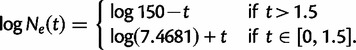
   (1)

In these models, we measure time in expected mutations per site. The genealogy has 30 tips sampled at time . Next, we use a molecular sequence simulator available in BEAST to generate sequence data on the tips of the genealogy. We assume a molecular clock under the HKY85 CTMC model (Hasegawa et al. 1985) with a transition/transversion rate ratio fixed to 4.0. To simulate a data set with unlinked loci, we repeat this process times. We consider data sets with 1, 2, 5, and 10 loci.

We analyze all data sets using the Skygrid model with 29 grid points and a cutoff value of 10. This way, the vector of effective population sizes has length of 30, equal to the number of individuals sampled in the data set. Furthermore, the cutoff value is greater than the root heights of typical genealogies generated by the coalescent under the aforementioned demographic scenarios. This goes toward ensuring that we capture as much of the population trajectory as possible given the data at hand.

Figure 1 illustrates the results of estimating the effective population size trajectories of constant size populations. The bold lines in the plots correspond to posterior medians and 95% Bayesian credibility intervals (BCIs) are shown as gray shaded areas. The dashed lines represent the true population trajectories. The model does a reasonably good job of recovering the true effective population size trajectory. In each plot, the BCIs increase as we move from the present time to the past. This is representative of the fact that, for constant populations, coalescent events become increasingly rare as we move away from the tips of the genealogy and toward the root. In other words, there are typically fewer data points (coalescent events) to inform the estimation near the root of the tree. We also see that the width of the BCI region decreases as more loci are incorporated into the analysis. The shrinkage is most dramatic as we go further back in time where data are scarce. This is due to the fact that increasing the number of loci is a very effective way of providing precious extra information in that time frame, and it illustrates a major advantage of performing a multilocus analysis.

Fig. 1.

Constant population size simulation. We present plots of posterior medians (solid black lines) and 95% BCIs (gray shading) of the effective population size based on data sets with 1, 2, 5, and 10 loci. The true population size trajectories are depicted by dashed lines. Here and in all subsequent plots of effective population sizes, we use the log transformation of the population size axis.

Figure 2 shows the results under the exponential growth demographic model. As is the case with the constant demographic model, including data from additional loci leads to more precise estimation. Note that in each plot, following the trajectory from right to left (from present to past), the posterior median curve is very close to the true effective population size until it reaches a certain point, after which the curve follows a constant trajectory. In each plot, the posterior median becomes constant around the time of the greatest of the root heights of the coalescent trees, which are used to generate the data. For instance, the greatest root height of the trees used to generate the 10-loci data set is 6.07. This flattening occurs because, beyond the greatest root height, the estimated effective population size is primarily informed by the prior rather than the non-existent data. It is important when drawing inferences to take note of the estimated root height to get an idea of where the trajectories are informative and where they are not.

Fig. 2.

Exponential growth simulation. See figure 1 for the legend explanation. The times of divergence between the estimated trajectories in solid black lines and the true trajectories depicted by dashed lines correspond approximately to the greatest root heights of the trees used to generate the data sets and illustrate the importance of the estimated root height in understanding the range over which the plots are informative.

Figure 3 depicts results in the case of populations that undergo a period of exponential growth followed by a period of exponential decline. As in the exponential growth case, the estimated trajectory is constant (and uninformative) during the time frame preceding the greatest root height of the trees used to generate the data. We do not accurately recover the overall trend of the demographic history in the one locus plot. Although it does show a clear period of growth, the decline is rather mild and the time of transition from growth to decline is imprecise and occurs before the actual transition time. However, the remaining plots show that we infer with greater accuracy the transition time and the rates of growth and decline as we incorporate more loci into the analysis. These findings illustrate that important aspects of a population’s demographic history may go undetected in a standard one locus analysis, but that increasing the number of loci can recover them.

Fig. 3.

Simulation for a population that experiences exponential growth followed by a decline. See figure 1 for the legend explanation. As in figure 2, the trajectories are constant (and not informative) for a time range (−10, −7), which precedes the greatest root height of the trees used to generate the data sets. The plots illustrate the improvement in correctly recovering past population trends by incorporating data from additional loci.

Let denote the estimated posterior median effective population size, and and the 2.5 and 97.5% quantiles of the estimated posterior effective population size, respectively. To provide a comparative summary of the performance of our model for data sets with varying numbers of loci, we use the percent error and size, which are defined as follows:

(2)

and

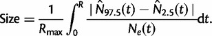(3)

Here, is the maximum of the mean estimated root heights for a given data set and is the root height of the tallest tree used to generate the data set. We use as the upper limit in the integrals because the maximum root height provides an indication of how far back in time the data are informative. Dividing by adjusts the metrics to ensure they provide measures of bias and variance that are not inflated for data sets that are informative for longer time spans.

Our results based on 100 simulated data sets are summarized in table 1. We report relative percent error, which we obtain by dividing the mean percent error of 100 simulated data sets for a given number of loci by the mean percent error of 100 simulated one-locus data sets. We also report the relative size, which is defined analogously.

Table 1.

Improvement of Skygrid Performance with Additional Loci.

Loci	Constant		Exponential		Crash
	Relative		Relative		Relative
	Percent Error	Size	Percent Error	Size	Percent Error	Size
1	1.00	1.00	1.00	1.00	1.00	1.00
2	0.89	0.31	0.75	0.59	0.80	0.68
5	0.69	0.16	0.57	0.38	0.71	0.25
10	0.55	0.13	0.46	0.27	0.69	0.19

Note.—Percent error and size, relative to estimates for one locus data sets, in simulations under the demographic scenarios of constant population size, exponential growth, and exponential growth followed by a crash.

Under all three demographic models, the size and percent error decrease as the number of loci increases. In other words, multilocus data improve estimation in terms of both bias and precision.

To compare the Skygrid with the EBSP, we analyze the same simulated data sets generated for the Skygrid performance analysis using the EBSP. We compare these two models since they are, to our knowledge, the only coalescent-based nonparametric Bayesian models that infer population dynamics from multilocus data. In table 2, we report the relative percent error and size, where we define the relative value of each metric as the mean value over 100 simulations based on EBSP analysis divided by the mean value over 100 simulations based on the Skygrid analysis. The Skygrid almost always outperforms the EBSP by a wide margin in terms of percent error. The EBSP analyses generally have smaller sizes, but in light of the much greater percent error, this extra “precision” is not especially meaningful. Indeed, an investigation of 95% BCI regions and the proportion of the true trajectory that each BCI region covers reveal that the Skygrid outperforms the EBSP 3-fold for the exponentially growing populations and by 6–19% for the constant size populations. The Skygrid thus emerges as a better overall choice in common situations comparable with our simulation set-up.

Table 2.

Performance of EBSP Model Relative to Skygrid.

Loci	Constant		Exponential		Crash
	Relative		Relative		Relative
	Percent Error	Size	Percent Error	Size	Percent Error	Size
1	2.88	0.76	1.23	0.32	0.97	0.20
2	2.94	1.07	1.66	0.50	1.28	0.47
5	2.28	0.93	1.90	0.58	1.26	0.73
10	1.45	0.62	2.41	0.63	1.19	0.76

Note.—Percent error and size based on EBSP analyses, relative to estimates based on Skygrid analyses, in simulations under the demographic scenarios of constant population size, exponential growth, and exponential growth followed by a crash.

Performance and Mixing

In all simulation studies, we simulate MCMC chains of length set to 20 million steps and sub-sample the chain every 1,000 states, after discarding the first 10% as burn-in. To confirm sufficient mixing within the MCMC chain, we examine the effective sample size (ESS) scores of the model parameters and note that all ESS scores for effective population size parameters are more than 1,000.

The inclusion of data from additional loci adds to the complexity of the model and increases the run time necessary to achieve sufficient mixing. To investigate the computational cost of increasing the number of loci in a Skygrid analysis, we examine the ESS scores per unit time for effective population size parameters. We conduct all analyses on a 2.93 GHz Intel Core 2 Duo processor with 4 GB of RAM. ESS per minute for data sets with 1, 2, 5, and 10 loci have respective ranges of 126.9–493.1, 124.8–271.5, 69.2–245.7, and 41.3–137.4 across all ESS parameters. These findings suggest that, while increasing the number of loci in a Skygrid analysis necessitates longer run times, the marginal cost is not especially high. For instance, a 10-fold increase in the number of loci does not require a 10-fold increase to achieve the same ESS. The feasibility of Skygrid analyses of data sets with large numbers of loci is encouraging in light of the increasing availability of multilocus data sets and the improvements they confer upon inference of past population dynamics.

Choice of Cutoff Values and Grid Points

Because it is up to the user to specify the cutoff value and number of grid points , it is natural to wonder how this choice will influence inference. A natural desired feature of the cutoff value is that it be sufficiently greater than the root height of the unobserved coalescent process, thereby allowing the analysis to capture as much information about the population dynamics as the data allow. An initial choice of a cutoff value can be informed by prior knowledge or a time frame of scientific interest. Otherwise, we recommend performing a preliminary analysis and examining the estimated root height to determine the need to possibly adjust the cutoff.

To investigate the sensitivity of the estimated root height to different choices of cutoff values, we consider a 100-taxa data set simulated under an exponential growth demographic model with demographic function . We assume a molecular clock under the HKY85 CTMC model (Hasegawa et al. 1985) with a transition/transversion rate ratio fixed to 4.0. The true root height of the coalescent tree used to generate the data is 27.1. We estimate the root height under our model using cutoff values of . We adjust the number of grid points in each case so that the grid points remain 0.2 units apart. The results are summarized in figure 4. The black dots represent posterior mean root height estimates and are connected by a dotted line, whereas the true root height is marked by a dashed line. The shaded gray rectangles show the coverage of the 95% BCI for each cutoff value.

Fig. 4.

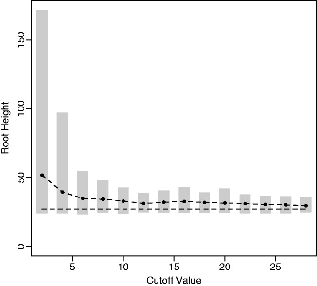
Root height estimate sensitivity. Here, we compare the estimated root height for a simulated exponential growth data set using different cutoff values. The black dots represent posterior mean root height estimates, and the shaded gray rectangles represent the 95% BCIs. The dashed line indicates the true root height of 27.1.

As we see, increasing the cutoff value generally leads to more precise and less biased estimates of the root height. Because low cutoff values force the estimated population size to be constant for the bulk of the demographic history, this illustrates the advantage, when estimating the root height, of using a flexible model that allows the population trajectory to change over time. At the same time, the posterior mean estimated root heights and 95% BCIs using relatively low cutoff values are not especially far off from the estimates found using a cutoff value greater than the true root height. This is convenient because it allows the user to make an informative adjustment of the cutoff value for a subsequent analysis if the current cutoff value turns out to be too low. In our example, low cutoff values lead to overestimates of the root height because constant size populations generally have greater root heights than exponentially growing populations.

In our analysis of cutoff values, we observe another nice feature of the Skygrid, in addition to the generally low root height estimate sensitivity: The choice of cutoff value does not have any notable impact on the trajectory of the estimated effective population size prior to the cutoff value.

With respect to the number of grid points, it is advisable to specify enough points at different times to capture any possible population trends. Our default suggestion is to specify one less grid point than the number of taxa (so that the length of the population size vector will be the same as the number of taxa) and space grid points evenly. This spacing gives us an equal opportunity to detect trends at different times, and the resolution coincides in a rough sense with the amount of available data. However, a major advantage of our model is the ability to set grid points at any desired time. The user has the flexibility, for instance, to concentrate grid points in time intervals in which the data are more informative or in regions in which prior beliefs suggest rapid changes.

Estimation of Time to Most Recent Common Ancestor

It is often of interest to estimate the TMRCA, also known as the root height, from genetic sequence data. Although the Skygrid is in a sense a generalization of the Skyride, the Skyride’s GMRF prior conditions on the genealogy whereas the Skygrid’s does not, and this can affect TMRCA estimation. We wish to compare the performance of the Skygrid, Skyride, and Bayesian Skyline models in estimating the TMRCA from one-locus data sets. We consider the one-locus case because the Skyride is not equipped analyze multilocus data sets. We conduct a series of simulations under three different demographic scenarios. First, a constant population with demographic function , and second, an exponentially growing population with demographic function . The third demographic scenario is a four-epoch piecewise exponential model motivated by the Beringian bison data set discussed later.

To analyze a data set of 152 mtDNA control region sequences from ancient bison in Beringia (Siberia, Alaska, and north-western Canada) and central North America, Shapiro et al. (2004) implement a coalescent-based two-epoch parametric demographic model in BEAST. The model is characterized by two phases of exponential growth at different rates, and a transition time between the phases. Their analysis suggests an initial phase of exponential growth followed by a period of exponential decline, with a transition time approximately 32–43 ka BP (where 1 ka BP is 1,000 years before present). The estimated TMRCA has a posterior mean of 136 ka BP with a 95% BCI of (111, 164 ka BP).

We analyze the same data using the Skyride as well as our Skygrid model (with 150 grid points and a cutoff of 150 ka BP). Both analyses suggest a period of sustained population growth, peaking at about 35–45 ka BP, followed by a period of decline bottoming out approximately 10 ka BP, and then a postbottleneck recovery. The postbottleneck recovery, which is not identified by the two-epoch parametric model, is also observed in a nonparametric analysis by Drummond et al. (2005) using the Bayesian Skyline. Although all of the nonparametric analyses uncover similar demographic histories, the same cannot be said for estimating the TMRCA. The Skyride gives us a posterior mean TMRCA of 101.45 ka BP with a 95% BCI of (87.12, 117.5 ka BP), the Bayesian Skyline gives us a posterior mean TMRCA of 133.56 ka BP with a 95% BCI of (103.86, 167.63 ka BP), and the Skygrid yields a posterior mean of 130.39 ka BP with a 95% BCI of (99.99, 159.54 ka BP).

The Skygrid and Bayesian Skyline estimates are similar to those of Shapiro et al. (2004), whereas the Skyride analysis paints a substantially different picture. The Skyride results do not agree with the North American fossil record; bison are known to have been present in Alaska during the last interglacial interval (150–100 ka BP). To further investigate which estimates are closer to the truth, we test the Skygrid, Bayesian Skyline, and Skyride on simulated data sets that are similar to the bison data set. We generate the data sets using evolutionary parameter values similar to the estimated values from the bison data set along with a four-epoch demographic model (which we refer to as the “Ancient DNA” model) that grows and declines exponentially at approximately the same times and rates as the estimated trajectory using the Skygrid model on the bison data.

For each of the three demographic scenarios, we simulate 100 one-locus genetic sequence data sets and estimate the root heights using the three different models. To provide a comparative summary of the performance, we define the percent error as follows:

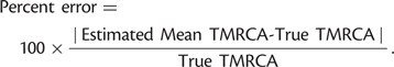(4)

Also, we define the size of each estimate as the length of the 95% BCI. Finally, we monitor the percentage of BCIs that contain the true root height as a measure of frequentist coverage, a useful property for inference tools that will be applied to many independent data sources. Ideally, estimated coverage should approach its nominal level; 0.95 in this case.

The simulation results are presented in table 3. The three different models exhibit similar performance in the constant and exponential growth demographic scenarios. The Skygrid performs slightly better than the other two models in the case of exponentially growing populations. For the constant population simulations, each of the three performance metrics identifies a different model as the best, and none of the models dramatically outperforms the others in any way. In the ancient DNA demographic scenario, the Skygrid outperforms both models. The contrast with the Skyride in terms of relative error and frequentist coverage of the true root height is especially dramatic. For each of the three demographic situations, the Skygrid model performs as good or better than the Skyride and Bayesian Skyline. Our simulation studies thus offer support for the Skygrid as the best of the three models for estimating the TMRCA from populations with a variety of demographic histories.

Table 3.

Estimation of Time to Most Recent Common Ancestor.

Model	Demographic	Percent Error	Size	Frequentist Coverage
Skyride	Constant	3.99	0.77	89
Skyline	Constant	3.69	0.79	94
Skygrid	Constant	3.66	0.79	92
Skyride	Exponential	0.99	0.26	92
Skyline	Exponential	1.02	0.26	91
Skygrid	Exponential	0.99	0.26	94
Skyride	Beringian bison	69.79	24,621.74	1
Skyline	Beringian bison	9.90	77,742.94	96
Skygrid	Beringian bison	9.29	74,634.97	96

Note.—Size is measured in years for Ancient DNA demographic and in substitutions per site for other demographic models. Here, Skyline refers to the Bayesian Skyline.

Population History of HIV-1 CRF02_AG Clade in Cameroon

Circulating recombinant forms (CRFs) are genomes that result from recombination of two or more different HIV-1 subtypes and that have been found in at least three epidemiologically unrelated individuals. CRF02_AG is globally responsible for 7.7% of HIV infections (Hemelaar et al. 2011), but HIV/AIDS surveillance studies indicate that it accounts for approximately 60% of infections in Cameroon (Brennan et al. 2008).

Faria et al. (2012) investigate the population dynamics of the CRF02_AG lineage through a multilocus alignment of 336 gag (HXB2: 1255–1682), pol (HXB2: 4228–5093), and env (HXB2: 7890–8266) CRF02_AG gene sequences sampled between 1996 and 2004 from blood donors from Yaounde and Douala (Brennan et al. 2008). Given the high rate of recombination in HIV, it is common to assume these three genes are unlinked. Following this assumption, Faria et al. (2012) use BEAST to conduct a multilocus analysis employing a parametric piecewise constant-logistic demographic tree prior model. Their analysis suggests a period of exponential growth of the viral effective population size until the mid 1990s at which point the growth levels off. The estimated origins of the most recent common ancestors for the , , and sequences are 1967.6 (95% BCI: 1962.4, 1972.4), 1967.6 (95% BCI: 1962.5, 1972.5), and 1968.1 (95% BCI: 1962.8, 1972.8), respectively.

We perform a multilocus Skygrid analysis of the same data with 50 grid points and a cutoff value of 50 years. Figure 5 depicts the resulting estimated posterior median log effective population size along with estimated HIV prevalence counts in Cameroon from 1990 to 2004 (UNAIDS/WHO 2008). Like the parametric multilocus analysis, the Skygrid analysis points to a period of exponential growth in effective population size from 10 to 30 years prior to the most recent sampling time. It also yields similar results regarding the origin of the HIV-1 CRF02_AG clade. TMRCAs for the , , and sequences have estimates of 1965.2 (95% BCI: 1959.6, 1970.1), 1967.3 (95% BCI: 1962.8, 1971.3), and 1969.3 (95% BCI: 1963.1, 1974.1), respectively. However, in contrast to the parametric multilocus analysis, the Skygrid analysis suggests a dip in effective population size over the 5 years prior to the most recent sampling time. This finding is supported by the drop in HIV-1 prevalence in Cameroon from 2000 to 2004, but is not detected by the parametric multilocus analysis due to the a priori constraints on the shape of the effective population size trajectory imposed by the logistic-constant demographic model prior. It should be noted that the CRF02_AG population in Cameroon will have some gene flow with the worldwide population of CRF02_AG, and this is not modeled in our Skygrid analysis or the earlier parametric analysis. This may account for some of the discordance between the inferred population sizes and the Cameroon prevalence counts.

Fig. 5.

Population history of HIV-1 CRF02_AG clade in Cameroon. The curve represents the estimated median log effective population size estimated from a multilocus alignment of 336 , , and sequences sampled between 1996 and 2004. The bars represent estimated HIV prevalence counts in Cameroon.

Prior Sensitivity

The GMRF smoothing prior we place on the vector of log effective population sizes informs our model about the smoothness of the trajectory. The precision parameter governs the level of smoothness. There is usually little a priori knowledge regarding the smoothness of the effective population size trajectory, and in all of our examples we assign a relatively uninformative gamma prior. To investigate the sensitivity of our results to different hyperprior parameter values, we follow the suggestion of Minin et al. (2008) and analyze the Beringian bison data set with five different values of : 0.001, 0.002, 0.005, 0.01, and 0.1, leaving unchanged. These choices correspond to increasing prior means of 1, 2, 5, 10, and 100, respectively. Table 4 presents the estimated posterior means and 95% BCIs of . The results demonstrate that the posterior distribution of is robust to alterations of the hyperprior parameter . Moreover, they suggest that the data contain sufficient information to estimate .

Table 4.

GMRF Precision Sensitivity to Prior.

Prior Mean	Posterior
	Mean	95% BCI
1	5.27	0.58–11.82
2	5.37	0.63–11.60
5	5.19	0.50–11.42
10	5.12	0.59–11.68
100	5.40	0.76–12.50

Note.—Posterior estimates of precision parameter corresponding to different choices of prior mean. We use the Beringian bison data.

Discussion

The Skygrid is a powerful, flexible new model for nonparametric coalescent-based inference of past population dynamics from molecular sequence data. It incorporates a GMRF smoothing scheme similar to that of the Skyride, and provides smooth and realistic estimates of demographic histories. Like the Skyride, the Skygrid model does a fairly good job of recovering essential features of simulated data based on standard parametric coalescent models.

However, the Skygrid is an improvement over the Skyride in a number of important ways. It allows for estimation based on multilocus data, yields improved TMRCA estimation, and it gives the user additional flexibility.

Molecular sequence data sets from effectively unlinked loci are becoming increasingly common thanks to lower DNA sequencing costs. Accordingly, there is a need for multilocus statistical approaches to reap the benefits. The Skygrid provides estimates of effective population size trajectories based on samples from several different genetic loci with the same demographic histories. One of the primary difficulties in coalescent-based approaches is that most of the coalescent events in the reconstructed genealogy usually occur in a short time span. During the long periods of time in which few coalescent events occur, there are not much data to infer the population dynamics. This problem is mitigated to a certain extent by increasing the sample size, but the additional coalescent events tend to occur in a small stretch of time. Increasing the number of loci more effectively provides extra information during the long stretches of time with few coalescent events (Felsenstein 2006). We demonstrate through a series of simulations that incorporating data from additional loci yields more precise and less biased estimates of past population dynamics. We also note that multilocus data are especially helpful in improving estimation during time periods for which single locus data are not very informative.

We compare our Skygrid model with existing multilocus approaches. As seen in the analysis of HIV-1 CRF02_AG gene sequences sampled from Cameroon, our nonparametric approach enables detection of a decline in the effective population size that is supported by HIV-1 prevalence data. This aspect of the population history went unnoticed in a multilocus analysis employing a parametric constant-logistic demographic tree model prior. The only other currently available nonparametric Bayesian model that enables estimation of past population dynamics from multilocus data is the EBSP. We analyze simulated data sets with the Skygrid and the EBSP and find that the Skygrid performs more favorably.

Bayesian nonparametric models for inference of population histories typically estimate genealogies and mutation parameters jointly along with effective population size trajectories. The different priors placed on the effective population size that distinguish these models can affect estimation of quantities other than the population history, notably the TMRCA. In simulation studies to explore TMRCA estimation, we consider data sets generated from a variety of different parametric demographic scenarios. These include typical constant and exponential growth demographic models, as well as a more complicated piecewise-exponential model motivated by a data set of ancient DNA from Beringian bison. Considered along with the Skyride and Bayesian Skyline models, the Skygrid emerges as the best overall choice for TMRCA estimation in these examples.

Unlike the Skyride, the Skygrid allows the user to specify the spacing of points where the effective population size of the estimated trajectory can change. This flexibility can be especially convenient for future extensions of the model, which incorporate covariate values which must, necessarily, be measured at fixed times. We anticipate that such extensions will lead to further improvement in estimation of the effective population size over time and, for instance, enable statistical testing of environmental effects on population histories.

Materials and Methods

Coalescent Background

Coalescent theory was first developed by Kingman (1982). Considering a random population sample of individuals arising from a classic Fisher–Wright population model of constant size , Kingman developed a stochastic process called the coalescent to generate genealogies relating the sample. The process begins at a sampling time and proceeds backward in time as increases, successively merging lineages until all lineages have merged. The merging of lineages is called a coalescent event and there are coalescent events in all. Let denote the time of the coalescent event for and denote the sampling time. Then for the waiting time is exponentially distributed with rate .

Griffiths and Tavaré (1994) provide a generalization of the coalescent that allows for the effective population size to change over time. Here, is the effective population size at the sampling time, and is the effective population size time units before the sampling time. In this case, the waiting time is given by the conditional density

(5)

Taking the product of such densities yields the joint density of intercoalescent waiting times, and this fact can be exploited to obtain the probability of observing a particular genealogy given a demographic function. Here, we consider a piecewise constant demographic function that changes values at pre-specified times.

Piecewise Constant Demographic Model

We start by assuming there are known genealogies. Let be a vector of genealogies representing the ancestry of populations with the same effective population size , where the time increases into the past. We assume a priori that the genealogies are independent given . This assumption implies that the genealogies are unlinked which commonly occurs when researchers select loci from whole genome sequences or when recombination is very likely, such as between genes in retroviruses. Let denote the number of points we desire for a fixed-time grid, and let be a positive real cutoff value. Then the temporal grid points are . Here, we assume the grid points are equally spaced, but the model easily extends to arbitrarily spaced grid points.

We estimate the effective population size as a piecewise constant function that changes values only at grid points. The cutoff value is the time furthest back into the past at which the effective population size changes. Notice that for all times further into the past than the cutoff value, . Let be the vector of effective population sizes. Here, for , where it is understood that . Also, for .

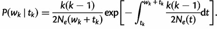
To construct the likelihood of genealogy , let be the most recent sampling time and the TMRCA (also referred to as the root height of genealogy ). Let denote the smallest grid point greater than at least one sampling time in the genealogy, and the greatest grid point less than at least one coalescent time. Let , , , and . For each , we let , , denote the ordered times of the grid points and sampling and coalescent events in the interval. With each , we associate an indicator which takes a value of 1 in the case of a coalescent event and 0 otherwise. Also, let denote the number of lineages present in the genealogy in the interval . 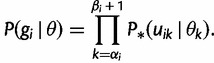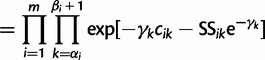Following Griffiths and Tavaré (1994), the likelihood of observing an interval is

(6)

for .

Let denote except with any TMRCA factors of the form replaced by ; this is for the purpose of computing the probability of a genealogy, where the specific branches of a tree which coalesce matters. Then

(7)

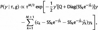
We introduce some notation that will facilitate the derivation of the Gaussian approximation in the next section. If denotes the number of coalescent events, which occur during interval , we can write

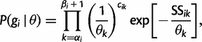(8)

where the are appropriate constants. Rewriting this expression in terms of , we arrive at

(9)

Assuming conditional independence of genealogies, the likelihood of the vector of genealogies is

(10)

(11)

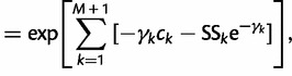(12)

where and 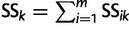; here, if .

To incorporate the prior assumption that effective population size changes continuously over time, we put the following GMRF prior on :

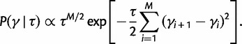(13)

This prior posits that differences between adjacent elements of are normally distributed with mean and estimable precision , drawing motivation from a Brownian diffusion process. Let be a square matrix of dimension with entries for and , for and for . Then, we can write

(14)

Finally, we assign a gamma prior:

(15)

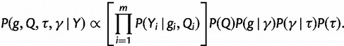
This yields the following posterior distribution:

(16)

It should be noted that the GMRF prior does not inform the overall level of the estimated effective population size, just the smoothness of the trajectory. The degree of smoothness is determined by the precision . Researchers typically do not have any prior knowledge about the smoothness of the effective population size trajectory, and in such cases it is appropriate to use relatively uninformative priors. Accordingly, we choose in our examples, giving a prior mean of 1 and variance of 1,000.

Markov Chain Monte Carlo Sampling Scheme

We use a block-updating Markov chain Monte Carlo sampling scheme (Knorr-Held and Rue 2002) to approximate the posterior given in Equation (16). First, consider the full conditional density

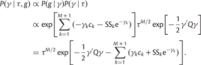(17)

Let 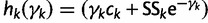. We can approximate each term by a second-order Taylor expansion about, say, :

(18)

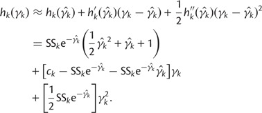
This yields the following second-order Gaussian approximation:

(19)

where is a diagonal matrix.

Now suppose we have current parameter values . First, we generate a candidate value for the precision, , where is drawn from a symmetric proposal distribution with density defined on . The tuning constant controls the distance between the proposed and current values of the precision. Next, conditional on , we propose a new state using the aforementioned Gaussian approximation to the full conditional density . In the Gaussian approximation, we center the Taylor expansion about a point obtained iteratively by the Newton–Raphson method:

(20)

with . Here

(21)

and

(22)

and

(23)

Finally, the candidate state is accepted or rejected in a Metropolis–Hastings step.

Incorporation of Genealogical Uncertainty

In our development thus far, we have assumed the genealogies are known and fixed. However, in reality we observe sequence data rather than genealogies. We can think of the aligned sequence data as arising from continuous-time Markov chain (CTMC) models for molecular character substitution that act along the hidden genealogies. Each CTMC depends on a vector of mutational parameters , that include, for example, an overall rate multiplier, relative exchange rates among characters and across-site variation specifications. We let . We then jointly estimate the genealogies, mutational parameters, precision, and vector of effective population sizes through their posterior distribution

(24)

Here, the coalescent acts as a prior for the genealogies, and we assume that and are a priori independent of each other. Hierarchical models are however available to share information about among loci without strictly enforcing that they follow the same evolutionary process (Edo-Matas et al. 2011).

We achieve joint estimation by integrating the block-updating MCMC scheme for the fixed-trees case into the software package BEAST (Drummond et al. 2012). We plan to provide a user-friendly interface to this joint model in the next public release of BEAUti (Drummond et al. 2012), a graphical user interface application for generating BEAST model and data description files. In the meantime, we welcome users to exploit this multilocus model in the development branch of the BEAST source code repository (http://beast-mcmc.googlecode.com/svn/trunk). Examples of XML specification for the model are available at http://beast.bio.ed.ac.uk.

References

- Baele G, Lemey P, Bedford T, Rambaut A, Suchard MA, Alekseyenko AV. Improving the accuracy of demographic and molecular clock model comparison while accommodating phylogenetic uncertainty. Mol Biol Evol. 2012;29:2157–2167. doi: 10.1093/molbev/mss084. [DOI] [PMC free article] [PubMed] [Google Scholar]
- Brennan C, Bodelle P, Coffey R, et al. (20 co-authors) The prevalence of diverse HIV-1 strains was stable in Cameroonian blood donors from 1996 to 2004. J Acquir Immune Defic Snyrd. 2008;49:432–439. doi: 10.1097/QAI.0b013e31818a6561. [DOI] [PubMed] [Google Scholar]
- Campos P, Willerslev E, Sher A, et al. (20 co-authors) Ancient DNA analyses exclude humans as the driving force behind late plestocene musk ox (Ovibos moschatus) population dynamics. Proc Natl Acad Sci U S A. 2010;107:5675–5680. doi: 10.1073/pnas.0907189107. [DOI] [PMC free article] [PubMed] [Google Scholar]
- Donnelly P, Tavaré S. Coalescents and genealogical structure under neutrality. Annu Rev Genet. 1995;29:401–421. doi: 10.1146/annurev.ge.29.120195.002153. [DOI] [PubMed] [Google Scholar]
- Drummond A, Nicholls G, Rodrigo A, Solomon W. Estimating mutation parameters, population history, and genealogy simultaneously from temporally spaced sequence data. Genetics. 2002;161:1307–1320. doi: 10.1093/genetics/161.3.1307. [DOI] [PMC free article] [PubMed] [Google Scholar]
- Drummond A, Rambaut A, Shapiro B, Pybus O. Bayesian coalescent inference of past population dynamics from molecular sequences. Mol Biol Evol. 2005;22:1185–1192. doi: 10.1093/molbev/msi103. [DOI] [PubMed] [Google Scholar]
- Drummond A, Suchard M, Xie D, Rambaut A. Bayesian phylogenetics with BEAUti and the BEAST 1.7. Mol Biol Evol. 2012;29:1969–1973. doi: 10.1093/molbev/mss075. [DOI] [PMC free article] [PubMed] [Google Scholar]
- Edo-Matas D, Lemey P, Tom JA, Serna-Bolea C, van den Blink AE, van’t Wout AB, Schuitemaker H, Suchard MA. Impact of ccr5delta32 host genetic background and disease progression on HIV-1 intrahost evolutionary processes: efficient hypothesis testing through hierarchical phylogenetic models. Mol Biol Evol. 2011;28:1605–1616. doi: 10.1093/molbev/msq326. [DOI] [PMC free article] [PubMed] [Google Scholar]
- Faria N, Suchard M, Abecasis A, Sousa J, Ndembi N, Bonfim I, Camacho R, Vandamme A, Lemey P. Phylodynamics of the HIV-1 CRF02_AG clade in Cameroon. Infect Genet Evol. 2012;12:453–460. doi: 10.1016/j.meegid.2011.04.028. [DOI] [PMC free article] [PubMed] [Google Scholar]
- Felsenstein J. Accuracy of coalescent likelihood estimates: do we need more sites, more sequences, or more loci? Mol Biol Evol. 2006;23:691–700. doi: 10.1093/molbev/msj079. [DOI] [PubMed] [Google Scholar]
- Griffiths R, Tavaré S. Sampling theory for neutral alleles in a varying environment. Philos Trans R Soc London B: Biol Sci. 1994;344:403–410. doi: 10.1098/rstb.1994.0079. [DOI] [PubMed] [Google Scholar]
- Hasegawa M, Kishino H, Yano T. Dating the human-ape splitting by a molecular clock of mitochondrial DNA. J Mol Evol. 1985;22:160–174. doi: 10.1007/BF02101694. [DOI] [PubMed] [Google Scholar]
- Hein J, Schierup M, Wiuf C. New York: Oxford University Press; 2005. Gene genealogies, variation, and evolution. [Google Scholar]
- Heled J, Drummond A. Bayesian inference of population size history from multiple loci. BMC Evol Biol. 2008;8:289. doi: 10.1186/1471-2148-8-289. [DOI] [PMC free article] [PubMed] [Google Scholar]
- Hemelaar J, Gouws E, Ghys PD, Osmanov S, WHO-UNAIDS Network for HIV Isolation and Characterisation Global trends in molecular epidemiology of HIV-1 during 2000–2007. AIDS. 2011;25:679–689. doi: 10.1097/QAD.0b013e328342ff93. [DOI] [PMC free article] [PubMed] [Google Scholar]
- Kingman J. On the genealogy of large populations. J Appl Prob. 1982;19:27–43. [Google Scholar]
- Knorr-Held L, Rue H. On block updating in Markov random field models for desease mapping. Scand J Statist. 2002;29:597–614. [Google Scholar]
- Kuhner M, Yamato J, Felsenstein J. Maximum likelihood estimation of population growth rates based on the coalescent. Genetics. 1998;149:429–434. doi: 10.1093/genetics/149.1.429. [DOI] [PMC free article] [PubMed] [Google Scholar]
- Minin V, Bloomquist E, Suchard M. Smooth skyride through a rough skyline: Bayesian coalescent based inference of population dynamics. Mol Biol Evol. 2008;25:1459–1471. doi: 10.1093/molbev/msn090. [DOI] [PMC free article] [PubMed] [Google Scholar]
- Opgen-Rhein R, Fahrmeir L, Strimmer K. Inference of demographic history from genealogical trees using reversible jump Markov chain Monte Carlo. BMC Evol Biol. 2005;5:6. doi: 10.1186/1471-2148-5-6. [DOI] [PMC free article] [PubMed] [Google Scholar]
- Pybus O, Rambaut A, Harvey P. An integrated framework for the inference of viral population history from reconstructed genealogies. Genetics. 2000;155:1429–1437. doi: 10.1093/genetics/155.3.1429. [DOI] [PMC free article] [PubMed] [Google Scholar]
- Rambaut A, Pybus O, Nelson M, Viboud C, Taubenberger J, Holmes E. The genomic and epidemiological dynamics of human influenza A virus. Nature. 2008;453:615–619. doi: 10.1038/nature06945. [DOI] [PMC free article] [PubMed] [Google Scholar]
- Rodrigo A, Felsenstein J. Baltimore (MD): Johns Hopkins University Press; 1999. The evolution of HIV. Coalescent approaches to HIV population genetics. [Google Scholar]
- Shapiro B, Drummond A, Rambaut A, et al. (co-authors) Rise and fall of the Beringian steppe bison. Science. 2004;306:1561–1565. doi: 10.1126/science.1101074. [DOI] [PubMed] [Google Scholar]
- Strimmer K, Pybus O. Exploring the demographic history of DNA sequences using the generalized skyline plot. Mol Biol Evol. 2001;18:2298–2305. doi: 10.1093/oxfordjournals.molbev.a003776. [DOI] [PubMed] [Google Scholar]
- UNAIDS/WHO. Geneva (Switzerland): UNAIDS/WHO; 2008. UNAIDS/WHO epidemiological fact sheets on HIV and AIDS, 2008 update. [Google Scholar]