Accurate measurements of dynamics and reproducibility in small genetic networks

Abstract

Quantification of gene expression has become a central tool for understanding genetic networks. In many systems, the only viable way to measure protein levels is by immunofluorescence, which is notorious for its limited accuracy. Using the early Drosophila embryo as an example, we show that careful identification and control of experimental error allows for highly accurate gene expression measurements. We generated antibodies in different host species, allowing for simultaneous staining of four Drosophila gap genes in individual embryos. Careful error analysis of hundreds of expression profiles reveals that less than ∼20% of the observed embryo-to-embryo fluctuations stem from experimental error. These measurements make it possible to extract not only very accurate mean gene expression profiles but also their naturally occurring fluctuations of biological origin and corresponding cross-correlations. We use this analysis to extract gap gene profile dynamics with ∼1 min accuracy. The combination of these new measurements and analysis techniques reveals a twofold increase in profile reproducibility owing to a collective network dynamics that relays positional accuracy from the maternal gradients to the pair-rule genes.

Introduction

The final macroscopic outcome of developmental processes in multicellular organisms results in structures that are remarkably similar between individuals of a given species (Thompson, 1917; Held, 1991). In insects, this has long been observed for the determination of sensory bristles of the adult (Wigglesworth, 1940; Richelle and Ghysen, 1979; Whittle, 1998). In fly embryos, in particular, the segmentally repeated denticle pattern of the ventral epidermis is homologous from one region to the next and identical from one individual to the next (Alexandre et al, 1999; Hatini et al, 2000; Jones and Bejsovec, 2005). The earliest macroscopic manifestation of reproducible pattern in the fly embryo can be identified as the formation of the cephalic furrow (Namba et al, 1997), which forms only 3 h after the egg is fertilized. The swift appearance of enduring reproducible features suggests that the observed similarities may have their origins at the molecular level in the reproducible spatial patterns of morphogen concentrations in the early embryo (Lawrence, 1992, Arias and Hayward, 2006; Kerszberg and Wolpert, 2007; Lander, 2007; Gregor et al, 2007a).

Uncovering the origin of precise and reproducible structures in biological processes is a fundamentally quantitative question, the answer to which can be one of two very distinct concepts (Schrödinger, 1944). In one view, each step in the process is noisy and variable, and noise reduction only occurs through integration of many elements or collectively within the whole network of elements. In the other view, each step in the process has been tuned to enhance its reliability, at times maybe even down to the limits set by basic physical principles (Gregor et al, 2007a). Can the precise and reproducible features observed in the patterning system be sufficient to account for the precision observed in morphology? Focusing on these quantitative features of the network will ultimately lead to our understanding of which network properties are truly reliable, which ones are variable, how they relate to network architecture, and how they respond to environmental and genetic variation.

Studies of the emergence of reproducible patterns during embryogenesis typically utilize genetic tools to disrupt entire nodes of the regulatory network (e.g., Driever et al, 1989; Hülskamp et al, 1990; Kraut and Levine, 1991; Capovilla et al, 1992; Struhl et al, 1992; Rivera-Pomar et al, 1995. See Sánchez and Thieffry, 2001 for a full review). The subsequent response of the system is then used to infer interactions between the remaining network components. As a complementary approach, precise measurements in an intact, wild-type system can reveal the quantitative relationships within the network in an unperturbed, natural state (Mjolsness et al, 1991; Reinitz and Sharp, 1995; Reinitz et al, 1998; Jaeger et al, 2004b; Crombach et al, 2012). It is challenging to perform experiments that take advantage of the latter approach as it requires extreme care to minimize sources of experimental error that allow for the data to be accurately quantified. Nevertheless, such measurements are essential both for mathematical modeling of gene interactions and for understanding increasingly complex development systems.

To fully understand the source and maintenance of developmental reproducibility, and the level of reproducibility that is actually relevant to biological processes (i.e., the level of variation that is tolerated by the system while still maintaining function), a number of conceptual and technical challenges need to be overcome (Kudoh et al, 2001; Myasnikova et al, 2001; Visel et al, 2004; Tassy et al, 2006; Lein et al, 2007; Tomancak et al, 2007; Fakhouri et al, 2010). Conceptually, we are seeking to uncover novel quantitative traits in developmental regulatory networks, such as the time dependence of simultaneously measured expression levels, and their position-dependent variances and cross-correlations across populations of comparable embryos. Technically, such quantities cannot be determined precisely in the presence of systematic experimental bias or measurement error.

Quantitative data in this context is largely based on immunofluorescence staining (Ay et al, 2008; Fowlkes et al, 2008; Surkova et al, 2008; Pisarev et al, 2009), a technique that is restricted to fixed tissue and induces systematic errors inherent to the experimental procedure. These fluctuations are thought to have only a minor effect on the measurement of the mean expression profiles (Myasnikova et al, 2009). However, if one is interested in quantifying the variations that naturally arise from embryo-to-embryo, such experimental error will distort the signal. Moreover, using fixed tissues makes it difficult to reconstruct gene expression dynamics (Myasnikova et al, 2001). Finally, because the number of simultaneously stainable genes is limited, comparisons of different genes at any given time point are restricted.

Here, we address these issues of the fixed-tissue approach in the context of the gap gene network in the early fly embryo. We show that precise measurements in conjunction with proper quantification of experimental error enable (i) simultaneous spatial and temporal tracking of gene expression levels; (ii) quantification of reproducibility at an unprecedented level of precision; and (iii) hitherto unmatched access to questions about the interactions between the genes.

In embryos of the fruit fly Drosophila melanogaster, the earliest sign of a reproducible pattern is the gradient of bicoid (Bcd), the primary anterior determinant of patterning along the major body axis (Driever and Nüsslein-Volhard, 1988; Crauk and Dostatni, 2005; He et al, 2008; de Lachapelle and Bergmann, 2010), and which is established by maternally deposited mRNA at the anterior pole of the egg (Ephrussi and St Johnston, 2004). In its main region of activity between 10 and 60% egg length (EL; where 0% corresponds to the anterior pole of the egg), the gradient has been shown to be reproducible to ∼10% in Bcd concentration across different embryos, which translates into a positional accuracy of 1–2% EL (Gregor et al, 2007a). Bcd, acting as a transcription factor, triggers the expression of Hunchback (Hb) and other downstream zygotic genes such as the gap, pair-rule, and segment polarity genes. These genes interact with each other in a complex network (Nüsslein-Volhard and Wieschaus, 1980; Akam, 1987; Ingham, 1988; Hülskamp et al, 1990; Kraut and Levine, 1991; Papatsenko, 2009; Jaeger, 2011), resulting 3 h after fertilization in the formation of precise patterns in which neighboring cells have readily distinguishable levels of gene expression (Gergen and Wieschaus, 1986), and which are reproducible from embryo-to-embryo (Houchmandzadeh et al, 2002; Gregor et al, 2007a). In order to understand the strategies that nature uses to make embryonic development so reproducible, it is crucial to precisely record the variations in gene expression levels across embryos over time (Gregor et al, 2007b). In particular, what is the final gene expression level reproducibility at the time of gastrulation and how does it compare with the initial reproducibility of the Bcd gradient (Gregor et al, 2007a)? What is the response of the gap gene network to the Bcd input (Ochoa-Espinosa et al, 2009); and how is reproducibility transmitted from Bcd to the pair-rule genes (Houchmandzadeh et al, 2002; Gregor et al, 2007a)?

In this paper, we present a set of tools and a number of careful control measurements that clearly demonstrate to what extent antibody stainings can be used for quantitative analysis. First, we developed a new set of antibodies for the four major gap genes, Hb, Krüppel (Kr), Giant (Gt), and Knirps (Kni), which allows us to stain individual embryos with all four antibodies at once, and hence to preserve temporal correlations between these genes. Second, we measure the developmental time point of embryos at the instant of fixation with a precision of 1–2 min using the membrane furrow invagination as a calibrator. Third, we identify eight sources of experimental measurement error, and show that the combined sum of these errors for any gene is <20% of the total variance in our data set, leaving over 80% of the variance available for biological interpretation.

To demonstrate the potential of this approach, we connect the dynamics and reproducibility of the gap gene expression patterns with the positional precision of various position markers. Specifically, we compute the positional error of 20 individual position markers (such as boundary positions and the positions of the peak concentrations of all four major gap genes) in a set of 163 embryos. We show that at any time during nuclear cycle (n.c.) 14 all markers of all genes are reproducible below one internuclear distance. We further see a dynamic increase of this reproducibility (averaged over all markers) from one internuclear distance at the beginning of n.c. 14 to half an internuclear distance 40–45 min later. This reduction coincides with an overall zenith of the gap gene network, when all gap genes simultaneously peak in their maximum concentration as well as their maximum boundary slopes. These results lead us to postulate that along the central 80% of the embryo collective network dynamics increase positional accuracy twofold from the level of reproducibility inherent to the Bcd gradient to that observed in the pair-rule genes.

Results

Quadruple antibody stainings in individual embryos

When labeling different proteins with fluorescent probes in the same tissue, there are two main limitations. The first limitation is biochemical: antibodies are raised in specific host animals, so each antibody used to label a given tissue has to be made in a different animal, of which only a limited number exist commercially. The second limitation is optical: secondary antibodies are conjugated with fluorophores whose absorption and emission spectra can significantly overlap, which leads to crosstalk between the different optical channels, making quantification of co-labeled proteins challenging. Some attempts have been made in the past to try to overcome those limitations (direct labeling (Kosman et al, 2004), use of quantum dots as fluorescent probes (Choi et al, 2009), spectral imaging (Dickinson et al, 2001), and blind source separation (Neher et al, 2009)) but to our knowledge there has been no attempt to use the classic immunofluorescence staining protocol to simultaneously quantify more than three co-labeled proteins with high precision.

To overcome the biochemical limitation, we developed a new set of primary polyclonal antibodies against three of the four main gap genes (Kosman et al, 1998). All antibodies were raised in a different host species (rat anti-Kni, guinea pig anti-Gt, and mouse anti-Hb), allowing us to use them in combination with a rabbit anti-Kr antibody (gift of C Rushlow) to simultaneously stain all four major gap genes in the same embryo without the risk of cross-reactivity between reagents. To ensure that our immunofluorescence protocol would potentially be suitable for gene expression profile quantification with these new antibodies, we verified their linearity by comparing immunofluorescence intensities and protein concentrations nucleus per nucleus in individual embryos (see Materials and methods and Supplementary Figure 1).

To overcome the optical limitation, we chose fluorophores that maximized the span of the employable laser excitation wavelengths to limit simultaneous excitation of multiple fluorophores, and we adjusted the bandwidths of the emission channels in order to minimize simultaneous emission from multiple fluorophores in the same imaging channel (see Figure 1A). We used this setup to stain and image a batch of 163 Drosophila embryos at the blastoderm stage. A typical embryo imaged in all four channels is depicted in Figure 1B. Typical intensity profiles extracted from these images are shown in Figure 1C, and cross-talk between channels is quantified in Figure 1D. This approach allows us to measure expression profiles of all four major gap genes simultaneously in individual embryos, an indispensable requirement to measure natural fluctuations and cross-correlations of profile variabilities across genes and to guarantee temporal order and correlations for these measurements.

Figure 1.

Simultaneous immunostaining of the four main gap genes. (A) Spectral imaging settings for simultaneous measurements of four fluorescent dyes. Absorption (dashed lines) and emission (solid lines) spectra of the dyes used for four simultaneous immunostainings; laser excitation wavelengths (black arrows) and bandwidths of the emission filters for each detection channel (light color patches) are indicated. (B) Optical sections through the midsagittal plane of a single Drosophila embryo with co-immunofuorescence staining against the four gap genes Kni (green), Kr (yellow), Gt (orange), and Hb (red); scalebar 100 μm. (C) Raw intensity profiles (dorsal side) of 23 selected embryos (light colors); embryo depicted above is highlighted in darker color (anterior pole at x/L=0; posterior pole at x/L=1). (D) Quantification of spectral crosstalk and fluorophore bleed-through. For each channel, the average intensity profile I of 10 embryos immunofluorescently labeled with three antibodies lacking the specific antibody corresponding to that optical channel is shown in gray. Black dashed line shows a cross-talk estimate using a reconstruction algorithm (see Materials and methods). Average profiles from B are shown in color.

Developmental time measurements in fixed embryos

The Drosophila gap genes are endogenously transcribed for a time span of 1–2 h, peaking roughly 2.5 h after the onset of embryonic development. During this entire time, gene expression patterns change significantly, making the determination of each individual embryo’s age with high fidelity a crucial prerequisite for any quantitative purpose such as assessing the profiles’ reproducibility. Fortunately, in the Drosophila embryo the 1-h time window before gastrulation (i.e., n.c. 14) can be temporally staged in a very precise way. During this time, cell membranes form in an apical–basal direction across the entire embryo surface, and we can use the progression of this cellularization process (by measuring the depth δ_FC of the membrane furrow canal (FC)) as a ‘clock’ to estimate the age of the embryo (see Figure 2A and Lecuit et al, 2002).

Figure 2.

Staging of gene expression profiles in fixed embryos with minute precision. (A) Depth of FC (δ_FC) during blastoderm cellularization measured along the dorsal side of a live-imaged wild-type embryo during n.c. 14. Dashed line corresponds to our estimate of mitosis 13. Inset shows a bright field microscopy image of a fraction (40–50%EL) of the dorsal side of the embryo at a time point indicated by red dot; scale bar 10 μm. δ_FC, defined as the distance between the FC and the edge of the embryo, was measured as indicated by red bar. (B) Invagination of the membrane for eight embryos (gray lines) with binned means and s.d.’s in black. The mean of the onsets of n.c. 14 is indicated as a red dashed line and their s.d. is represented by the error bar of the red square. The profile in A is shown in blue here. Scale on the right shows the adjusted length measured in fixed embryos (on average 5% EL shrinkage w.r.t. living embryos). Inset shows the measurement error of the embryo age estimation as a function of time. (C) Raw dorsal Gt intensity profiles of 80 embryos imaged in their midsagittal plane (DV orientation) with T=0–60 min (gray) and a subset of 23 embryos with T=37–49 min (light orange). The mean intensity profile of the 23 embryos is shown in black and its minimum and maximum in the 10–90% EL region are shown as dashed lines (defining the minimum (0) and maximum (1) gene expression levels g, respectively). (D) Intensity measured at position x/L=0.72 (vertical gray dotted line in C) as a function of δ_FC, each point representing a different embryo. The 23 points of the 10–20 μm batch are plotted in light orange. The black line represents a nearest neighbor averaging with a Gaussian filter (σ=5 μm). Inset shows detrended light orange data points with weighted average subtracted, i.e., time-corrected. (E) Variance of Gt gene expression levels σ_g² computed for the same 23 embryos shown in panel C before (light orange) and after (dark orange) time correction, respectively. Error bars obtained by bootstrapping; σ_I² is the variance of the raw intensities (across orange profiles in C). (F) Estimation of residual variance in age determination (gray) due to measurement uncertainty after profile time correction (gray line); for comparison, in dark orange the variance σ_g² of the time-corrected normalized profiles. For a similar analysis of the other gap genes see Supplementary Figure 2.

To evaluate the precision of this method, we start by comparing δ_FC across live-imaged embryos as shown in Figure 2B and Supplementary Video 1. After profile alignment (see Materials and methods), we find that the s.d. of δ_FC across live-imaged embryos never exceeds 1 μm, which translates into a temporal precision of ∼2 min during the first 30 min of n.c. 14 and into <1 min during the next 30 min as shown in Figure 2B (inset). Finally, the clock is rescaled to account for embryo shrinkage owing to the heat fixation protocol (5% EL, see green right axis of Figure 2B and Materials and methods). This method allows us to precisely select embryos for any given developmental time point during n.c. 14, effectively reducing the variability of intensity profiles across embryos in a given well-defined time window (Figure 2C).

Previous quantitative studies of expression in this system have used roughly 10-min time intervals (Myasnikova et al, 2001). By staging embryos in 1–2 min intervals, we determined that 10–20% of the variance in these 10-min time intervals is due to underlying expression dynamics (Supplementary Figure 2A). We correct embryo-to-embryo intensity profile fluctuations that are due to the underlying pattern dynamics by computing the average time dependence of the expression level at each position, and use it to detrend our expression profiles by this systematic gene expression drift (Figure 2D), effectively reducing the overall profile variance. For example, for profiles of embryos pooled together in the particular time window of 37–49 min into n.c. 14 (corresponding to δ_FC=10–20 μm), we find that in the case of Gt this correction is on average 15% of the original variance (Figure 2E).

Hence, as could be inferred from previous studies and is now made clear by classifying embryos into smaller time classes, an overwhelming majority of the raw profile-to-profile variability seen in Figure 2C can be attributed to the dynamics of the expression levels. Precise staging, grouping, and detrending of expression profiles in relatively small time windows allows us then to convert intensity values into gene expression levels g (Figure 2C) and to decompose the residual variance σ_g² within a given time window (Figure 2E) into its various sources of experimental error with the goal to ultimately expose the remaining biological variance.

Experimental error quantification

In order to extract significant information from the means the variances, and the cross-correlations of gene expression profiles, we have to utilize the fraction of the observed profile variance that is due to actual biological fluctuations resulting from the natural embryo-to-embryo variance across a population of embryos. The observed variance, however, is a combination of (1) the natural variation in the system and (2) the experimental error.

Hence, for an analysis of gap gene reproducibility to be meaningful, we need to identify and precisely measure our sources of experimental error in order to minimize their contributions to the overall variance σ_g². Only when the variance owing to measurement error is a small fraction of σ_g² can we hope to extract knowledge about the system from the underlying natural fluctuations. We can then choose to subtract this fraction from σ_g², or work with σ_g² directly, knowing that it represents an upper bound.

Note that the sources of experimental error we address here only deal with error within a given embryo (i.e., fluctuations of successive gene expression measurements of the same specimen) and with error across embryos within a given experiment. We ignore error that arises from pooling different experimental batches as this would go beyond the scope of the present work, and will be treated elsewhere. To circumvent the effect of the latter on our results we only work with single-batch experiments.

Figure 3.

Quantification of imaging noise and antibody nonspecificities. (A) Schematic representation of a simultaneous staining process by two distinct primary anti-Hb antibodies and their respective secondary antibodies conjugated with differently colored dyes. The systematic error σ_I in nuclear intensity measured in each optical channel comes from imaging noise (mainly owing to photon counting and laser intensity fluctuations) as well as the random binding processes for primary and secondary antibodies. (B) Scatter plot of the nuclear intensities from two channels with different anti-Hb antibodies and Alexa-conjugated dyes (anti-rat(488) and anti-guinea pig(546)). As the two channels are detected separately and have different primary and secondary antibodies, the scatter of gray dots results from the combined errors owing to imaging and staining (primary and secondary). Two dashed lines define the minimum (red dot) and the maximum gene expression levels, I_min and I_max, respectively. Inset shows dependence of measurement noise σ_I (s.d. of the distance of the points to the diagonal divided by ) as a function of the mean intensity I, computed over 40 equally spaced bins along the whole intensity range (only data points with five or more nuclei are shown). S.d. of zero expression level region shown as a red dot. (C) Rescaled measurement noise contribution from imaging and staining (computed from the data shown in inset of panel B) as a function of the gene expression level g. Red dot shows the background noise, and two dashed lines represent the 1 and 4% measurement noise levels, respectively. Error bars computed by bootstrapping.

Figure 4.

Contribution of azimuthal embryo orientation uncertainty to Gt gene expression profile reproducibility. (A) Schematic representation of the absolute azimuthal angle distribution of the embryos depending on their imaging plane. (B) Mean and s.d. of dorsal time-corrected Gt intensity profiles of embryos whose imaging plane is closer to the midsagittal plane (dark orange, DV orientation, 23 samples, δ_FC=10–20 μm) or closer to the coronal plane (light orange, LR orientation, 23 samples, δ_FC=10–20 μm). (C) Linear estimate of the DV dependence of raw dorsal Gt intensity at the fractional EL x/L=0.2. The systematic error in intensity owing to embryo orientation uncertainty of the dark brown profiles σ_I (shown in black) is estimated by propagating the uncertainty on the azimuthal angle σ_φ (uniform distribution ϕ=0–45°), σ_I=σ_φ·dI/dφ, where dI/dϕ is the slope of the dashed line (see text). (D) Variance of Gt gene expression profiles due to embryo orientation uncertainty (in black), computed as ; total variance of gene expression profiles of the time-corrected dorsal profiles is shown in dark orange for comparison, gray line shows an estimation of the variance induced by the embryo orientation uncertainty by the alternative method of Supplementary Figure 4.

Here, we assess the contributions of six possible sources of experimental error in our experiments that are likely to perturb the measurement of σ_g²:

1. The gap gene expression profiles change during the course of n.c. 14 such that the uncertainty in our estimation of a given embryo’s exact age induces a systematic contribution to σ_g (see Figure 2F and Supplementary Figure 2B). We find that this source of error represents 2–7% of the total variance σ_g², depending on the gene considered.

2. Laser fluctuations and photon detection induce noise in the imaging process and perturb the intensity measurement in each embryo. We quantified their contribution to the variance by comparing successive intensity measurements in three optical channels, and we show that this contribution depends on the mean signal and perturbs it by ∼1% (see Supplementary Figure 3).

3. Primary and secondary antibodies have nonspecific binding properties (Figure 3A) that affect the overall staining quality. The ensuing measurement error was determined by simultaneously staining a single embryo with two Hb antibodies raised in different animals and with two differently colored secondary antibodies (see Figure 3B and C and Supplementary Figure 3). We find that the combined variance , induced by imaging and staining (primary and secondary) error, contributes 4–10% to the total variance σ_g², depending on the gene considered.

4. The profiles depend on the azimuthal embryo orientation φ, which is hard to precisely control when mounting the samples. As this source of undesired variance turns out to be one of the most important, we estimated it using two independent methods (see Figure 4 and Supplementary Figure 4). With both methods, we find that our uncertainty in estimating embryo orientation ranges from 2–13% of the total variance σ_g², depending on the gene considered.

5. As the absorption and emission spectra of the four fluorophores overlap, there is potential cross-talk between neighboring optical channels. The corresponding contribution to profile accuracy can be estimated by performing independent control experiments for which all secondaries but the one whose channel is tested are present (see Figure 1D). Using finely tuned microscope settings (Figure 1A), our data show a cross-talk contribution of <1% of the signal in each optical channel.

6. The focal plane in which each embryo is imaged is manually chosen. Hence each independent focal plane choice affects our expression profile extraction. To quantify this effect, we estimated our uncertainty in identifying the midsagittal plane of a single embryo. The resulting error is obtained by computing the variances of profile intensities across 15 images taken at consecutive heights spaced by 0.5 μm. We find that this source of error contributes <1% of the total variance σ_g², independent of the gene considered.

Figure 5A shows in blue our estimate of the summed total variance introduced by these sources of experimental error. For any of the gap genes, it represents on average <20% of the gene expression variance σ_g² measured across embryos (Figure 5B). The major sources of experimental error stem from embryo orientation , age determination , and the combined imaging and staining processes . While the resulting error is largely gene dependent, none is larger than 13% of σ_g² (see Figure 5C).

Figure 5.

Summary of systematic errors of the gap gene expression profiles. (A) Squared mean dorsal profiles (light gray) and corresponding time-corrected variances (dark color) measured across 23 embryos (δ_FC=10–20 μm) as a function of fractional EL x/L. Estimated summed total variance from major sources of measured systematic errors (staining, imaging, orientation, and time) are shown in blue. (B) S.d. of gene expression levels in time-corrected normalized profiles (color) and s.d. owing to systematic error (blue) as a function of gene expression level g (for 100 equally spaced bins along the AP axis). (C) For each gap gene, we show a scatter plot of the variances owing to the major sources of systematic error versus the total variance measured across embryos: imaging and staining (light gray), age (dark gray), and orientation (black). For each source of systematic error, data points were fitted with a straight line; slopes represent estimated average contributions to the overall variance. For reference, dashed line represents the case .

We conclude that natural fluctuations in the profiles are the largest contributor to the overall variance σ_g² (∼80%) that occurs across embryos. Therefore, our experimental method is suitable not only to precisely calculate the average gap gene expression patterns, but also the fluctuations in these patterns and cross-correlations between them. In the remaining sections, we will continue to work with the measured total variance σ_g²; this is a cautious choice, as subtracting measurement error from raw data is only feasible if there are no correlations among the various error sources, which is often unknown. The only systematic error that we take out is the time correction (detrending) because we know the underlying model. Hence, given our upper bound on the measurement error (∼20%), we overestimate the actual biological variance and therefore our measures of reproducibility are lower bounds on what the system can potentially achieve.

Dynamics of gap gene expression profiles

The results in the preceding three sections allow us to fully reconstruct the dynamics of the four major gap gene expression profiles from fixed tissue: simultaneous labeling of all four genes in single embryos preserves temporal order embryos can be staged with a temporal precision of 1–2 min; and experimental error is low and controllable. We merged and age-classified the dorsal intensity profiles of Hb, Kr, Gt, and Kni simultaneously extracted from 80 embryos during n.c. 14. Profiles were rescaled such that their maximum level of gene expression over the course of n.c. 14 is 1 for each gap gene. Chronologically ordered 1 min snapshots were generated by time-averaging intensities at each position with a 3-min-wide gaussian distribution to produce a movie of the gap gene time dependence during the entire course of n.c. 14 (Supplementary Video 2).

For each embryo and each gene, we tracked the position of the peaks in gene expression as well as the position of the inflection points (i.e., pattern boundaries) in the region of transition between high and low levels of gene expression. The locations of these markers shift during n.c. 14, as shown in Figure 6A, some by almost 10% EL; however, some boundaries do not change at all. Note that gene expression patterns tend to be more dynamic near the edges of the embryo, where the terminal group genes are active. Overall, our analysis of these shifts is in good agreement with previous reports (Jaeger et al, 2004a, 2004b; Keränen et al, 2006).

Figure 6.

Dynamics of the main boundaries of the gap gene expression profiles. (A) Positions of anterior (◂) and posterior (▸) boundaries (inflection points) of the gap gene expression profiles for Kni (green), Kr (yellow), Gt (orange), and Hb (red) as a function of time. As a guide-to-the-eye, the peaks of the major stripes are plotted in dashed lines and the interstripe local minimum of Gt is plotted in short-dashed line. (B) Developmental progression of the intensity at the posterior Kr boundary (yellow) and the anterior Kni boundary (green). For each embryo and each gene, intensity at the inflection point is plotted as a function of embryo age in n.c. 14 (dim dots). Darker circles represent the averages and s.d.’s of the intensities of these data points over eight equally populated time bins (10 embryos per bin). Data have been normalized by I_max, the maximum intensity reached over all embryos, positions, and bins during n.c. 14. (C) Developmental progression of the absolute value of the slope at the crossing of the Kr (yellow) and Kni (green) boundaries, as in B. (D) Summary of the time dependences of the intensities at the anterior (solid) and posterior (dashed) boundaries (inflection points) for all gap genes (green and yellow lines correspond to the dark circles in B; for all stripes anterior and posterior intensities are nearly identical and thus overlap). (E) Summary of the time dependences of the slopes at the anterior (plain) and posterior (dashed) boundary of all gap gene borders (green and yellow lines correspond to dark circles in C).

To understand how the average levels of gene expression change with time, we follow the immunofluorescence intensity of the boundary inflection points as well as the absolute value of the slope at these points as a function of embryo age. In Figure 6B and C, we analyze the intensity of two of these points at x/L≃58%, where the expression boundaries of Kr and Kni intersect. We find that the intensities and the slopes of the borders simultaneously reach their maximum around 42 min after the onset of n.c. 14. Remarkably, this trend is conserved for the borders of all other gap genes (Figure 6D and E), except for the intensity of the main Hb border, which peaks at 34 min.

Observation of these dynamic features of the network is a signature for the well-known mutually repressive interactions between the gap genes (Hülskamp et al, 1990; Kraut and Levine, 1991; Struhl et al, 1992; Kosman and Small, 1997; Clyde et al, 2003). Although the coordination of the interactions might be expected from the known network topology (Jaeger et al, 2004a, 2004b; Manu et al, 2009a, 2009b; Papatsenko and Levine, 2011), the precision of the observed synchronicity suggests that some intrinsic collective organization of the gap gene network is at play (Lacalli et al, 1988; Edgar et al, 1989; Clyde et al, 2003; Manu et al, 2009a, 2009b; Lander, 2011). In particular, the peak in the slopes at the intersection of the gene expression profiles of Kr and Kni at 42 min might be a point where the network is optimized for certain characteristics, such as the accuracy with which it can determine cell fates.

Reproducibility of gap gene expression profiles

The ultimate goal of these expression profile quantifications is to examine the statistical properties of the gap gene dynamics over the course of n.c. 14 and to assess how profile reproducibility evolves with time. To increase statistical significance, embryos were sorted according to their age and divided in eight equally populated (N=10) time bins T₁–T₈ whose average ages range from 15 to 55 min after the onset of n.c. 14. The binning step is necessary to increase statistical significance (i.e., the s.e. on the variance σ² is given by for a sample size of N) in order to undoubtedly distinguish reproducibilities at the ∼1% EL level. Using the distributions of the positional markers described in Figure 6, we define the marker reproducibility σ_x/L as the s.d. across embryos of the markers’ fractional positions x/L. In Figure 7, these s.d.’s are plotted as a function of their respective mean fractional position for time bins T₁–T₈.

Figure 7.

Developmental progression of gap gene expression profile reproducibility. Position dependence of the reproducibility of the markers, computed as the s.d. of their positions across embryos σ_x/L for eight time windows covering 90% of n.c. 14 (T₁=10–25 min, T₂=26–29 min, T₃=30–33 min, T₄=34–36 min, T₅=37–40 min, T₆=41–45 min, T₇=46–50 min, and T₈=51–55 min) are shown as blue circles. The positional error obtained by simultaneously decoding all four gap genes (four-dimensional extension of Supplementary Figure 7) is shown in black for 100 AP positions. For reference, the mean gap gene profiles are shown in the background, color coded as above. Profiles have been scaled such that the maximum level of gene expression of their mean over the eight time windows is G₀. The internuclear distance and half-internuclear distances are shown as dotted and dashed lines, respectively.

For the time class T₆ (41–45 min), we notice three interesting features. First, for all genes, σ_x/L is independent of position, which is only observed in this particular time window if the embryos have been correctly categorized by age and orientation (see Supplementary Figure 6A). In particular, the constancy of σ_x/L across the Hb/Kr, Kr/Kni, Kni/Gt, and Gt/Hb borders hints at a mutual regulation of these genes, as hypothesized previously (Kraut and Levine, 1991; Papatsenko and Levine, 2011; Crombach et al, 2012), rather than a unidirectional repression (Jaeger et al, 2004a, 2004b), in which case we would see a smaller variance in the expression profile that is regulated than in the expression profile that regulates. A full characterization of the underlying regulatory mechanisms (e.g., direction and strength) extracted from the profile variabilities is beyond the scope of the current work, but we believe that rigorous experimental quantification is a necessary first step in this direction.

Second, the value of σ_x/L is on average approximately half the internuclear distance in n.c. 14 (i.e., 4 μm or 0.85% EL, see Supplementary Figure 6B). Hence, at this level of reproducibility, by 15 min before gastrulation, nuclei located on the gap gene boundaries have already access to a measure of their position with an error smaller than half the distance to their closest neighbors. Although this might not be enough to distinguish themselves unequivocally from their neighbors, it suggests that the level of reproducibility necessary to form the cephalic furrow at the time of gastrulation (∼1% EL) is already achieved earlier during n.c. 14 in several regions of the embryo.

The third feature concerns how the markers’ reproducibility changes over the course of n.c. 14. For each time window, we averaged the σ_x/L across all markers and mapped the result <σ_x/L> as a function of time, shown in Figure 8. The reproducibility of the gap genes increases during the first 35 min, is maximal at 42 min, and finally decreases until gastrulation. The dynamics of gap gene reproducibility are remarkably correlated with the overall gap gene dynamics (Figure 6), giving us a hint of a functional significance for the collective culmination of the network dynamics. In particular, this synchronous increase in reproducibility from one internuclear distance to half an internuclear distance could be the result of specific regulatory interactions among the zygotic gap genes, as previously suggested (Lacalli et al, 1988; Edgar et al, 1989; Manu et al, 2009a, 2009b; Gursky et al, 2011). Thus, these dynamics can be seen as the driving element in a relay process where the gap gene network obtains a certain reproducibility from the Bcd input of one internuclear distance (Gregor et al, 2007a), and subsequently passes a twofold higher reproducibility on to the pair-rule genes toward the end of n.c. 14.

Figure 8.

Temporal evolution of gap gene expression profile reproducibility. Time dependences of the average reproducibility <σ_x/L> of the markers in Figure 7 (80 dorsal profiles were sorted according to age and then divided into eight bins of 10 profiles). For each time bin, the average and s.d. across the blue markers is shown as a function of time. The time dependence of the positional error is shown as a black line. For comparison, the maximum positional reproducibility of Bcd profiles 15 min into n.c. 14 (average between 10–60% EL) (Gregor et al, 2007a) is shown with a violet square, and the average positional reproducibility of the pair-rule genes rnt, eve, and prd 45 min into n.c. 14 is shown with a magenta square (Dubuis et al, 2011; Dubuis, 2012). For reference, the internuclear distance and the half-internuclear distance are shown in dotted and dashed lines, respectively.

Can we understand from our data how this observed rise in reproducibility is achieved? To overcome the limitation of arbitrarily chosen markers at a small set of positions, we define a local quantity that can be computed at any position, the positional error resulting from the simultaneous position decoding of all four gap genes (Supplementary Figure 7). In Figure 7, we compute its temporal progression during n.c. 14. This quantity requires calculation of the covariance matrix of the four gap gene profiles, for which the simultaneous staining of all four gap genes is essential. At early times (T₁), the positional error is already less than one internuclear distance in the ∼40–80% EL region, suggesting that transcriptional inputs and gap gene interactions before n.c. 14 have already generated reproducible profiles. Progressing in time to when secondary stripes emerge from the interactions between Gt and Hb and between Gt and Kr (T₄), the positional error reduces further to less than one internuclear distance also in the 10–40% EL and 80–90% EL regions. The subsequent collective dynamics of the gap gene network lead to an even larger reduction of positional error, which eventually reaches a minimum of half an internuclear distance in the entire 10–90% EL region around 41–45 min (T₆). Reproducibility eventually deteriorates during the last 10 min of n.c. 14, just before gastrulation occurs (T₇–T₈).

Therefore, as for the reproducibility of the individual markers above, also in the case of simultaneous decoding of the four gap genes, we find that the precision achieved in position inference in the 40–45-min time window is half a nuclear distance along the entire AP axis. Hence, rather than favoring a particular row of cells, the gap genes potentially provide the same positional error to all the cells along the AP axis 15 min before gastrulation. This remarkable constancy of both profile reproducibility and decoding precision at the time of simultaneous peak gap gene expression suggests that the cells’ positional identities emerge collectively from the network (Manu et al, 2009a, 2009b; Jaeger, 2011; Lander, 2011).

Discussion

Our results show that when handled properly, immunofluorescent techniques are suitable for making gene expression measurements with high accuracy and precision. Under conditions that carefully control sources of experimental error, it is possible to simultaneously measure the expression level dynamics of up to four genes and quantify the variances and covariances of these genes at an unprecedented level of precision. We have illustrated this by documenting, for the first time, the simultaneous expression dynamics of the four major gap genes Hb, Kr, Gt, and Kni during n.c. 14 with minute precision, and by quantifying the origin of the positional accuracy in these highly reproducible profiles.

A methodical analysis of the different sources of experimental error shows that 20% of the total variability of our gene expression profiles is due to measurement errors that are inherent to our protocols. This leaves 80% of the observed embryo-to-embryo variability as potentially biologically meaningful fluctuations. Moreover, the fact that the four gap genes are simultaneously stained allows us to calculate the covariance matrix across all four gap genes at any position in the embryo. These results make our experimental method suitable to study the limits of a nucleus’ ability to read out transcription factor concentrations (Tkacik et al, 2008, 2009), and it enables us to measure the precision with which individual nuclei can infer their position based on the simultaneous measurement of multiple input transcription factor concentrations (Dubuis et al, 2011; Dubuis, 2012).

These analyses of the gap gene dynamics and of the temporal evolution of the profile variability during n.c. 14 suggest that the system uses a ‘relay-type’ strategy to refine the knowledge that nuclei have about their position from fertilization to gastrulation: reproducibility inherent in the Bcd gradient is transferred to the gap genes early in n.c. 14, reduced twofold within the gap gene network, and subsequently relayed to the pair-rule genes later in n.c. 14. At the Bcd level, the physical mechanisms that establish the maternal gradient already allow nuclei to achieve position decoding up to one internuclear distance. This reproducibility increases further to a half-internuclear distance at the peak of gap gene expression, 15 min before gastrulation.

Explicit regulatory mechanisms, by which reproducibility of gap gene expression could be increased over time, have been proposed (Lacalli et al, 1988; Manu et al, 2009a, 2009b; Gursky et al, 2011) and can now be subjected to a quantitative test using our new set of data. Already at the level of Bcd, it has been suggested that spatial averaging among neighboring nuclei is necessary to achieve the observed precision (Gregor et al, 2007a; Erdmann et al, 2009). Similarly, a combination of temporal and spatial averaging might be at play in achieving the further increase in reproducibility by the gap gene network. However, such averaging mechanisms have a blurring effect on sharp gap boundaries, and it will be interesting both theoretically and experimentally to understand whether a balance can be found.

Overall, our approach of setting strict bounds on the interpretability of gene expression profile variabilities allows us to quantitatively restrict the possible effect of the network on the ultimate precision of the expression patterns. Already at the earliest stages, before the network is even fully activated, profiles of the Bcd gradient are reproducible to an extent that enables identification of neighboring nuclei with an error bar that is smaller than an internuclear spacing. The subsequent twofold reduction of the error bars at the level of the gap genes (presumably through the collective effect of the network) ensures that error bars from adjacent nuclei no longer overlap, decreasing the probability of mis-identification to less than ∼16% overlap in the tails of the distribution. It is unclear, however, at which level of precision nuclear fate specification takes place. Is one s.d. enough? Will ∼16% still matter? New types of experiments that can directly monitor fate specification are needed in order to tell the difference.

The cartoon-like reconstruction of the gap gene dynamics should stimulate the development of more straightforward experimental methods to quantify the time evolution of morphogen expression levels. In particular, a major advance would be to simultaneously record the concentration of several morphogens in living embryos. Such methods, which rely on live imaging of embryos expressing molecular fusions of fluorescent proteins, are known to be perturbed by photobleaching and the folding and maturation times of the fluorescent proteins (Tsien, 1998; Ulbrich and Isacoff, 2007; Drocco et al, 2011; Little et al, 2011; Ludwig et al, 2011). Therefore, the method presented here will serve as a benchmark to assess the validity of those future versions of transgenic flies expressing fluorescent proteins. It also serves as a methodological framework for analyzing the various sources of experimental error induced by these live imaging methods.

The approach put forward here relies on an in-depth understanding of the different sources that contribute to error in experimental measurements. As such, it should be applicable to the quantitative analysis of any small gene regulatory network. Knowing the magnitude of the contribution of various sources of experimental error to the observed variability in gene expression facilitates the detection of the origins of these systematic errors and ultimately to strategies that lead to their reduction. Such an approach provides tighter bounds on the measured mean expression levels and is essential when using variances and cross-correlations for further analysis.

Materials and methods

Antibody preparation

To allow simultaneous imaging of proteins encoded by all four gap genes, we generated polyclonal antibodies in mice, rats, and guinea pigs to His–Trx-tagged full-length Hb, Kni, and Gt fusion proteins (Kosman et al, 1998). To image Kr protein, we use a Rabbit anti-Kr antibody generated by Chris Rushlow.

Antibody staining and confocal microscopy

All embryos were collected at 25 °C and dechorionated in 100% bleach for 2 min, heat fixed in a saline solution (NaCl,Triton X-100), and vortexed in a vial containing 5 ml of heptane and 5 ml of methanol for 1 min to remove the vitelline membrane. They were then rinsed and stored in methanol at −20°C. Embryos were then labeled with fluorescent probes. We used rat anti-Kni, guinea pig anti-Gt, rabbit anti-Kr, and mouse anti-Hb. Secondary antibodies were, respectively, conjugated with Alexa-488 (rat), Alexa-568 (rabbit), Alexa-594 (guinea pig), and Alexa-647 (mouse) from Invitrogen, Grand Island, NY. To prevent cross-binding between the rat and mouse primary antibodies, we first incubated the embryos in guinea pig, rat, and rabbit primaries, followed by their respective secondaries; subsequently we reblocked the embryos in blocking buffer, after which we applied the mouse primary and secondary antibodies. Embryos were mounted in Aqua-Poly/Mount (Polysciences Inc., Warringyon, PA). Samples were imaged on a Leica SP5 laser-scanning confocal microscope and image analysis routines were implemented in Matlab software (MathWorks, Natick, MA). Images were taken with a Leica × 20 HC PL APO NA 0.7 oil immersion objective, and with sequential excitation wavelengths of 488, 546, 594, and 633 nm. The bandwidth of the detection filters were set up as shown in Figure 1A to minimize fluorophore cross-talk while still allowing good detection in each optical channel. For each embryo, three high-resolution images (1024 × 1024 pixels, with 12 bits, and at 100 Hz) were taken along the anterior–posterior axis (focused at the midsagittal plane) at × 1.7 magnified zoom and averaged together. With these settings, the linear pixel dimension corresponds to 0.44±0.01 μm. All embryos were prepared, and images were taken, under the same conditions: (i) all embryos were heat fixed together, (ii) embryos were stained and washed together in the same tube, and (iii) all images were taken with the same microscope settings in a single acquisition cycle.

Linearity of antibody stainings

A fixed embryo of a Gt-YFP transgenic fly (gift of Michael Ludwig, Ludwig et al, 2011) was co-labeled with a fluorescent antibody against Gt (Supplementary Figure 1A), and nuclear fluorescence was compared with endogenous YFP fluorescence (Supplementary Figure 1B). To control for the difference in backgrounds, intensities were also compared over a 50 × 50 pixel window in a region were gt is not expressed. As shown on the scatter plot of Supplementary Figure 1C, the immunostaining and autofluorescence intensities are linearly related to each other. The linear interpolation between YFP and immunostained fluorescence, fitted on (binned) nuclear intensities, correctly predicts the independent experimental measurement of the background intensity (symbolized by a red point).

Measurements of the invagination depth of the membrane FCs

We used the depth of the FC during blastoderm cellularization as a ‘clock’ to estimate the age of the embryo (origin taken at the onset of n.c. 14). To assess the precision of this clock, movies of the invagination process on the dorsal side of eight wild-type embryos (one frame per minute) were taken at 25°C using bright field microscopy. For each embryo i, the onset of n.c. 14 was identified as the frame where the nuclear membrane is the most dissolved during mitosis 13. For each time frame t, the depth of the FC (defined as the distance between the FC and the edge of the embryo—see inset of Figure 2A) was manually measured at three different places along the dorsal side of embryo i and then averaged to obtain a single value , which was subsequently recorded as a function of absolute time until gastrulation, as shown in Figure 2A. To compare the growth of the cellularization membrane across embryos, the time traces (i=1…8) were aligned frame by frame, allowing an arbitrary shift in time ΔT_i (to compensate for inaccuracies in determining the onset of n.c. 14) and a shift in depth (to compensate for inaccuracies in determining the apical membrane, constrained by a maximum amplitude of 1 μm). Shifts were optimized by minimizing the Euclidean norm , where each is given by , and <> denotes averaging across embryos. To estimate the temporal error σ_t on an embryo’s age, we propagated the positional error σ_δ (error bars in Figure 2B) of the measurement of the FC depth as σ_t=σ_δ·|dδ/dt|⁻¹ (see inset in Figure 2B). Correction for embryo deformation due to the heat fixation procedure was evaluated by comparing the AP and DV lengths of two populations of 20 live and fixed embryos, respectively. We found that, under our fixation protocol, both dimensions shrink on average by ∼5%. After verifying that the s.d.’s of the embryo sizes were comparable across the two populations (i.e., no additional shape variability induced by fixation), we determined the scale by dilating the δ_FC scale by 5%, as shown in green on the right axis of Figure 2B.

Expression profile quantification

Profiles were extracted by sliding, in Matlab software, a disk of the size of a nucleus along the edge of the embryo in the midsagittal plane and computing the average intensity of its pixels (Houchmandzadeh et al, 2002). The coordinates of the disk centers were projected onto the anterior–posterior axis of the embryo. Dorsal and ventral profiles were extracted seperately; for consistency, only dorsal profiles were used for further analysis.

Post-imaging embryo selection

In order to reduce systematic gap gene expression profile variability due to the angular orientation of the exposed embryo surface, we only chose embryos for our analysis that fall within a defined azimuthal angle interval. We execute a binary split of our data set into embryos that have a DV orientation versus embryos having an LR orientation. This choice is made by eye inspection, judging from the geometry of each individual embryo, i.e., non-computerized. Of our initial data set composed of 163 embryos, we only retain 87 embryos oriented along DV in order to extract dorsal profiles. Out of those 87, we discarded 7 embryos that had already started to gastrulate (for gastrulating, embryos profile extraction is complicated owing to increasingly misaligned nuclei).

Correction for profile normalization and time dependence

The 80 embryos co-immunostained against Kni, Kr, Gt, and Hb and imaged in DV orientation were sorted w.r.t. increasing FC depth δ_FC. For each optical channel k and fractional length x/L, we took a Gaussian-weighted average (σ=2.5 μm) of the data points I_k,x/L(δ_FC) (see Figure 2D for Gt at x/L=0.72). For each time bin, the Gaussian-weighted average was subtracted from the raw intensity profiles. Time-corrected intensity profiles were converted into gene expression profiles as follows: we determined the background intensity I_min (respectively, maximum intensity I_max) of the whole batch as the minimum (respectively, maximum) intensity of any mean of 10 age-consecutive profiles; I_min was subtracted from each intensity profile and the resulting curve was rescaled by 1/(I_max–I_min), so that the maximum average gene expression level over the course of n.c. 14 was 1. (Note: to avoid confusion when double-labeling axes, we sometimes call the maximum gene expression level G₀ as in Figure 7.)

Identification of the nuclei

For experiments requiring nuclear intensity quantification (see Figure 3 and Supplementary Figures 1, 3, and 4), we used the average intensity of the different optical channels to identify nulcei. We first examine each pixel x in the context of its 11 × 11 pixel neighborhood; let the mean intensity in this neighborhood be and the variance be σ²(x). We construct a normalized image, , which is smoothed with a Gaussian filter (s.d. 2 pixels) and thresholded with a threshold optimized by eye inspection. Locations of nuclei were assigned as the center of mass in the connected regions above threshold. Each nuclear mask was manually corrected to avoid misidentifications.

Systematic error analysis: 1. Embryo age determination

Despite all our efforts to precisely time embryo age, a fraction of the variance of the time-corrected profiles is still due to our error in estimating the age of the embryo, owing both to the limited reproducibility of δ_FC(t) in the live imaging (Figure 2B) and our measurement error of δ_FC in fixed tissues. The live imaging reproducibility error is estimated to 0.6 μm by averaging the s. d. of the eight gray curves over the whole n.c. 14 on the main panel of Figure 2B. The measurement error was estimated to 0.7 μm by manually measuring δ_FC five times for all 163 embryos presented following a random sequence and computing the average s.d. μover embryos. Hence, the resulting total uncertainty on δ_FC is . To find the contribution of this error to the observed variance, we added a Gaussian 1 μm noise to the original δ_FC’s of the 80 profiles shown in Figure 2D and E) and computed the variance of the newly time-corrected profiles σ_g′²(x). The variance owing to the error in age determination was then estimated as the extra variance introduced by the perturbation in δ_FC compared with the original data set, (see gray curve in Figure 2F). A linear fit in a versus σ_g² graph (dark gray lines in Figure 5C) shows that for Gt, e.g., the error introduced by embryo age determination contributes on average 2% (slope of the fit) to the total variance measured across the batch in the δ_FC=10–20 μm window (for other gap genes, see dark gray lines in Figure 5C and Supplementary Figure 2).

Systematic error analysis: 2. Imaging process

A single wild-type embryo was fixed and incubated simultaneously with rat anti-Hb and guinea pig anti-Hb antibodies. After excessive rinsing, it was incubated in Alexa-conjugated anti-rat(488 nm), anti-guinea pig(546 nm), and anti-guinea pig(647 nm) antibodies and imaged twice on each of the three optical channels. For each channel, the nuclear intensities of the two successive images are scatter plotted (Supplementary Figure 3A–C). After correction for the systematic error due to photobleaching and change in laser power (change in the slope of a linear fit to these data is <2%), the s.d. of the intensity σ_I is plotted as a function of its mean I for 40 bins equally spaced in intensity, as shown in insets of Supplementary Figure 3A–C (for consistency, only bins with five or more nuclei are shown). For each optical channel, the background intensity I_min is determined as the average intensity of 10 randomly selected nuclei in the 60–70% EL region, and the maximum gene expression intensity I_max by averaging over the 10 brightest nuclei in the image. The s.d. of the background is <0.5% of the total amplitude of the signal I_max–I_min (background noise), and the s.d. within each bin is on average 1% of the gene expression level after background subtraction and normalization by I_max–I_min (measurement noise).

Systematic error analysis: 3. Antibody nonspecificities

Secondary antibodies

Using the same data as described above in Supplementary Figure 3, panel E compares the nuclear intensities for the two stainings with identical primary antibodies (guinea pig anti-Hb) but with secondary antibodies of different colors (Alexa-546 and Alexa-647 guinea pig). Applying the same noise analysis as in the previous section, we find a background noise of 1.7% of the total amplitude of the signal and the measurement noise to be equal to 0.7% of the gene expression level after background subtraction and normalization by I_max–I_min. After subtracting the imaging noise, we find that the sole secondaries generate a background noise equal to of the maximum level of gene expression and a measurement noise < of the gene expression level. All error bars of s.d.’s have been obtained by bootstrapping.

Primary antibodies

Using the same data as described above in Supplementary Figure 3, panel D compares the nuclear intensities for the two stainings with primary antibodies raised in two different animals and with secondary antibodies that are Alexa conjugated with two different colors, anti-rat(488 nm) and anti-guinea pig(546 nm), respectively. A background noise equal to of the maximum level of gene expression is detected, and a measurement noise of < of the maximum gene expression level. All error bars on s.d.’s have been obtained by bootstrapping.

Systematic error analysis: 4. Embryo azimuthal orientation

The inability to control the azimuthal angle around the embryo’s AP axis when acquiring two-dimensional images is the biggest contribution to the overall experimental error. For this reason, we present two independent methods to estimate this error.

First method

Forty-six embryos with 10<δ_FC<20 μm were manually separated into two equally likely orientations: DV, when imaged closer to the midsagittal plane (23 embryos <|ϕ₁|>≃22.5°) and LR, when imaged closer to the coronal plane (23 embryos <|ϕ₂|>≃67.5°) (see Figure 4A and B). The dependence on azimuthal angle of each gene in the dorsal region was estimated as dI(x)/dϕ=(I_DV(x)–I_LR(x))/45. The error on the intensity measurement induced by this azimuthal dependence was then estimated by propagating the corresponding variance σ_I=σ_ϕ·dI/dϕ (see Figure 4C), assuming that embryos in the DV orientation have their absolute azimuthal angles uniformly distributed between 0° and 45°. The error in the intensity values was converted into an error in gene expression levels by dividing σ_I by the squared amplitude of the measured intensities. The linear fit to a scatter plot of versus σ_g² (black lines in Figure 5C) shows that for Gt, e.g., the error introduced by embryo orientation contributes on average 13% (slope of the fit) to the total variance measured across the batch in the δ_FC=10–20 μm window (for other gap genes, see black lines in Figure 5C and Supplementary Figure 5).

Second method

We imaged the dorsal surface and the coronal plane of a single embryo flattened and co-immunostained against the gap genes. The embryo was chosen such that its FC depth (12 μm) falls within the same depth window as above (10<δ_FC<20 μm). For each gap gene, the average intensity of all identifiable nuclei was extracted, and the azimuthal angle with the midsagittal plane was computed by ϕ=90 × y/y_max, where y is the distance from the nuclei to the dorsal line represented as a dashed line in Supplementary Figure 4A, and y_max is the the distance from the outer edge of the embryo to the AP axis. Nuclei were sorted in 10° wide bins ranging from −55° to 55°, represented by colors ranging from blue to red. For each bin, a mean nuclear intensity profile along the AP axis was extracted, illustrated in Supplementary Figure 4B and C for Gt intensity profile I(x/L) as a function of the angle ϕ. The dependence on φ is shown at the position of highest and lowest levels of gene expression (x/L=0.38 and x/L=0.55). For each AP position x/L, the mean level of gene expression g(x/L) was computed and its s.d. across bins σ(x/L) is shown for angles varying from −40° to 40° (which we estimate to be our range of misidentification of the dorsal line). The mean profile and corresponding s.d. for Gt is represented as a function of x/L in Supplementary Figure 4D. Results are in good agreement with the first method (see Figure 4E for Gt and Supplementary Figure 5 for the other gap genes).

Systematic error analysis: 5. Fluorophore cross-talk

In each optical channel, the light intensity measured can potentially come from any fluorophore whose absorption spectrum is non-zero at the laser excitation wavelength and whose emission spectrum has an overlap with the detection window of the PMT (see Figure 1A). To quantify the contribution of non-desired intensity to each optical channel, a series of four control experiments was performed. In each experiment, embryos were labeled as before with the omission of one of the four secondary antibodies, i.e., the one for which fluorophore cross-talk was assessed in that experiment. Embryos were imaged with the same experimental conditions as the quadruple staining batch, and dorsal intensity profiles for each channel were extracted from the images as described above (images were selected for a FC depth of δ_FC=10–20 μm). Average intensity profiles measured in each channel are shown in Figure 1C on a log-linear scale with the corresponding secondary antibody present (reference signal in dark color) and absent (control signal in gray). For any experiment, the mean intensity profile measured in channel i can be written as a sum over four channels k as , where C is a matrix of unit diagonal terms and where the off-diagonal terms represent the crosstalk contribution of channel k to channel i; b_k is a positive constant for the contribution of the autofluorescence of heat-fixed wild-type embryos to the signal in channel k, and I_k(x) is the intensity of channel k without any cross-talk or autofluorescence contributions. To determine the off-diagonal coefficients of C, 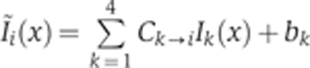of the ith control experiment was computed, where the mean intensities I_k(x) were approximated to first order by the measured mean intensities , with all secondary antibodies present. Coefficients c_k→i and b_k were obtained by minimizing the Euclidean distance between and for any channel i. The final C_k→I’s and the b_k’s are given by

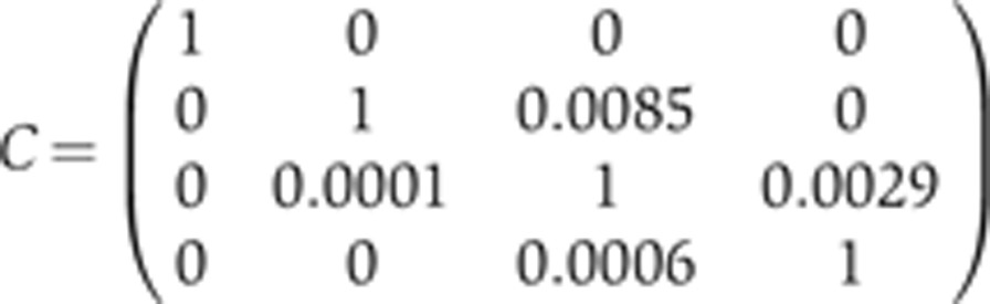and B=(73.7 0 0 0), where the the element C_k,i of the matrix represents the contribution of the kth fluorophore (Alexa-488, Alexa-568, Alexa-594, and Alexa-647, respectively) to the ith optical channel (520/40, 575/20, 620/40, and 670/40, respectively). The corresponding estimated mean control profiles are plotted in black dashed lines on the bottom panel of Figure 1D.

Systematic error analysis: 6. Focal plane determination

For each individual embryo, the focal plane has to be hand adjusted before image acquisition. Using the bright field channel, we adjust the focal plane to be at the midsagittal plane of the embryo but estimate our uncertainty to be 6 μm, or one nuclear diameter. The resulting error is estimated by computing the variances of nuclear intensities across seven images taken at consecutive heights spaced by 1 μm in a single embryo.

Determination of boundary positions and peaks in gene expression

Semi-automatic identification of expression peaks

Each raw intensity profile was binned (1000 points) and linearly filtered by computing, for each bin, the average intensity taken over the 30 nearest neighbor bins (corresponding to 3% EL, or approximately two internuclear distances). The effect of this operation is to limit intensity variations due to the presence of the nuclei and thus to compute an average nuclear/cytoplasmic intensity. A region of N bins around the presumed boundary was manually identified (e.g., 60–100% E.L, or N=400 bins for the posterior stripe of Hb). To avoid identifying local extrema solely due to higher nuclear concentrations, we randomly picked up N/3 uniformly distributed bins in that region, and computed the peak intensities and positions over the 10% intensity of highest (respectively, lowest) bins. We similarly defined for each embryo and each profile the maximum intensity I_max as well as the background intensity I_min.

Boundary identification

A region of N bins was manually identified at the presumed location of the half-maximum intensity point of the boundary (e.g., 30–70% EL, or N=400 bins, for the main border of hb). The code required the finding of two neighboring data points in that region with higher and lower intensities than (I_max+I_min)/2 (given the sharp slope of the border, false positives were extremely rare and manually corrected). The intensity and position of the half-maximum amplitude bin was then identified as the mean intensity and position of the two neighboring points. The slope was determined by fitting the points in the 3% EL neighboring region with a straight line (which corresponds to approximately two internuclear distances).

Influence of age and orientation on marker reproducibility

To address the contribution of our sorting method to the value and constancy of σ_x/L, we compared our results to the reproducibility that is achieved across 163 quadruply stained embryos, without proper age and orientation classification (gray data points in Supplementary Figure 6A). In this case, we find that the s.d. across embryos is on average more than twice as large as in our original measurement, which can be explained by the fact that σ(x/L) includes the dependence of time in the profiles along the entire n.c. 14, as well as the dependence on embryo orientation w.r.t. the dorsal side. The resulting reproducibility of the markers as a function of x/L tends to be higher at the anterior and posterior ends of the embryo, where the orientation greatly influences the patterns of gene expression and where the time shift of the markers is most important.

Reproducibility quantification of Bcd and the pair-rule genes

The reproducibility of Bcd was quantified by averaging the effective r.m.s. error σ(x) in positional readout over the 20–60% EL region (15 embryos live-imaged 15 min after entry into mitosis 13, Gregor et al, 2007a). The reproducibility of the pair-rule genes was quantified by measuring the s.d. of the position of the peaks of the seven stripes of Even-Skipped and Runt across 12 embryos selected in a 40–50-min time window after the beginning of n.c. 14 (Dubuis et al, 2011; Dubuis, 2012).

Computation of σ_x

For a single gene g, we compute the positional error for 100 equally spaced positions along the AP axis, using 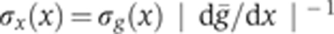(Dubuis et al, 2011; Dubuis, 2012). At each point, the error bars on the positional error are estimated by bootstrapping over 10 samples of size , where is the number of profiles collected for gene g. Supplementary Figure 7 illustrates this procedure geometrically for the case of Hb (Supplementary Figure 7A) and Kr (Supplementary Figure 7C). The positional error at a given x can be visualized as the AP distance between the intersection points of and a rectangle of width σ_g(x). The positional error is smaller in regions where the expression profile slopes are large, and hence where gene expression variations are reliably translated into variations in position (Supplementary Figure 7B and D).

In a straightforward generalization of the single gene case, the positional error for the multiple gene case is given by:

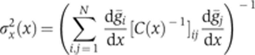where C_ij is the covariance matrix of the profiles that is directly estimated from the quadruple staining at each position x. An illustration for two genes (Hb and Kr) is shown in Supplementary Figure 7E and F. The positional error at a given x can be visualized as the AP distance between the positions of the intersection points of and a cylinder whose base is the ellipsoid in the {hb,kr} plane such that 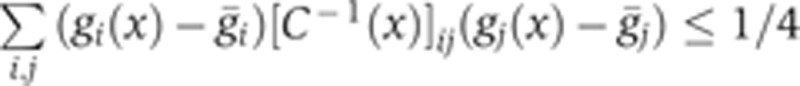. Note that the optimal positional decoding performed with several genes (e.g., N=2) at a given x does not correspond to the positional error carried by the gene with the least individual positional error at that position, i.e., the combined error can be smaller than the individual errors owing to the noise averaging by the N readouts and the correlation structure of the profiles.

Data availability

The following data have been deposited in the Dryad repository: http://dx.doi.org/10.5061/dryad.35h8v. (1) For each measured embryo, the individual raw and processed dorsal expression profiles, as well as the measured depth, of the membrane FC and the resulting inferred developmental time. (2) A table that provides the calibration curve for the time-dependent furrow depth. (3) The full set of images (with labels that allow to link the images to the profiles supplied).

Supplementary Material

Supplementary Information

Supplementary Figures S1–7

Supplementary Video 1

Membrane furrow canal invagination

Supplementary Video 2

Dynamics of the four main gap gene expression profiles

References

- Akam M (1987) The molecular basis for metameric pattern in the Drosophila embryo. Development 101: 1–22 [PubMed] [Google Scholar]
- Alexandre C, Lecourtois M, Vincent J (1999) Wingless and Hedgehog pattern Drosophila denticle belts by regulating the production of short-range signals. Development 126: 5689–5698 [DOI] [PubMed] [Google Scholar]
- Arias AM, Hayward P (2006) Filtering transcriptional noise during development: concepts and mechanisms. Nat Rev Genet 7: 34–44 [DOI] [PubMed] [Google Scholar]
- Ay A, Fakhouri WD, Chiu C, Arnosti DN (2008) Image processing and analysis for quantifying gene expression from early Drosophila embryos. Tissue Eng Part A 14: 1517–1526 [DOI] [PMC free article] [PubMed] [Google Scholar]
- Capovilla M, Eldon ED, Pirrotta V (1992) The giant gene of Drosophila encodes a b-ZIP DNA-binding protein that regulates the expression of other segmentation gap genes. Development 114: 99–112 [DOI] [PubMed] [Google Scholar]
- Choi Y, Kim HP, Hong SM, Ryu JY, Han SJ, Song R (2009) In situ visualization of gene expression using polymer-coated quantum-dot-DNA conjugates. Small 5: 2085–2091 [DOI] [PubMed] [Google Scholar]
- Clyde DE, Corado MSG, Wu X, Paré A, Papatsenko D, Small S (2003) A self-organizing system of repressor gradients establishes segmental complexity in Drosophila. Nature 426: 849–853 [DOI] [PubMed] [Google Scholar]
- Crauk O, Dostatni N (2005) Bicoid determines sharp and precise target gene expression in the Drosophila embryo. Curr Biol 15: 1888–1898 [DOI] [PubMed] [Google Scholar]
- Crombach A, Wotton KR, Cicin-Sain D, Ashyraliyev M, Jaeger J (2012) Efficient reverse-engineering of a developmental gene regulatory network. Plos Comput Biol 8: e1002589. [DOI] [PMC free article] [PubMed] [Google Scholar]
- de Lachapelle AM, Bergmann S (2010) Precision and scaling in morphogen gradient read-out. Mol Syst Biol 6: 351. [DOI] [PMC free article] [PubMed] [Google Scholar]
- Dickinson ME, Bearman G, Tille S, Lansford R, Fraser SE (2001) Multi-spectral imaging and linear unmixing add a whole new dimension to laser scanning fluorescence microscopy. BioTechniques 31: 1272–1278 [DOI] [PubMed] [Google Scholar]
- Driever W, Nüsslein-Volhard C (1988) The bicoid protein determines position in the Drosophila embryo in a concentration-dependent manner. Cell 54: 95–104 [DOI] [PubMed] [Google Scholar]
- Driever W, Thoma G, Nüsslein-Volhard C (1989) Determination of spatial domains of zygotic gene expression in the Drosophila embryo by the affinity of binding sites for the bicoid morphogen. Nature 340: 363–367 [DOI] [PubMed] [Google Scholar]
- Drocco JA, Grimm O, Tank DW, Wieschaus E (2011) Measurement and perturbation of morphogen lifetime: effects on gradient shape. Biophys J 101: 1807–1815 [DOI] [PMC free article] [PubMed] [Google Scholar]
- Dubuis JO (2012) Quantifying positional information during early embryonic development. Ph.D. dissertation, Princeton, Princeton University
- Dubuis JO, Tkacik G, Wieschaus EF, Gregor T, Bialek W (2011) Positional information, in bits. arXiv:1201.0198v1 [q-bio.MN] [DOI] [PMC free article] [PubMed] [Google Scholar]
- Edgar BA, Odell GM, Schubiger G (1989) A genetic switch, based on negative regulation, sharpens stripes in Drosophila embryos. Dev Genet 10: 124–142 [DOI] [PubMed] [Google Scholar]
- Ephrussi A, St Johnston D (2004) Seeing is believing: the bicoid morphogen gradient matures. Cell 116: 143–152 [DOI] [PubMed] [Google Scholar]
- Erdmann T, Howard M, ten Wolde PR (2009) Role of spatial averaging in the precision of gene expression patterns. Phys Rev Lett 103: 258101. [DOI] [PubMed] [Google Scholar]
- Fakhouri WD, Ay A, Sayal R, Dresch J, Dayringer E, Arnosti DN (2010) Deciphering a transcriptional regulatory code: modeling short-range repression in the Drosophila embryo. Mol Syst Biol 6: 341. [DOI] [PMC free article] [PubMed] [Google Scholar]
- Fowlkes CC, Hendriks CLL, Keränen SVE, Weber GH, Rübel O, Huang MY, Chatoor S, DePace AH, Simirenko L, Henriquez C, Beaton A, Weiszmann R, Celniker S, Hamann B, Knowles DW, Biggin MD, Eisen MB, Malik J (2008) A quantitative spatiotemporal atlas of gene expression in the Drosophila blastoderm. Cell 133: 364–374 [DOI] [PubMed] [Google Scholar]
- Gergen JP, Wieschaus EF (1986) Localized requirements for gene activity in segmentation of Drosophila embryos—analysis of armadillo, fused, giant and unpaired mutations in mosaic embryos. Wilhelm Rouxs Arch Dev Biol 195: 49–62 [DOI] [PubMed] [Google Scholar]
- Gregor T, Tank DW, Wieschaus EF, Bialek W (2007a) Probing the limits to positional information. Cell 130: 153–164 [DOI] [PMC free article] [PubMed] [Google Scholar]
- Gregor T, Wieschaus EF, McGregor AP, Bialek W, Tank DW (2007b) Stability and nuclear dynamics of the bicoid morphogen gradient. Cell 130: 141–152 [DOI] [PMC free article] [PubMed] [Google Scholar]
- Gursky VV, Panok L, Myasnikova EM, Manu, Samsonova MG, Reinitz J, Samsonov AM (2011) Mechanisms of gap gene expression canalization in the Drosophila blastoderm. BMC Syst Biol 5: 118. [DOI] [PMC free article] [PubMed] [Google Scholar]
- Hatini V, Bokor P, Goto-Mandeville R, DiNardo S (2000) Tissue- and stage-specific modulation of Wingless signaling by the segment polarity gene lines. Genes Dev 14: 1364–1376 [PMC free article] [PubMed] [Google Scholar]
- He F, Wen Y, Deng J, Lin X, Lu LJ, Jiao R, Ma J (2008) Probing intrinsic properties of a robust morphogen gradient in Drosophila. Dev Cell 15: 558–567 [DOI] [PMC free article] [PubMed] [Google Scholar]
- Held LI (1991) Bristle patterning in Drosophila. BioEssays 13: 633–640 [DOI] [PubMed] [Google Scholar]
- Houchmandzadeh B, Wieschaus E, Leibler S (2002) Establishment of developmental precision and proportions in the early Drosophila embryo. Nature 415: 798–802 [DOI] [PubMed] [Google Scholar]
- Hülskamp M, Pfeifle C, Tautz D (1990) A morphogenetic gradient of hunchback protein organizes the expression of the gap genes Krüppel and knirps in the early Drosophila embryo. Nature 346: 577–580 [DOI] [PubMed] [Google Scholar]
- Ingham PW (1988) The molecular genetics of embryonic pattern formation in Drosophila. Nature 335: 25–34 [DOI] [PubMed] [Google Scholar]
- Jaeger J (2011) The gap gene network. Cell Mol Life Sci 68: 243–274 [DOI] [PMC free article] [PubMed] [Google Scholar]
- Jaeger J, Blagov M, Kosman D, Kozlov KN, Manu, Myasnikova E, Surkova S, Vanario-Alonso CE, Samsonova M, Sharp DH, Reinitz J (2004a) Dynamical analysis of regulatory interactions in the gap gene system of Drosophila melanogaster. Genetics 167: 1721–1737 [DOI] [PMC free article] [PubMed] [Google Scholar]
- Jaeger J, Surkova S, Blagov M, Janssens H, Kosman D, Kozlov KN, Manu, Myasnikova E, Vanario-Alonso CE, Samsonova M, Sharp DH, Reinitz J (2004b) Dynamic control of positional information in the early Drosophila embryo. Nature 430: 368–371 [DOI] [PubMed] [Google Scholar]
- Jones WM, Bejsovec A (2005) RacGap50C negatively regulates wingless pathway activity during Drosophila embryonic development. Genetics 169: 2075–2086 [DOI] [PMC free article] [PubMed] [Google Scholar]
- Keränen SVE, Fowlkes CC, Hendriks CLL, Sudar D, Knowles DW, Malik J, Biggin MD (2006) Three dimensional morphology and gene expression in the Drosophila blastoderm at cellular resolution II: dynamics. Genome Biol 7: R124. [DOI] [PMC free article] [PubMed] [Google Scholar]
- Kerszberg M, Wolpert L (2007) Specifying positional information in the embryo: looking beyond morphogens. Cell 130: 205–209 [DOI] [PubMed] [Google Scholar]
- Kosman D, Mizutani CM, Lemons D, Cox WG, McGinnis W, Bier E (2004) Multiplex detection of RNA expression in Drosophila embryos. Science 305: 846. [DOI] [PubMed] [Google Scholar]
- Kosman D, Small S (1997) Concentration-dependent patterning by an ectopic expression domain of the Drosophila gap gene knirps. Development 124: 1343–1354 [DOI] [PubMed] [Google Scholar]
- Kosman D, Small S, Reinitz J (1998) Rapid preparation of a panel of polyclonal antibodies to Drosophila segmentation proteins. Dev Genes Evol 208: 290–294 [DOI] [PubMed] [Google Scholar]
- Kraut R, Levine M (1991) Spatial regulation of the gap gene giant during Drosophila development. Development 111: 601–609 [DOI] [PubMed] [Google Scholar]
- Kudoh T, Tsang M, Hukriede NA, Chen X, Dedekian M, Clarke CJ, Kiang A, Schultz S, Epstein JA, Toyama R, Dawid IB (2001) A gene expression screen in zebrafish embryogenesis. Genome Res 11: 1979–1987 [DOI] [PubMed] [Google Scholar]
- Lacalli TC, Wilkinson DA, Harrison LG (1988) Theoretical aspects of stripe formation in relation to Drosophila segmentation. Development 104: 105–113 [DOI] [PubMed] [Google Scholar]
- Lander AD (2007) Morpheus unbound: reimagining the morphogen gradient. Cell 128: 245–256 [DOI] [PubMed] [Google Scholar]
- Lander AD (2011) Pattern, growth, and control. Cell 144: 955–969 [DOI] [PMC free article] [PubMed] [Google Scholar]
- Lawrence PA (1992) The Making of a Fly: the Genetics of Animal Design. Oxford, Blackwell Scientific. [Google Scholar]
- Lecuit T, Samanta R, Wieschaus E (2002) Slam encodes a developmental regulator of polarized membrane growth during cleavage of the Drosophila embryo. Dev Cell 2: 425–436 [DOI] [PubMed] [Google Scholar]
- Lein ES, Hawrylycz MJ, Ao N, Ayres M, Bensinger A, Bernard A, Boe AF, Boguski MS, Brockway KS, Byrnes EJ, Chen L, Chen L, Chen TM, Chin MC, Chong J, Crook BE, Czaplinska A, Dang CN, Datta S, Dee NR et al. (2007) Genome-wide atlas of gene expression in the adult mouse brain. Nature 445: 168–176 [DOI] [PubMed] [Google Scholar]
- Little SC, Tkacik G, Kneeland TB, Wieschaus EF, Gregor T (2011) The formation of the bicoid morphogen gradient requires protein movement from anteriorly localized mRNA. PLoS Biol 9: e1000596. [DOI] [PMC free article] [PubMed] [Google Scholar]
- Ludwig MZ, Manu, Kittler R, White KP, Kreitman M (2011) Consequences of eukaryotic enhancer architecture for gene expression dynamics, development, and fitness. Plos Genet 7: e1002364. [DOI] [PMC free article] [PubMed] [Google Scholar]
- Manu, Surkova S, Spirov AV, Gursky VV, Janssens H, Kim AR, Radulescu O, Vanario-Alonso CE, Sharp DH, Samsonova M, Reinitz J (2009a) Canalization of gene expression and domain shifts in the Drosophila blastoderm by dynamical attractors. Plos Comput Biol 5: e1000303. [DOI] [PMC free article] [PubMed] [Google Scholar]
- Manu, Surkova S, Spirov AV, Gursky VV, Janssens H, Kim AR, Radulescu O, Vanario-Alonso CE, Sharp DH, Samsonova M, Reinitz J (2009b) Canalization of gene expression in the Drosophila blastoderm by gap gene cross regulation. PLoS Biol 7: e1000049. [DOI] [PMC free article] [PubMed] [Google Scholar]
- Mjolsness E, Sharp D, Reinitz J (1991) A connectionist model of development. J Theor Biol 152: 429–453 [DOI] [PubMed] [Google Scholar]
- Myasnikova E, Samsonova A, Kozlov K, Samsonova M, Reinitz J (2001) Registration of the expression patterns of Drosophila segmentation genes by two independent methods. Bioinformatics 17: 3–12 [DOI] [PubMed] [Google Scholar]
- Myasnikova E, Surkova S, Panok L, Samsonova M, Reinitz J (2009) Estimation of errors introduced by confocal imaging into the data on segmentation gene expression in Drosophila. Bioinformatics 25: 346–352 [DOI] [PMC free article] [PubMed] [Google Scholar]
- Namba R, Pazdera TM, Cerrone RL, Minden JS (1997) Drosophila embryonic pattern repair: how embryos respond to bicoid dosage alteration. Development 124: 1393–1403 [DOI] [PubMed] [Google Scholar]
- Neher RA, Mitkovski M, Kirchhoff F, Neher E, Theis FJ, Zeug A (2009) Blind source separation techniques for the decomposition of multiply labeled fluorescence images. Biophys J 96: 3791–3800 [DOI] [PMC free article] [PubMed] [Google Scholar]
- Nüsslein-Volhard C, Wieschaus E (1980) Mutations affecting segment number and polarity in Drosophila. Nature 287: 795–801 [DOI] [PubMed] [Google Scholar]
- Ochoa-Espinosa A, Yu D, Tsirigos A, Struffi P, Small S (2009) Anterior-posterior positional information in the absence of a strong bicoid gradient. Proc Natl Acad Sci USA 106: 3823–3828 [DOI] [PMC free article] [PubMed] [Google Scholar]
- Papatsenko D (2009) Stripe formation in the early fly embryo: principles, models, and networks. BioEssays 31: 1172–1180 [DOI] [PubMed] [Google Scholar]
- Papatsenko D, Levine M (2011) The Drosophila gap gene network is composed of two parallel toggle switches. PloS One 6: e21145. [DOI] [PMC free article] [PubMed] [Google Scholar]
- Pisarev A, Poustelnikova E, Samsonova M, Reinitz J (2009) FlyEx, the quantitative atlas on segmentation gene expression at cellular resolution. Nucleic Acids Res 37: D560–D566 [DOI] [PMC free article] [PubMed] [Google Scholar]
- Reinitz J, Kosman D, Vanario-Alonso C, Sharp D et al. (1998) Stripe forming architecture of the gap gene system. Dev Genet 23: 11–27 [DOI] [PubMed] [Google Scholar]
- Reinitz J, Sharp D (1995) Mechanism of eve stripe formation. Mech Dev 49: 133–158 [DOI] [PubMed] [Google Scholar]
- Richelle J, Ghysen A (1979) Determination of sensory bristles and pattern formation in Drosophila. I. A model. Dev Biol 70: 418–437 [DOI] [PubMed] [Google Scholar]
- Rivera-Pomar R, Lu X, Perrimon N, Taubert H, Jäckle H (1995) Activation of posterior gap gene expression in the Drosophila blastoderm. Nature 376: 253–256 [DOI] [PubMed] [Google Scholar]
- Sánchez L, Thieffry D (2001) A logical analysis of the Drosophila gap-gene system. J Theor Biol 211: 115–141 [DOI] [PubMed] [Google Scholar]
- Schrödinger E (1944) What Is Life? Cambridge, UK: Cambridge University Press, [Google Scholar]
- Struhl G, Johnston P, Lawrence PA (1992) Control of Drosophila body pattern by the hunchback morphogen gradient. Cell 69: 237–249 [DOI] [PubMed] [Google Scholar]
- Surkova S, Kosman D, Kozlov K, Manu, Myasnikova E, Samsonova AA, Spirov A, Vanario-Alonso CE, Samsonova M, Reinitz J (2008) Characterization of the Drosophila segment determination morphome. Dev Biol 313: 844–862 [DOI] [PMC free article] [PubMed] [Google Scholar]
- Tassy O, Daian F, Hudson C, Bertrand V, Lemaire P (2006) A quantitative approach to the study of cell shapes and interactions during early chordate embryogenesis. Curr Biol 16: 345–358 [DOI] [PubMed] [Google Scholar]
- Thompson DAW (1917) On Growth and Form Cambridge, UK: Cambrige University Press, [Google Scholar]
- Tkacik G, Callan CG, Bialek W (2008) Information flow and optimization in transcriptional regulation. Proc Natl Acad Sci USA 105: 12265–12270 [DOI] [PMC free article] [PubMed] [Google Scholar]
- Tkacik G, Walczak AM, Bialek W (2009) Optimizing information flow in small genetic networks. Phys Rev E 80: 031920. [DOI] [PMC free article] [PubMed] [Google Scholar]
- Tomancak P, Berman BP, Beaton A, Weiszmann R, Kwan E, Hartenstein V, Celniker SE, Rubin GM (2007) Global analysis of patterns of gene expression during Drosophila embryogenesis. Genome Biol 8: R145. [DOI] [PMC free article] [PubMed] [Google Scholar]
- Tsien RY (1998) The green fluorescent protein. Annu Rev Biochem 67: 509–544 [DOI] [PubMed] [Google Scholar]
- Ulbrich MH, Isacoff EY (2007) Subunit counting in membrane-bound proteins. Nat Methods 4: 319–321 [DOI] [PMC free article] [PubMed] [Google Scholar]
- Visel A, Thaller C, Eichele G (2004) GenePaint.org: an atlas of gene expression patterns in the mouse embryo. Nucleic Acids Res 32: D552–D556 [DOI] [PMC free article] [PubMed] [Google Scholar]
- Whittle JR (1998) How is developmental stability sustained in the face of genetic variation? Int J Dev Biol 42: 495–499 [PubMed] [Google Scholar]
- Wigglesworth VB (1940) Local and general factors in the development of ‘Pattern’ in Rhodnius Prolixus (Hemiptera). J Exp Biol 17: 180–201 [Google Scholar]
Associated Data
This section collects any data citations, data availability statements, or supplementary materials included in this article.
Supplementary Materials