A Goal-Directed Spatial Navigation Model Using Forward Trajectory Planning Based on Grid Cells

Abstract

A goal-directed navigation model is proposed based on forward linear look-ahead probe of trajectories in a network of head direction cells, grid cells, place cells, and prefrontal cortex (PFC) cells. The model allows selection of new goal-directed trajectories. In a novel environment, the virtual rat incrementally creates a map composed of place cells and PFC cells by random exploration. After exploration, the rat retrieves memory of the goal location, picks its next movement direction by forward linear look-ahead probe of trajectories in several candidate directions while stationary in one location, and finds the one activating PFC cells with the highest reward signal. Each probe direction involves activation of a static pattern of head direction cells to drive an interference model of grid cells to update their phases in a specific direction. The updating of grid cell spiking drives place cells along the probed look-ahead trajectory similar to the forward replay during waking seen in place cell recordings. Directions are probed until the look-ahead trajectory activates the reward signal and the corresponding direction is used to guide goal-finding behavior. We report simulation results in several mazes with and without barriers. Navigation with barriers requires a PFC map topology based on the temporal vicinity of visited place cells and a reward signal diffusion process. The interaction of the forward linear look-ahead trajectory probes with the reward diffusion allows discovery of never before experienced shortcuts towards a goal location.

Introduction

The entorhinal cortex and hippocampus play a role in goal-directed behavior towards recently learned spatial locations in an environment. Rats show impairments in finding the spatial location of a hidden platform in the Morris water-maze after lesions of the hippocampus (Morris et al., 1982; Steele and Morris, 1999), postsubiculum (Taube et al., 1992) or entorhinal cortex (Steffenach et al., 2005). Recordings in these regions during rat behavior show neural spiking activity relevant to goal-directed spatial behavior, including grid cells in the entorhinal cortex that fire when the rat is in a repeating array of locations in the environment falling on the vertices of tightly packed equilateral triangles (Hafting et al., 2005; Moser and Moser, 2008). Recordings also show place cells in the hippocampus that respond to mostly unique spatial locations (O’Keefe, 1976; McNaughton et al., 1983; O’Keefe and Burgess, 2005), head direction cells in the postsubiculum that respond to narrow ranges of allocentric head direction (Taube et al., 1990a; Taube and Bassett, 2003), and cells that respond to translational speed of running (Sharp, 1996; O’Keefe et al., 1998). Models have simulated the generation of grid cell spiking responses using mechanisms including interference (Burgess et al., 2007; Giocomo et al., 2007; Hasselmo et al., 2007; Hasselmo, 2008) or attractor dynamics (Fuhs and Touretzky, 2006, 2006; McNaughton et al., 2006; Guanella and Verschure, 2007; Guanella et al., 2007; Burak and Fiete, 2009). A number of previous models have addressed mechanisms of goal-directed spatial behavior using biological circuits. Some models drive goal-directed spatial behavior based on modified connectivity between place cells (Touretzky and Redish, 1996; Redish and Touretzky, 1998) or between place cells and units representing behavioral motor actions (Burgess et al., 1997; Arleo and Gerstner, 2000; Foster et al., 2000; Hasselmo and Eichenbaum, 2005; Zilli and Hasselmo, 2008; Sheynikhovich et al., 2009; Duff et al., 2011). However, previous models have not used grid cells to perform goal directed planning of trajectories. The model presented here performs goal-directed forward linear look-ahead probes of potential trajectories through the environment using a circuit of head direction cells, grid cells, and place cells similar to a previous model (Hasselmo, 2008). The circuit drives the formation of a place cell map via Hebbian modification of connections between prefrontal cortex (PFC) cells to encode the environment’s topology. A reward signal then propagates through the place cell map originating from goal locations. The look-ahead trajectory of grid cells that activates place cells associated with highest reward signal can then be selected to guide behavior. The forward probing might be the underlying phenomenon of the previously reported spiking replay seen during rat waking behavior at choice points (Johnson and Redish, 2007). Both the spatial encoding and the best next direction discovery recruit the same head-direction cell, grid cell, place cell, and PFC cell circuit. One of the main contributions of our work is how the best next direction toward the chosen goal is discovered probing the diffused reward signal via forward linear look-ahead trajectory readouts emanating from the animal’s current location, while allowing discovery of never before experienced shortcuts in the environment.

Methods

In this section we present the main ideas and constructs used to develop the goal-directed navigation model of a virtual rat. First, for the sake of completeness, we explain the roles and computational models of three different neuron types, i.e., the head direction cell, the grid cell, and the place cell. We then elaborate on how these three neuron types give rise to a place cell map based on interactions with PFC cortical columns and finally show how the head direction cell, grid cell, and place cell neural circuit as shown in Figure 1, can exploit the place cell map connectivity using forward linear look-ahead trajectory probes to guide the virtual rat towards chosen goal locations.

Notation

We show scalar parameters by italic lowercase Latin characters, e.g., d, or in normal lowercase Greek characters, e.g., θ. Vectors are shown by bold lowercase characters, e.g., d. Vectors are row-wise unless specified otherwise. Matrices are shown by uppercase bold characters, e.g., W. We show an item’s position in a collection with subscripts, e.g., θ₅ or p_k. Superscript is reserved for power operations with the exception of the transpose operation, e.g., d^T. We show collections such as sets and populations by uppercase italic characters, e.g., D. Lowercase italic bold characters represent the class of the item they refer to, e.g., place cell p or grid cell g.

Head Direction Cells

A head direction cell is a neuron type specialized to significantly increase its firing rate as the allocentric head direction of the animal gets closer to a specific polar angle value which we refer to as the tuned or the preferred direction of the cell. Extensive experimental data describe head direction cells in the deep layers of the entorhinal cortex (Sargolini et al., 2006) and in other areas including the postsubiculum (Taube et al., 1990a) and the anterior thalamus (Taube, 1995). Our goal-directed navigation model uses head direction cells generating speed modulated signals: the firing rate is proportional to both the current head direction and the speed of the virtual rat. Note that in the simulations presented in this paper, we assume that head direction matches the virtual rat’s movement direction. Previous experimental data show that the tuned directions of all head direction cells of a single subject tend to be locked to a specific main orientation (Taube et al., 1990b; Knierim et al., 1995). Hence the preferred direction of the i^th head direction cell can be represented as an angular offset θ_i from a main orientation θ₀, i.e,. (θ_i=1,...,m+θ₀) , where m is the head direction cell population size. Given the tuning kernel:

$$\mathbf{D}=\left[\begin{array}{c}\hfill \cos \left({\theta }_1+\left({\theta }_0+w_d\right)\right)\cdots \cos \left({\theta }_m+\left({\theta }_0+w_d\right)\right)\hfill \\ \hfill \sin \left({\theta }_1+\left({\theta }_0+w_d\right)\right)\cdots \sin \left({\theta }_m+\left({\theta }_0+w_d\right)\right)\hfill \end{array}\right]$$ (1)

and the virtual rat’s instantaneous velocity v(t), the head direction signals can be obtained using:

$$\mathbf{d}\left(t\right)=\mathbf{v}\left(t\right)\cdot \mathbf{D}=\left[d_1\left(t\right),\dots ,d_m\left(t\right)\right]$$ (2)

Where d_i(t) is the population’s i^th member’s head direction signal at time t with preferred direction θ_i, and w_d is the error term representing the deviation from the main orientation due to noise.

Grid Cells

A grid cell is a neuron type which increases its firing rate significantly when the animal traverses a regular array of periodic places in the environment. The collection of locations where an individual grid cell fires, i.e., the grid cell’s firing fields, forms a two dimensional periodic pattern with regular inter-field intervals and similar field areas. Extensive experimental data show the existence of grid cells with different inter-field spacing and field areas along the dorsal to ventral axis of the medial entorhinal cortex (Hafting et al., 2005; Sargolini et al., 2006). In this work we use the persistent spiking model (Hasselmo, 2008) to generate grid cells’ spiking activity. The persistent spiking model belongs to the class of phase interference models.

Phase Interference Models

The phase interference models generate the grid cell’s typical grid like spatial periodic spiking activity by combining several speed modulated oscillations into a single interference pattern. In an early, single cell version of the oscillation interference model by Burgess et al. (2007) and Hasselmo et al. (2007) each dendrite of a grid cell receives its input from a population of speed modulated head direction cells tuned towards the same preferred direction. The speed modulated head direction cell inputs shift the oscillation phase of each population relative to each other. Finally, the different network oscillations are combined to drive the spiking activity of individual grid cells. Recent work suggests that this mechanism could more realistically involve interactions of different network oscillations (Zilli and Hasselmo, 2010).

In the phase interference model based on the interaction of entorhinal persistent spiking cells (Hasselmo, 2008), which is implemented and used in this work’s simulations, each population of entorhinal persistent spiking cells receive synaptic inputs from their respective head direction cell populations tuned towards the same preferred direction. Multiple persistent spiking cell populations send convergent input to an individual grid cell. Consecutively, a grid cell generates spiking activity when all its dendritic inputs receive almost simultaneous spikes from their pre-synaptic persistent spiking cell populations. We reproduce here a slight variation of the persistent spiking model from Hasselmo (2008) for the sake of completeness since it will be used to develop and explain other concepts further in this paper:

$$\begin{array}{cc}\hfill & {\varphi }_{(i,j)}\left(t\right)=2\pi \left(ft+b_j{\int }_0^t{d}_i\left(\tau \right)d\tau \right)\hfill \\ \hfill & s_{(i,j)}\left(t\right)=\mathrm{H}\left(\cos \left({\varphi }_{(i,j)}\left(t\right)+{\psi }_{(i,j)}+w_{(i,j)}\right)-s_{\mathit{thr}}\right)\hfill \\ \hfill & g_j\left(t\right)=\prod _{s\in S_j}s\left(t\right)\hfill \end{array}$$ (3)

Where H() is the Heaviside step function with H(0)=0, g_j(t) is the spiking output of the j^th grid cell at time t , S_j is the set of persistent spiking cells projecting to the j^th grid cell, s_(i,j)(t) is the output of the persistent spiking cell receiving input from i^th head direction cell and projecting to the j^th grid cell, s_thr is the spiking threshold value of all persistent spiking cells, and w_(i,j) is the noise term. The persistent spiking cell has phase offset Ψ_(i,j), intrinsic baseline frequency f, and scaling factor b_j. Note that in this model all persistent spiking cell baseline frequencies are the same.

All the simulations presented in this work are based on our persistent spiking model implementation.

Place Cells

One of the main requirements of many goal-directed navigation strategies is the existence of a place cell map representation mechanism, i.e., the ability to associate real-world locations to neuronal activities in a one-to-one fashion. Spatial representations generated by grid cells are of many-to-one nature: the firing fields of a single grid cell correspond to several periodic spatial locations. Place cells are effective candidates for the spatial representation: they mostly tend to fire exclusively inside a specific spatial area (O’Keefe, 1976; McNaughton et al., 1983; O’Keefe and Burgess, 2005) which allows the formation of a place cell map by exploring an environment.

Model

There are several models trying to explain the formation of place cells from grid cell inputs (McNaughton et al., 2006; Rolls et al., 2006; Solstad et al., 2006; Gorchetchnikov and Grossberg, 2007). These include models in which grid cells can drive place cells without requiring synaptic plasticity (Almeida et al., 2009, 2010). In our model a place cell acts as an AND gate for converging inputs from several pre-synaptic grid cells. The k^th place cell, p_k, receives its synaptic inputs from a population of grid cells, G_k, with different firing field separation and sizes. A place cell generates spikes whenever all of its inputs receive almost simultaneous spikes. The computational model for a single place cell signal is as follows:

$$p_k\left(t\right)=\mathrm{H}\left(\prod _{g\in G_k}g\left(t\right)\right)$$ (4)

While Equation 4 addresses the place cell activity mechanism, it does not yet clearly explain how:

1. A place cell’s firing field can be tuned to a unique spatial location (selectivity),

2. A place cell’s firing field can be tuned to an arbitrary spatial location (arbitrariness).

The model presented in Equation 4 accomplishes these two place cell properties by putting together populations of grid cells, G_k , with special characteristics explained next.

Selectivity

Selectivity can be defined as how unambiguously a single spatial location can be encoded by a place cell. In the ideal case a place cell should only spike at a single spatial location creating zero ambiguity and maximum selectivity. In a significant number of cases, however, physiological evidence shows multiple firing fields per place cell recorded in vivo (Fenton et al., 2008). We measure the selectivity by the number of a single place cell’s firing fields per a given area making selectivity dependent on the size and shape of the enclosed environment: A place cell with multiple firing fields might be highly selective for a smaller area but its selectivity might suffer as the environment grows larger. In our place cell model the selectivity can never be optimally maximum by construction but it can be parameterized by a number of factors, such as the number of converging grid cells and their intrinsic properties, as presented below. Each population G_k contains grid cells receiving inputs from persistent spiking cells having the same intrinsic frequency f but different scaling constants b_j. When unit-amplitude oscillations with different frequencies and identical initial phases are summed together the result is an interference oscillation with amplitudes of its highest peaks equal to the number of summed oscillations and with frequency of its highest peaks smaller than any of its components. Consider the toy example with several 1D unit amplitude cosine oscillations as shown in Figure 2. In this example, each cosine oscillation with frequency f scaled by a constant b_j has periodic peaks at instantaneous phase values which are multiples of 2π. We can represent this as follows:

$$\left(2\pi b_{j}ft\right)\mathrm{mod}2\pi =0\iff \left(b_{j}ft\right)\in Z$$ (5)

Equation 5 implies that two or more cosine oscillations with different scaling factors will be in-phase when the terms (b_jft) are simultaneously integers. If we sum these oscillations, the resultant interference pattern will have highest peaks at instantaneous phase locations where all the component oscillations simultaneously satisfy Equation 5 as shown in Figure 2 (Bottom row), with peak amplitudes equal to the number of its unit amplitude components. Equivalently, the resultant oscillation’s highest peaks will occur at instantaneous phase values equal to the common multiples of its components’ (b_jft) terms. Hence, the period of the resultant’s highest peaks will be equal to the least common multiple (lcm) (Gorchetchnikov and Grossberg, 2007) of the individual components’ periods by definition, i.e.:

$$\left(2\pi b_{j}ft\right)\mathrm{mod}2\pi =0\iff t=1\mathrm{cm}\left({\left(b_{j}f\right)}^{-1}\right)\text{where}j=1,\dots ,\mid G_k\mid \wedge \left(b_{j}f\right)\in \mathrm{Q}$$ (6)

Note that since least common multiple is defined for the set of rational numbers we limit the domain of the frequencies to rational numbers. As a result of this analysis we observe the following characteristics of the resultant signal:

1. The frequency of the resultant can be made arbitrarily smaller than any of its components’ frequencies. The summation of oscillations with different scaling factors creates a resultant oscillation with relatively dampened peak amplitudes in the half-period neighborhood of its highest peaks. If we apply an appropriate threshold to the resultant signal (or to the component signals before summation), we obtain a pulse wave with a much larger period than any of its components.

2. The presented analysis is also valid when the continuous sinusoid signals are thresholded to produce pulse waves and the summation operation is replaced by the product operation. The product of pulse waves with different scaling factors generates a resultant pulse wave with frequency significantly smaller than any of its components.

3. In the discrete case, the resultant pulse wave’s single pulse duration is equal to the minimum of its components’ single pulse durations. This characteristic can be exploited in the parameterization of a place cell’s firing field size.

Even though characteristics one and two do not provide a signal with a globally unique peak or spike train location, they do guarantee an ideal selectivity up to some neighborhood range which can be parameterized by the number and the scaling constants of its component oscillations. The analysis provided for 1D cosine signals also extends to the 2D case where the component cosine signals are replaced by grid cell firing fields and the resultant signal is replaced by the place cell firing field(s).

Arbitrariness

We define the arbitrariness as the ability to tune a place cell’s firing field to an arbitrary spatial location. We accomplish this by exploiting the translational effect of the phase offset value Ψ_(j,i) of Equation 3 on the grid cell firing fields. In the persistent spiking model, each persistent spiking cell is in phase with a reference oscillation at a baseline frequency. As the animal moves in the environment, the velocity modulated head direction signals shift the phases of the respective persistent spiking cells relative to the reference oscillation. While the raw spiking activity of a persistent spiking cell population modulated by head direction cells tuned to the same direction will not show any location selectivity, their phase shift relative to the spikes of the reference oscillation will show band like patterns (Hasselmo, 2008). The grid cell receiving inputs from different persistent spiking cell populations will fire only when all its inputs fire almost simultaneously, i.e., at spatial locations where all the bands seen in Hasselmo (2008) coincide. In light of these observations, we can conclude that by methodically translating the locations of these bands (or equivalently by shifting the phase of persistent spiking cells by constant offsets), we can translate the locations of a grid cell’s firing fields. Furthermore, by finding a mapping from the phase offset amount onto the firing field translation amounts, we can parameterize the firing fields’ spatial locations. The phase offset translating the grid cell j [Δx, Δy] units in Cartesian space is:

$${\Psi }_{(i,j)}=-2\pi \left(f+b_j[\Delta x,\Delta y]\left[\begin{array}{c}\hfill \cos \left({\theta }_i\right)\hfill \\ \hfill \sin \left({\theta }_i\right)\hfill \end{array}\right]\right)$$ (7)

The minus sign in front of the Equation 7’s right-hand-side is necessary since translating an oscillation to the right is equivalent for its phase to shift at an earlier offset. In summary, application of the Equation 7 to all persistent spiking cells converging to the j^th grid cell translates the grid cell’s firing fields by the given amount in the Cartesian space hence achieving the arbitrariness.

Place Cell Map

In our navigation model the place cell map is a collection of prefrontal cortex cortical columns bijectively connected to the hippocampal place cells as shown in Figure 3. Cortical columns of the prefrontal cortex have been included in previous models of goal directed behavior where, similar to our model, spread of reward activity drives selection of the next motor activity towards the achievement of a goal state (Gorchetchnikov and Hasselmo, 2005; Hasselmo, 2005). Previous experimental work reported observation of place-cell like activity confined to specific regions of the behavioral environment in recordings from the medial prefrontal cortex (mPFC) during goal directed navigation planning in rats (Hok et al., 2005). Furthermore, experimental papers have also reported observations of anticipatory firing of rat mPFC cells prior to achievement of a goal such as release of food pellets, (Burton et al., 2009), similar to the anticipatory firing of dorsal hippocampal cells (Hok et al., 2007). Bilateral lesions of the ventral and intermediate hippocampus reduce the mPFC activity suggesting co-operation between the hippocampus and PFC during goal directed activity (Burton et al., 2009). This co-operation is also supported by recordings showing that firing of mPFC neurons is phase-locked to hippocampal theta rhythm (Hyman et al., 2005; Jones and Wilson, 2005). Experimental data also supports a potential role of rat prefrontal cortex neurons in maintenance of working memory during goal directed tasks (Baeg et al., 2003).

In our model each PFC cortical column contains three cell layers connected to each other: A recency cell layer Q, a topology cell layer U, and a reward cell layer R. The recency layer cell q_k maintains the recency signal q_k associated to the place cell p_k. The recency signals are used to update the lateral connections among the topology layer cells. The topology cell layer’s lateral connections are updated incrementally as the virtual rat experiences its environment. They represent the environment’s spatial topology in the PFC. The reward layer cell r_k maintains the reward signal r_k associated to the place cell p_k The reward signals play a crucial role in planning navigation directions towards previously visited goal locations such as food sources or safe places. The functionality of all PFC cortical column cell types and signals are explained in detail below.

The PFC cortical column’s topology layer cells are connected to each other via lateral connections represented by the adjacency matrix W_u. The place cell map encodes the spatial topology of the environment’s visited areas via lateral connections enabling the reward signal diffusion process. When the virtual rat is first introduced to a never before experienced environment the corresponding place cell map is incrementally generated by recruiting new place cells and PFC cortical columns and updating the respective PFC signals accordingly. While hippocampal place cells provide raw information about the virtual rat’s location, e.g., “I am at location D”, the PFC cortical columns augment the hippocampal information by the neighborhood context, e.g., “I am at location D which is close to locations A, B, and F”. For the rest of the paper the recruitment of a new place will also imply the recruitment of a new PFC cortical column and vice versa.

Place Cell Recruitment

When the virtual rat is introduced to a never before experienced environment, a place cell p₀ is recruited receiving its synaptic inputs from a population of grid cells, G₀, with zero phase offset vectors representing the virtual rat’s original starting position. The G₀’s grid cells’ phases act also as an anchor point in the recruitment of the successive grid cells in the same environment. As the virtual rat explores the new environment following a smoothed random walk trajectory, it incrementally recruits new place cells. What triggers the exclusive representation of a spatial location by a place cell is still an open question. In our implementations the virtual rat recruits new place cells either deterministically or in a pseudo-random fashion: In the deterministic case the virtual rat recruits a new place cell as soon as it enters a location in the environment which is not represented by any other existing place cell. This approach creates a relatively dense representation since all place fields are highly overlapping. In the pseudo-random case the virtual rat recruits a new place cell when (i) the location is not represented by any other place cell as in the deterministic case and (ii) a sample drawn at each time step from a probability distribution is smaller than a given threshold value. In the pseudo-random case the density of the place cell firing fields is parameterized by the probability distribution and the threshold value. Examples for both triggering mechanisms are given in Figure 4.

Recruitment of a new place cell also means recruitment of a new grid cell set and their respective presynaptic persistent spiking cells. The virtual rat tunes the new place cell to its current location by recruiting a new set of grid cells which are the translated versions of the very first grid cell set G₀. The translation is equivalent to setting the new grid cells’ phase and phase offset vectors to G₀ grid cells’ phase vectors and to their additive inverses, i.e.:

$$\begin{array}{cc}\hfill & G_{k+1}=\left\{g_{(k+1,1)},\dots ,g_{(k+1,j)},\dots ,g_{(k+1,n)}\right\}\hfill \\ \hfill & S_{(k+1,j)}=\left\{s_{(k+1,1,j)},\dots ,s_{(k+1,i,j)},\dots ,s_{(k+1,m,j)}\right\}\hfill \\ \hfill & {\varphi }_{(k+1,i,j)}={\varphi }_{(0,i,j)}\hfill \\ \hfill & {\Psi }_{(k+1,i,j)}=-{\varphi }_{(0,i,j)}\hfill \end{array}$$ (8)

Where n is the number of grid cells feeding synaptic input to a single place cell and m is the head direction cells.

Temporal Neighborhood Topology

We impose a topology on the place cell map by creating lateral connections among PFC’s topology layer cells as shown in Figure 3. Each newly recruited place cell p_k is associated with a new PFC column containing a recency cell q_k with recency signal q_k, a topology cell, and a reward cell r_k with reward signal r_k. The recency signal value q_k is proportional to the elapsed time from the virtual rat’s most recent visit to the place cell p_k. As long as the virtual rat is in the firing field of some place cell p_k the corresponding recency signal q_k stays at 1. Otherwise, at each time step, q_k slowly leaks towards zero following an exponential decay with parameter ε and decay rate λ which are constant for all recency cells. The value of the recency signal q_k Δt time units after the virtual rat’s last visit to place cell p_k is:

$$q_k\left(\Delta t\right)={\epsilon }^{-\lambda \Delta t}$$ (9)

Each time the virtual rat visits a place cell p_k, the topology layer’s lateral connections are reinforced by Hebbian updates using the following equation:

$${\mathbf{W}}_u={\mathbf{W}}_u\vee \mathrm{H}\left({\mathbf{q}}^{\mathrm{T}}-\delta \right)\cdot \mathrm{H}(\mathbf{q}-1)$$ (10)

Where q=[q_i]_i=1,...,k is the recency signal vector, δ is the recency signal threshold, H() is the Heaviside step function with H(0)=1, and V is the element wise OR operator. Equation 10 updates the topology layer’s lateral connections by introducing or reinforcing connections between the currently visited PFC topology cells, represented by the indicator vector H(q-1), and the recently visited PFC topology cells, represented by the indicator vector H(q^T-δ). The threshold δ determines the time window for a PFC topology cell to be considered as recently visited. The use of the recency effect for the connection updates, in a strictly algebraic sense, imposes a temporal neighborhood disc with radius δ surrounding each place cell (recall that there is a one-to-one relationship between place cells and the PFC cortical column cells). This neighborhood relationship is not necessarily metric so the graph induced by W_u is not necessarily planar. The recency signals are time based and hence they depend on the virtual rat’s speed and the arc-length of the trajectory taken while visiting consecutive place cells.

Navigating To A Goal

So far we laid down the necessary foundation for the goal-directed navigation model by showing:

1. How grid cells emerge using head direction cell inputs and place cells emerge using grid cell inputs.

2. How the presented place cell model is both selective and arbitrary.

3. How the place cell map can abstractly represent an environment’s topology using PFC cortical columns as its main components.

4. 4. How a temporal recency effect can be used to connect PFC cortical columns by Hebbian updates. In this section, we present our navigation model that can:

   1. Pick a goal location by activating the corresponding place cells and PFC reward cells.
   2. Find the best next direction to proceed towards the goal location.

Goal Representation

We define a goal as a task specific spatial location in the environment such that the virtual rat’s arrival to that location is considered success. The virtual rat may reach a goal in two ways: i) By chance, during random exploration of a new environment when the goal location is not yet represented in the place cell map, e.g., reaching a submerged platform in a Morris water-maze task during the first trial, ii) By strategy, following a predefined deterministic strategy made possible by the virtual rat’s recent interactions with the goal and the environment, e.g., reaching the same submerged platform after several trials. In our navigation model we represent goals by PFC reward cells and their respective reward signals r=[r_i]_i=1,...,k. In this context a place cell p_k connected to a PFC column with reward signal equal to 1 represents a goal location. Hence when the virtual rat decides on a goal location it sets the corresponding reward cell’s reward signal value to 1.

Forward Linear Look-Ahead Trajectory Probes

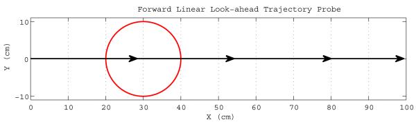
Once the reward signals are activated, the virtual rat decides on what direction to proceed to reach the goal by probing several forward linear look-ahead trajectory probes with different headings starting from its current location with range ρ^probe as shown in Figure 5. Note that each forward linear look-ahead trajectory probe fully engages the head direction cell → persistent spiking cell → grid cell → place cell circuit as if the virtual rat were physically moving along the probe trajectory, but on a faster scale possibly in a couple of theta rhythm cycles, without any behavioral locomotion. The location of the rat, during actual navigation or forward linear look-ahead trajectory probing, is represented by shifts of the phase of individual persistent spiking neurons relative to their baseline rhythm with frequency f. During the normal navigation this baseline rhythm is in the theta band, 7Hz in our simulations. During forward linear look-ahead trajectory probes each persistent spiking cell’s intrinsic baseline frequency f jumps to around Gamma band, 200Hz in our simulations, while the velocity modulated head direction input d_j is scaled up significantly by increasing its respective scaling constant b_j. The scaling constant b_j is inversely proportional to the duration of a forward linear look-ahead trajectory probe. Hence manipulation of the scaling constant b_j allows the model to arbitrarily shorten the duration of a complete cycle of linear look-ahead trajectory probe scan. For instance, at constant speed of 20 cm/s the virtual rat can travel 100 centimeters in 5 seconds on a straight line during actual navigation. During linear look-ahead trajectory scan phase the same amount of distance (100cm) can be covered by a single probe in 100 milliseconds, Figures 6 and 7, if the scaling constant b_j increases 50 times and in 10 milliseconds if b_j increases 500 times. Furthermore, the number of linear look-ahead trajectory probes might also be synchronized by the overall theta rhythm. For instance, if theta frequency is 7Hz it would take less than 2 seconds to complete a complete scan of 20 probes at a rate of 2 probes per theta cycle. The use of theta rhythm during the model’s forward linear look-ahead trajectory probing is supported by the presence of theta rhythm during forward replay in neurophysiological recordings (Johnson and Redish, 2007) and in stationary animals attending to salient stimuli (Sainsbury et al., 1987). However, in our simulations we do not use theta oscillation to synchronize the number of probes. Exceptions to the virtual rat’s immobility during the probe may involve turning to different directions as in vicarious trial-and-error (Johnson and Redish, 2007). The forward linear look-ahead trajectory probes generate spiking activity that can be observed as the virtual rat “thinking of following” a linear trajectory. In these simulations, during each forward linear look-ahead trajectory probe the speed modulated head direction activity represents a constant radial direction and speed (though they could conceivably be shifted). The constant speed modulated head direction activity causes a linear shift in the phase of persistent spiking cells that cause periodic activity of different grid cells. This causes sequential activation of place cells that are on the linear trajectory coded by the grid cell phase as shown in Figure 7.

If the place cell(s) connected to reward cells with active reward signals (representing the goal location) start to spike during a forward probe then the virtual rat proceeds in the direction of the forward probe directly leading to the goal location. Note that activation of goal place cell(s) by a forward probe conveys only directional information but not range. As soon as any goal place cell starts to spike during the virtual rat’s translational motion the goal is considered to be achieved.

The full engagement of the head direction cell → persistent spiking cell → grid cell → place cell circuit during forward linear look-ahead trajectory probes requires a mechanism to store the actual state of the network, i.e., oscillation phases, etc., before the probe and to restore it after the probe. We assume this mechanism but do not explicitly model it.

One of the advantages of this probing approach is that it does not require the explicit long-term storage of any directional information in the place cell map concerning the navigation direction from one place cell firing field to another as proposed in some of the previous approaches (Redish and Touretzky, 1998; Foster et al., 2000). Our model requires a very short-term storage of the navigation network state during the forward probing. Furthermore, our model does not require storage of fixed route vectors between place cells and goal locations. Instead, the virtual rat can pick any place cell as a goal location and decide on its next movement direction based on the topology of the place cell map. The discovered goal direction is a close approximation to the real integrated direction from the virtual rat’s current location towards the goal, thereby allowing the virtual rat to find shortcuts in the environment.

Reward Signal Diffusion

Nevertheless, there is an important limitation with this version of the goal-directed navigation approach: The goal place cell is not necessarily guaranteed to be in the range ρ^probe of the forward probes. Thus, a full scan might be unable to activate the goal place cell hence forcing the virtual rat into random exploration. One way of dealing with this issue is to expand the probe range, increasing a probe’s chances to reach the goal location. However, this approach has the following caveats:

1. We could guarantee activation of the goal place cell by at least one probe if we would be able to set the probe range to half the diameter of the graph induced by place cell map’s topology layer’s lateral connections. But since the place cell map topology is not necessarily planar any computed graph diameter would be meaningless for this purpose.

2. A longer probe range would require a longer engagement of the head direction cell → persistent spiking cell → grid cell → place cell circuit which would be highly prone to the degrading effects of accumulated signal noise in the absence of corrective inputs from other sensor modalities, e.g., visual, tactile, olfactory, etc., (Zilli et al., 2009).

3. The direction towards the goal might be obstructed.

We address these issues by allowing the virtual rat to reach the final goal in several steps following a reward signal gradient obtained by a diffusion process.

The main idea of reward diffusion is to create a gradient in the place cell map allowing the virtual rat to iteratively hill-climb through intermediate goals and finally reach the hill’s summit, i.e., the final goal. Starting with the reward signal vector where only the reward cells associated with the goal place cells have value 1 and all others 0, the diffusion process update equations are as follows:

$$\begin{array}{cc}\hfill & \mathbf{a}\left(0\right)=\mathbf{r}\hfill \\ \hfill & \alpha \left(t\right)={(t+1)}^{-1}\hfill \\ \hfill & \mathbf{a}\left(t\right)=\mathrm{H}\left(\mathbf{a}(t-1)\cdot {\mathbf{W}}_u\right)\hfill \\ \hfill & r_k=\max \left(a_k\left(t\right)\cdot \alpha \left(t\right),r_k(t-1)\right)\hfill \end{array}$$ (11)

Where a(t) is the indicator vector for PFC reward cells visited at t^th diffusion iteration, H() is the Heaviside step function with H(0)=0, and α(t) is the diffusion decay value which can be any monotonically decreasing function. The diffusion is implemented in a breadth-first fashion visiting all connected reward cells of the place cell map. The adjacency matrix W_u is not necessarily symmetric by construction. If preferred, this can be accomplished by an OR operation between H(W_u) and its transpose. The maximum operator in Equation 11 guarantees that the reward signal is updated only during the first diffusion visit of each reward cell, since the place cell map is not necessarily acyclic.

The diffusion process happens once just after the selection of a new goal location. After diffusion, the virtual rat performs several forward linear look-ahead trajectory probes and moves toward the probe direction that activates place cell associated with PFC reward cell having maximum reward signal among all place cells activated by all probes. A probe is parameterized by its egocentric direction θ_i and range ρ^probe. More specifically, the direction θ satisfying the following equation, where PROBE_θ is the set of indices of the place cells (equivalently of the PFC reward cells) activated by the probe emanating towards egocentric heading θ, is selected as the next movement direction towards the goal:

$$\underset{\theta }{\arg \max }=\left\{\max \left(\left\{r_{{\mathit{PROBE}}_{\theta }}\right\}\right)\right\}$$ (12)

While the number of unique probe headings during each full scan is an important parameter of the model, directions activating maximum reward signal are agnostic to the actual order in which the probes are executed. In our simulations, a complete forward linear look-ahead trajectory scan involves 100 linear look-ahead trajectory probes with egocentric directions (θ) uniformly distributed from -140 degrees to 140 degrees where 0 degrees is the virtual rat’s egocentric heading angle. More details are in the section on Simulation Environment.

If the goal place cell is not in the range of the current forward linear look-ahead trajectory probe, the virtual rat proceeds in the direction of the discovered probe for a fixed amount of distance (4 cm) and then starts another scan. Since the reward signal gradient has its peak at the final goal location by construction, the virtual rat is guaranteed to reach the goal after a finite number of steps. When the virtual rat should initiate a new probe is an open question. One potential answer is when the virtual rat encounters a novel stimulus, e.g., a novel path in the previously experienced part of the environment, another answer is when the virtual rat encounters decision points, e.g., turning points or junctions in a maze.

The reward signal diffusion approach avoids the previously noted caveats as follows:

1. The probe range can be relatively small keeping the degrading effects of signal noise accumulation at manageable levels.

2. The reward signal gradient naturally allows the virtual rat to pick the best next direction circumventing obstructions in the environment.

Shortcut Discovery

It is a natural capability of the goal-directed navigation strategy presented so far to find a shortcut to the goal location in an open field, i.e., in the absence of any obstacles in the environment. The forward linear look-ahead trajectory probe direction activating the goal place cell(s) provide the most direct way to the goal location from the virtual rat’s current location by construction. If the range of the probe is not long enough to activate the goal place cells from the virtual rat’s current location, then the virtual rat follows a piece-wise linear trajectory towards the goal visiting transient waypoints using the reward signal gradient. Even though the piece-wise trajectory is not guaranteed to be the shortest path, it is guaranteed to be not longer than any other path taken previously to the goal location from the same starting location.

The presented goal-directed navigation strategy is also capable of exploiting new shortcuts in an environment with obstacles: First the virtual rat creates a representation of the environment in its place cell map by random exploration. We assume that the virtual rat is able to detect and avoid obstacles by using sensory inputs such as its whiskers and/or its eyes. Once the virtual rat has sufficient information about the goal location it engages the forward linear look-ahead trajectory probe mechanism to reach the goal. The virtual rat probes only directions which are not obstructed in its immediate vicinity (2 cm) by an obstacle. If we remove some obstacles or parts of obstacles from the environment then the virtual rat would also be able to generate forward probes in the direction of the missing obstacles. If any of these forward probes, which were previously blocked by the removed obstacles, activates a place cell with maximum reward signal then the virtual rat will move through the newly available shortcut to reach the goal location. One important caveat in this approach is that if the range of the forward probes is less than the length of the new shortcut then the virtual rat will not be able to exploit the shortcut since no probe will be able to completely cross through the new opening. Recall that the space previously occupied by the obstacle is not yet represented by any place cell, but the forward linear look-ahead trajectory probe mediated by grid cell phase can move through regions of space not encoded by place cells until the forward probe reaches a location previously coded by a place cell.

Simulation Environment

All simulations are coded and performed using MATLAB version R2009b. For all simulations the simulations’ single iteration epoch is set to 0.02 seconds. Each place cell in the place cell map receives inputs from three unique grid cells generating firing fields with diameters around 20 cm, 40 cm, and 60 cm. During actual navigation the three grid cells receive bijective inputs from three unique persistent spiking cells having frequency (f) 7Hz, spiking threshold value (s_thr) 0.9, and scaling factors (b_j) 0.01, 0.004, and 0.002. During forward linear look-ahead trajectory probes the three persistent spiking cells’ frequencies jump to 200Hz and their scaling factors increase 100 times to 1, 0.04, and 0.02. Finally, the three persistent spiking cells receive bijective inputs from three head direction cells with preferred directions 0, 120, and 240 degrees. The recency threshold Δ is chosen such that connections between all place cells visited in the last 3 seconds and the current place cell get reinforced according to Equation 10. During each complete scan 100 forward linear look-ahead trajectory probes sequentially occur at 2.82 degrees intervals starting from -140 degrees and ending at 140 degrees where 0 degrees is the virtual rat’s egocentric heading angle. All forward linear look-ahead trajectory probe lengths are set to 200 cm.

Virtual Rat Model

We use a virtual rat for all our synthetic experiments. The virtual rat uses first order motion dynamics, i.e., constant speed and no acceleration. It also has the capability of detecting and avoiding obstacles in the environment by a limited line-of-sight mechanism. The line-of-sight mechanism can only classify the virtual rat’s egocentric directions as obstructed if an obstacle is closer than 2 cm to the virtual rat or as free if no obstacle is present in the range of 2 cm. The virtual rat has two predefined behaviors: Exploration and target seeking. The exploration behavior enables the virtual rat to experience its current environment by iteratively picking random transient waypoints in its limited line-of-sight area. The target seeking behavior directs the virtual rat to a given location in its current environment. We would like to emphasize that even though the virtual rat uses a line-of-sight based obstacle avoidance mechanism, the only inputs for the construction and utilization of the place cell map for goal navigation purposes are the virtual rat’s velocity vectors. The speed of the virtual rat throughout the simulation experiments is constant at 20 cm/s except during the forward linear look-ahead trajectory probes during which the virtual rat is stationary. Furthermore, the virtual rat performs a full scan of forward linear look-ahead trajectory probes after each 4 cm of travel during test trials.

Results

In this section we provide the results obtained by conducting several synthetic experiments using the proposed goal navigation framework in a simulated Morris water-maze (Morris et al., 1982), a Tolman maze (Tolman et al., 1992), and a hairpin maze (Alvernhe et al., 2008). More specifically, we report four sets of simulations. The first set uses simulated Morris water-maze (Morris et al., 1982) where all conditions are ideal, i.e., no noise, no obstacles. In the second set of experiments we inject noise in the head direction signals or the grid cell signals independently and compare Morris water-maze escape latencies versus the amount of noise. In the third and fourth sets of experiments, we show our system’s ability to exploit the never before experienced shortcut paths in a simulated Tolman maze (Tolman et al., 1992) and a hairpin maze (Alvernhe et al., 2008). In all trials we end the simulation and classify it as success when: i) The virtual rat touches the goal platform or ii) the virtual rat enters the firing field of a goal place cell. The virtual rat starts each set of experiments with an empty place cell map and continues to update its place cell map during both the training and test trials. The first trial of each set of experiments is a training trial where the virtual rat is expected to discover the goal platform for the first time by random exploration. We do not impose a time limit for the training trials. During each test trial we end the simulation if the virtual rat is not able to find the goal platform in less than 30 seconds.

Morris Water-maze Simulations

We conduct the virtual Morris water-maze simulations with the goal platform placed in the upper-right quadrant. The water-maze is a circular pool with diameter equal to 120 cm and the escape platform is a square area with each side equal to 18 cm.

In the first set of experiments all signals in the head direction cell, grid cell, and place cell circuit are ideal with no noise as shown in Figure 8. During the training trial of this simulation, the virtual rat performs a random exploration of the Morris water-maze until it finds the hidden platform. After the training trial, as shown in Figure 8 left, we test the performance of the model for two conditions: i) Starting from the same location as the training trial, as shown in Figure 8 center, ii) starting from several locations other than the one used in the training trial, as shown in Figure 8 right. After the random exploration of the training trial, the virtual rat is able to find a direct route towards the platform with a single scan, as expected, using the forward linear look-ahead trajectory probe approach for both test conditions, because the probe range is long enough to activate the goal place cell recruited during the training trial.

Noise Effect

The second set of experiments show the behavioral effect of head direction cell or grid cell signal noise on the performance of the navigation model. We chose to inject zero mean independent and identically distributed Gaussian noise with exponentially increasing standard deviations to the head direction signals and the grid cell signals in different experiments. We performed 100 trials for each noise standard deviation value and place of injection, i.e., grid cells vs. head direction cells. The noise is injected only during the forward linear look-ahead trajectory probes to simulate the absence of sensory inputs which most probably would be used to correct the signal corruption. The signals are noiseless during actual movement of the virtual rat. We aim to simulate the uncertainty in the self-perceived orientation with the head direction signal noise and the uncertainty in the spatial coding with the grid cell signal noise. The behavioral effects of the signal noise are shown in Figure 9. Both the head direction signal noise and the grid cell signal noise illustrations show their disruptive effects on the navigation performance. The navigation model seems to be more resilient to the head direction signal corruption than the grid cell signal corruption caused by the same amount of noise. This tendency becomes clear in the uniformity test statistics plot of Figure 10. Note that while the relation between signal noise and navigation model performance is also dependent on many other parameters, e.g., signal thresholds, grid cell field spacing, place cell field size, etc., the presented analysis is a first step in showing the relative effect of the signal noise at different stages of the navigation circuit.

Tolman Shortcut Maze Simulations

The third set of experiments show the navigation model’s intrinsic ability to exploit never before experienced shortcuts in the environment to reach a previously discovered goal location using simulated versions of Tolman’s shortcut mazes (Tolman et al., 1992). In these experiments we let ten virtual rats perform a single training trial each in the first Tolman maze as shown in Figure 11 left. After the training trial each virtual rat performs a test trial in the second Tolman maze as shown in Figure 11 right. During the test trials each virtual rat is able to exploit the correct new shortcut to reach the goal location as shown in Figure 11 right. The forward linear look-ahead trajectory probe along a pathway not represented by any place cell is made possible by the continuous periodic nature of the grid cell signals coding the environment hence allowing short-cut discovery. As described in the methods section, the forward linear look-ahead trajectory allows sequential probing of different individual head directions, with each different head direction causing shifts in the phases of persistent spiking cells to cause progressive shifts in grid cell activity representing different locations in a line along that specific head direction. This allows the rat to sequentially sample a series of different head directions corresponding to the direction of each arm of the radial arm in the second Tolman maze, until it finds the direction that activates the goal representation. The virtual rat can then select that specific head direction to correctly approach the goal location.

Hairpin Shortcut Maze Simulations

The fourth set of experiments further demonstrate the ability of the navigation model to discover and exploit never before experienced shortcuts in the environment using a Hairpin maze (Alvernhe et al., 2008). In these experiments we let 10 virtual rats perform each a single training trial in the Hairpin maze as shown in Figure 12. After the training trial each virtual rat performs five test trials in a maze with a specific shortcut opened between the segments of the maze. Each hairpin maze used for the test trials allows a different shortcut towards the goal platform as shown in Figure 12. All virtual rats are able to exploit the shortcuts in all test trials.

Discussion

The model presented in this paper demonstrates goal-directed behavior for finding a spatial goal such as a hidden platform in the Morris water-maze or food reward in the Tolman task or the hairpin task, addressing the potential circuit mechanisms underlying the role of different regions demonstrated by lesion data in rats. The circuit demonstrates how mechanisms of goal-finding can be supported by spatial representations provided by grid cells in entorhinal cortex (Steffenach et al., 2005; Moser and Moser, 2008), head direction cells in the postsubiculum (Taube et al., 1990b, 1992), and place cells in the hippocampus (Morris et al., 1982; Steele and Morris, 1999). The model also shows the selection of a route through barriers such as the pathway to reward in the hairpin task (Alvernhe et al., 2008; Derdikman et al., 2009). The spatial behavior of the model uses input from cells coding head direction (Taube et al., 1990b) and speed (Burgess et al., 1998) to update a phase interference model of grid cell activity (Burgess et al., 2007; Hasselmo, 2008) that then drives the activity of simulated hippocampal place cells.

One important new feature of this model relative to other models is the sampling of forward linear look-ahead trajectory probes through the environment, based on head direction activity driving a progressive shift in spiking phase in the grid cell model. Sequential readout of possible forward trajectories based on a sequential shift in head direction allows look-ahead sampling of multiple possible forward trajectories to find the one that intersects with the goal location. This could allow a rat to select its direction based on possible pathways through the environment, even if the trajectory crosses a portion of the environment that the rat has not previously visited. The forward trajectory readout could underlie the spiking replay seen during rat waking behavior at choice points in a tone-cued alternation task (Johnson and Redish, 2007). This type of forward trajectory readout could also underlie replay during sleep (Skaggs and McNaughton, 1996; Louie and Wilson, 2001) as modeled previously using a variation of this network (Hasselmo and Brandon, 2008; Hasselmo, 2008). It is possible that the forward probes would include circuits for generation of sequences of activity within the hippocampal formation (Hasselmo and Eichenbaum, 2005; Lisman et al., 2005).

The proposed navigation model is not dependent exclusively on the head direction cell–persistent spiking cell–grid cell network. Any mechanism giving rise to the formation of place cells and continuous coding of the space could potentially work seamlessly in the proposed goal directed navigation model. Our aim here is to show that the previous grid cell models based on phase interference are good candidates fulfilling both requirements: They can be used to generate place cell representations and they have the ability to represent the space in a continuous way allowing linear look-ahead along specific trajectories to evaluate possible directions of movement in a task. This flexible sampling of possible forward trajectories through the environment allows goal directed behavior in open field environments with only sparse place cell coding and allows the finding of shortcuts in a variety of different tasks.

The question of when to recruit place cells to represent locations is an open and important question relevant to the proposed model’s performance. In the current implementation place cells are recruited following an ad-hoc pseudo-random method which might not result in a good representation. One potential idea is the use of salient contextual changes in the environment such as sharp turns or choice points (Fibla et al., 2010) together with coverage constraints, i.e., guaranteeing minimum distance between closest place cells. This is one of our current research areas to improve our model’s performance. Another question is when to perform a full scan of forward linear look-ahead trajectory probes in order to find the next direction to follow on the way to the goal location. Currently, the virtual rat performs a full scan after each 4 cm travel during test trials. A plausible idea is to let the novelty in the environment to trigger the forward linear look-ahead trajectory probes, e.g., the virtual rat performs a new forward linear look-ahead trajectory scan when it encounters a novel path in a familiar location. This way the virtual rat would also have a chance of discovering new shortcuts by probing the novel potential routes.

The proposed model also offers some interesting predictions. If the hippocampal place cells are formed by projections from the entorhinal grid cells and persistent spiking cells then the forward linear look-ahead trajectory probing mechanism would suggest compressed re-play activation of grid cells in the entorhinal cortex and of head direction cells whenever hippocampal place cells show replay activity during sharp wave ripple activity in the hippocampal EEG. Furthermore, due to the bijective connection between place cells and PFC cells, the model would also predict such simultaneous spiking replay activity in the PFC during sharp wave ripple activity in the hippocampal EEG. Another prediction is the role of the PFC in the goal directed navigation. According to the suggested model, any disruption, such as a lesion, to the PFC topology layer should also impair the ability of the virtual rat to reach the goal location.

Another new feature of the model concerns the interaction of trajectory planning with barriers in the environment. The inclusion of barriers in the environment has been shown to alter the firing of hippocampal place cells (Muller and Kubie, 1987) and entorhinal grid cells (Alvernhe et al., 2008; Derdikman et al., 2009). The framework described here shows how the selection of a trajectory that reaches the goal location while avoiding the barrier locations could result in differential place cell representation formed in environments with barriers. Similar to many previous models, this model requires exploration of the environment for creation of place cell representations, but can discover new shortcuts between these place cell representations by forward linear look-ahead trajectory probes through regions without place cells. By using random distribution of place cells, and absence of place cells in a new short cut, our simulations clearly show the importance of being able to use the grid cells to bridge across gaps in the map of the environment provided by place cells and PFC.

The mapping of space during exploration is similar to many previous models (Touretzky and Redish, 1996; Burgess et al., 1997; Redish and Touretzky, 1998; Foster et al., 2000). In some cases, these models have used Hebbian modification of concurrently active units (Redish and Touretzky, 1998), in other cases they have gated the synapse modifications based on a reward signal influence (Burgess et al., 1997; Arleo and Gerstner, 2000), sometimes using temporal difference learning (Foster et al., 2000; Hasselmo and Eichenbaum, 2005; Zilli and Hasselmo, 2008). The current model has the advantage that it does not require association of each place cell with the direction of actions leading to other place cells or the goal location. Instead, this model can compute the direction by forward sampling of possible trajectories through the environment.

The forward scanning could also provide a mechanism for greatly increasing the speed of exploration of the environment, which is an important problem for creation of maps (Kollar and Roy, 2008). This could be accomplished by allowing the scanning of forward look-ahead trajectories during exploration, and creating place cells and associations between place cells during the activation of place cells by the grid cell network by scanning of forward trajectories during exploration. In addition, if there is some mechanism for internal computation of the change in visual feature angle during forward scanning, then the network could form associations between the place cells and visual features during exploration even for unvisited locations. This model of spatial behavior using grid cells is well-suited as a biologically-inspired model for Simultaneous Localization And Mapping (SLAM) in robotic navigation (Milford et al., 2004; Eustice et al., 2006; Guanella et al., 2007; Milford, 2008; Fibla et al., 2010; Duff et al., 2011). As shown in the simulations, the model can perform the Morris water-maze in the absence of noise, selecting the correct trajectory to the goal location from starting points that were not previously visited. The model shows sensitivity to noise in the grid cell representation indicating the need for low levels of noise during probing of forward look-ahead trajectories, and the need for resetting of grid cell phase by environmental stimuli (Burgess et al., 2007). This resetting could involve feedback from the hippocampal formation where neuronal responses are influenced by sensory features of the spatial environment (Leutgeb et al., 2007; Rennó-Costa et al., 2010).

A similar work to ours addressing the mechanisms of goal directed navigation is by Duff et al. (2011) where the model is mainly rule based where sensory inputs trigger actions and the result of the triggered actions are fed back through the network to reinforce the chain of actions leading to the goal state. One of the main differences between (Duff et al., 2011) and our model is the need for multiple trials for the learning rules to converge for a particular goal contingency. When the goal contingency switches, e.g., changing the goal location from left to right arm of a T-maze, the system parameters have to converge to the new fixed point following several trials. Our model, however, is able to perform the goal finding task without the need of additional training trials even if the the goal location changes once the environment’s spatial topology is sufficiently acquired. This difference is mainly based on the fact that while their work relies mainly on the learned rules using past experience, our model relies on the sampling of future states given a gradient on the state space, i.e., the reward diffusion. Furthermore, even though (Duff et al., 2011) do not provide any shortcut finding analysis it seems like their model would not be able to exploit shortcuts in the environment. In a recent work (Fibla et al., 2010) propose a goal directed navigation model utilizing gradient fields for path planning towards goal locations. In (Fibla et al., 2010) the robot moves in the direction with the highest gradient value similar to our model where the gradient is represented by the diffused reward value through simulated PFC cells. However, there are two main differences between (Fibla et al., 2010)’s model and our model: i) In their model the place cell map necessary to construct the gradient fields is required to be dense (almost overlapping). Otherwise, potential gaps between gradient fields centered at place cell firing fields might force the robot to stop or to random exploration and ii) (Fibla et al., 2010) model would not be able to exploit never before experienced shortcuts in the environment since the gradient field is strictly confined to the existing place cell map. Hence, any area of the environment not represented by any place cell will not have any gradient value associated.

The primary input to the grid cell models utilizes only heading angle and speed of movement, which is very similar to the data obtained from inertial sensors in a robot. In addition, grid cells are proposed to drive hippocampal place cells that code individual locations (McNaughton et al., 2006; Rolls et al., 2006; Solstad et al., 2006; Hasselmo, 2008; Almeida et al., 2009, 2010) analogous to grid mapping in robotics (Moravec and Elfes, 1985; Fox et al., 1999; Milford, 2008). The technical challenge is bridging the spatial representations that autonomous systems use and the representation created by grid cells in the entorhinal cortex and place cells in the hippocampus. Grid cells show stable firing over long time periods (10 min) even in darkness, indicating robust path integration despite the noise inherent in neural systems which is an extremely challenging feature for the state-of-the-art robotic navigation. If the biological mechanisms of grid cells could be implemented in robots they would provide a dramatic advance over current capabilities of autonomous systems.

Abbreviations

PFC

Prefrontal Cortex

LCM

Least Common Multiple

mPFC

Medial Prefrontal Cortex

SLAM

Simultaneous Localization And Mapping

References

- Almeida L, Idiart M, Lisman JE. The single place fields of CA3 cells: A two-stage transformation from grid cells. Hippocampus. 2010 doi: 10.1002/hipo.20882. [DOI] [PMC free article] [PubMed] [Google Scholar]
- Almeida L, Idiart M, Lisman JE. The Input–Output Transformation of the Hippocampal Granule Cells: From Grid Cells to Place Fields. The Journal of Neuroscience. 2009;29:7504–7512. doi: 10.1523/JNEUROSCI.6048-08.2009. [DOI] [PMC free article] [PubMed] [Google Scholar]
- Alvernhe A, Van Cauter T, Save E, Poucet B. Different CA1 and CA3 Representations of Novel Routes in a Shortcut Situation. The Journal of Neuroscience. 2008;28:7324–7333. doi: 10.1523/JNEUROSCI.1909-08.2008. [DOI] [PMC free article] [PubMed] [Google Scholar]
- Arleo A, Gerstner W. Spatial cognition and neuro-mimetic navigation: a model of hippocampal place cell activity. Biological Cybernetics. 2000;83:287–299. doi: 10.1007/s004220000171. [DOI] [PubMed] [Google Scholar]
- Baeg EH, Kim YB, Huh K, Mook-Jung I, Kim HT, Jung MW. Dynamics of Population Code for Working Memory in the Prefrontal Cortex. Neuron. 2003;40:177–188. doi: 10.1016/s0896-6273(03)00597-x. [DOI] [PubMed] [Google Scholar]
- Burak Y, Fiete I. Accurate Path Integration in Continuous Attractor Network Models of Grid Cells. PLoS Computational Biology. 2009;5:e1000291+. doi: 10.1371/journal.pcbi.1000291. [DOI] [PMC free article] [PubMed] [Google Scholar]
- Burgess N, Donnett JG, O’Keefe J. The representation of space and the hippocampus in rats, robots and humans. Journal of Biosciences. 1998;53:504–509. doi: 10.1515/znc-1998-7-805. [DOI] [PubMed] [Google Scholar]
- Burgess N, Barry C, O’Keefe J. An oscillatory interference model of grid cell firing. Hippocampus. 2007;17:801–812. doi: 10.1002/hipo.20327. [DOI] [PMC free article] [PubMed] [Google Scholar]
- Burgess N, Donnett JG, Jeffery KJ, O’Keefe J. Robotic and neuronal simulation of the hippocampus and rat navigation. Philosophical Transactions of the Royal Society B: Biological Sciences. 1997;352:1535–1543. doi: 10.1098/rstb.1997.0140. [DOI] [PMC free article] [PubMed] [Google Scholar]
- Burton BG, Hok V, Save E, Poucet B. Lesion of the ventral and intermediate hippocampus abolishes anticipatory activity in the medial prefrontal cortex of the rat. Behavioural Brain Research. 2009;199:222–234. doi: 10.1016/j.bbr.2008.11.045. [DOI] [PubMed] [Google Scholar]
- Derdikman D, Whitlock JR, Tsao A, Fyhn M, Hafting T, Moser M-B, Moser EI. Fragmentation of grid cell maps in a multicompartment environment. Nature Neuroscience. 2009;12:1325–1332. doi: 10.1038/nn.2396. [DOI] [PubMed] [Google Scholar]
- Duff A, Fibla MS, Verschure PFMJ. A biologically based model for the integration of sensory-motor contingencies in rules and plans: a prefrontal cortex based extension of the Distributed Adaptive Control architecture. Brain Research Bulletin. 2011;85:289–304. doi: 10.1016/j.brainresbull.2010.11.008. [DOI] [PubMed] [Google Scholar]
- Eustice RM, Singh H, Leonard JJ. Exactly Sparse Delayed-State Filters for View-Based SLAM. IEEE Transactions on Robotics. 2006;22:1100–1114. [Google Scholar]
- Fenton AA, Kao H-Y, Neymotin SA, Olypher A, Vayntrub Y, Lytton WW, Ludvig N. Unmasking the CA1 Ensemble Place Code by Exposures to Small and Large Environments: More Place Cells and Multiple, Irregularly Arranged, and Expanded Place Fields in the Larger Space. The Journal of Neuroscience. 2008;28:11250–11262. doi: 10.1523/JNEUROSCI.2862-08.2008. [DOI] [PMC free article] [PubMed] [Google Scholar]
- Fibla MS, Bernardet U, Verschure PFMJ. 2010 IEEE/RSJ International Conference on Intelligent Robots and Systems (IROS) IEEE; 2010. Allostatic control for robot behaviour regulation: An extension to path planning; pp. 1935–1942. [Google Scholar]
- Foster DJ, Morris RG, Dayan P. A model of hippocampally dependent navigation, using the temporal difference learning rule. Hippocampus. 2000;10:1–16. doi: 10.1002/(SICI)1098-1063(2000)10:1<1::AID-HIPO1>3.0.CO;2-1. [DOI] [PubMed] [Google Scholar]
- Fox D, Burgard W, Thrun S. Markov Localization for Mobile Robots in Dynamic Environments. Journal of Artificial Intelligence Research. 1999;11:391–427. [Google Scholar]
- Fuhs MC, Touretzky DS. A spin glass model of path integration in rat medial entorhinal cortex. Journal of Neuroscience. 2006;26:4266–4276. doi: 10.1523/JNEUROSCI.4353-05.2006. [DOI] [PMC free article] [PubMed] [Google Scholar]
- Giocomo LM, Zilli EA, Fransen E, Hasselmo ME. Temporal Frequency of Subthreshold Oscillations Scales with Entorhinal Grid Cell Field Spacing. Science. 2007;315:1719–1722. doi: 10.1126/science.1139207. [DOI] [PMC free article] [PubMed] [Google Scholar]
- Gorchetchnikov A, Grossberg S. Space, time and learning in the hippocampus: how fine spatial and temporal scales are expanded into population codes for behavioral control. Neural Networks. 2007;20:182–193. doi: 10.1016/j.neunet.2006.11.007. [DOI] [PubMed] [Google Scholar]
- Gorchetchnikov A, Hasselmo ME. A biophysical implementation of a bidirectional graph search algorithm to solve multiple goal navigation tasks. Connection Science. 2005;17:145–164. [Google Scholar]
- Guanella A, Kiper D, Verschure P. A Model of Grid Cells Based on a Twisted Torus Topology. International Journal of Neural Systems. 2007;17:231. doi: 10.1142/S0129065707001093. [DOI] [PubMed] [Google Scholar]
- Guanella A, Verschure PFMJ. Prediction of the position of an animal based on populations of grid and place cells: a comparative simulation study. Journal of Integrative Neuroscience. 2007;6:433–446. doi: 10.1142/s0219635207001556. [DOI] [PubMed] [Google Scholar]
- Hafting T, Fyhn M, Molden S, Moser M-B, Moser EI. Microstructure of a spatial map in the entorhinal cortex. Nature. 2005;436:801–806. doi: 10.1038/nature03721. [DOI] [PubMed] [Google Scholar]
- Hasselmo ME, Brandon MP. Linking cellular mechanisms to behavior: entorhinal persistent spiking and membrane potential oscillations may underlie path integration, grid cell firing, and episodic memory. Neural Plasticity. 2008 doi: 10.1155/2008/658323. 2008, Available at: http://view.ncbi.nlm.nih.gov/pubmed/18670635. [DOI] [PMC free article] [PubMed] [Google Scholar]
- Hasselmo ME. Grid cell mechanisms and function: contributions of entorhinal persistent spiking and phase resetting. Hippocampus. 2008;18:1213–1229. doi: 10.1002/hipo.20512. [DOI] [PMC free article] [PubMed] [Google Scholar]
- Hasselmo ME, Eichenbaum H. Hippocampal mechanisms for the context-dependent retrieval of episodes. Neural Networks. 2005;18:1172–1190. doi: 10.1016/j.neunet.2005.08.007. [DOI] [PMC free article] [PubMed] [Google Scholar]
- Hasselmo ME, Giocomo LM, Zilli EA. Grid cell firing may arise from interference of theta frequency membrane potential oscillations in single neurons. Hippocampus. 2007;17:1252–1271. doi: 10.1002/hipo.20374. [DOI] [PMC free article] [PubMed] [Google Scholar]
- Hasselmo ME. A Model of Prefrontal Cortical Mechanisms for Goal-directed Behavior. Journal of Cognitive Neuroscience. 2005;17:1115–1129. doi: 10.1162/0898929054475190. [DOI] [PMC free article] [PubMed] [Google Scholar]
- Hok V, Save E, Lenck-Santini PP, Poucet B. Coding for spatial goals in the prelimbic/infralimbic area of the rat frontal cortex. Proceedings of the National Academy of Sciences of the United States of America. 2005;102:4602–4607. doi: 10.1073/pnas.0407332102. [DOI] [PMC free article] [PubMed] [Google Scholar]
- Hok V, Lenck-Santini P-P, Roux S, Save E, Muller RU, Poucet B. Goal-Related Activity in Hippocampal Place Cells. The Journal of Neuroscience. 2007;27:472–482. doi: 10.1523/JNEUROSCI.2864-06.2007. [DOI] [PMC free article] [PubMed] [Google Scholar]
- Hyman JM, Zilli EA, Paley AM, Hasselmo ME. Medial prefrontal cortex cells show dynamic modulation with the hippocampal theta rhythm dependent on behavior. Hippocampus. 2005;15:739–749. doi: 10.1002/hipo.20106. [DOI] [PubMed] [Google Scholar]
- Johnson A, Redish AD. Neural ensembles in CA3 transiently encode paths forward of the animal at a decision point. The Journal of Neuroscience. 2007;27:12176–12189. doi: 10.1523/JNEUROSCI.3761-07.2007. [DOI] [PMC free article] [PubMed] [Google Scholar]
- Jones MW, Wilson MA. Theta rhythms coordinate hippocampal-prefrontal interactions in a spatial memory task. PLoS Biology. 2005;3:e402. doi: 10.1371/journal.pbio.0030402. [DOI] [PMC free article] [PubMed] [Google Scholar]
- Knierim JJ, Kudrimoti HS, McNaughton BL. Place cells, head direction cells, and the learning of landmark stability. The Journal of Neuroscience. 1995;15:1648–1659. doi: 10.1523/JNEUROSCI.15-03-01648.1995. [DOI] [PMC free article] [PubMed] [Google Scholar]
- Kollar T, Roy N. Trajectory Optimization using Reinforcement Learning for Map Exploration. The International Journal of Robotics Research. 2008;27:175–196. [Google Scholar]
- Leutgeb JK, Leutgeb S, Moser M-B, Moser EI. Pattern Separation in the Dentate Gyrus and CA3 of the Hippocampus. Science. 2007;315:961–966. doi: 10.1126/science.1135801. [DOI] [PubMed] [Google Scholar]
- Lisman JE, Talamini LM, Raffone A. Recall of memory sequences by interaction of the dentate and CA3: A revised model of the phase precession. Neural Networks. 2005;18:1191–1201. doi: 10.1016/j.neunet.2005.08.008. [DOI] [PubMed] [Google Scholar]
- Louie K, Wilson MA. Temporally structured replay of awake hippocampal ensemble activity during rapid eye movement sleep. Neuron. 2001;29:145–156. doi: 10.1016/s0896-6273(01)00186-6. [DOI] [PubMed] [Google Scholar]
- McNaughton BL, Barnes CA, O’Keefe J. The contributions of position, direction, and velocity to single unit activity in the hippocampus of freely-moving rats. Experimental Brain Research. 1983;52:41–49. doi: 10.1007/BF00237147. [DOI] [PubMed] [Google Scholar]
- McNaughton BL, Battaglia FP, Jensen O, Moser EI, Moser M-B. Path integration and the neural basis of the “cognitive map. Nature Reviews Neuroscience. 2006;7:663–678. doi: 10.1038/nrn1932. [DOI] [PubMed] [Google Scholar]
- Milford MJ, Wyeth GF, Prasser D. RatSLAM: a hippocampal model for simultaneous localization and mapping. International Conference on Robotics and Automation.2004. pp. 403–408. [Google Scholar]
- Milford MJ. Robot Navigation from Nature: Simultaneous Localisation, Mapping, and Path Planning Based on Hippocampal Models. 1st ed Springer; 2008. [Google Scholar]
- Moravec H, Elfes A. High resolution maps from wide angle sonar. International Conference on Robotics and Automation.1985. pp. 116–121. [Google Scholar]
- Morris RG, Garrud P, Rawlins JN, O’Keefe J. Place navigation impaired in rats with hippocampal lesions. Nature. 1982;297:681–683. doi: 10.1038/297681a0. [DOI] [PubMed] [Google Scholar]
- Moser EI, Moser M-B. A metric for space. Hippocampus. 2008;18:1142–1156. doi: 10.1002/hipo.20483. [DOI] [PubMed] [Google Scholar]
- Muller RU, Kubie JL. The effects of changes in the environment on the spatial firing of hippocampal complex-spike cells. The Journal of Neuroscience. 1987;7:1951–1968. doi: 10.1523/JNEUROSCI.07-07-01951.1987. [DOI] [PMC free article] [PubMed] [Google Scholar]
- O’Keefe J, Burgess N, Donnett JG, Jeffery KJ, Maguire EA. Place cells, navigational accuracy, and the human hippocampus. Philosophical transactions of the Royal Society of London Series B, Biological sciences. 1998;353:1333–1340. doi: 10.1098/rstb.1998.0287. [DOI] [PMC free article] [PubMed] [Google Scholar]
- O’Keefe J. Place units in the hippocampus of the freely moving rat. Experimental Neurology. 1976;51:78–109. doi: 10.1016/0014-4886(76)90055-8. [DOI] [PubMed] [Google Scholar]
- O’Keefe J, Burgess N. Dual phase and rate coding in hippocampal place cells: theoretical significance and relationship to entorhinal grid cells. Hippocampus. 2005;15:853–866. doi: 10.1002/hipo.20115. [DOI] [PMC free article] [PubMed] [Google Scholar]
- Redish AD, Touretzky DS. The Role of the Hippocampus in Solving the Morris Water Maze. Neural Computation. 1998;10:73–111. doi: 10.1162/089976698300017908. [DOI] [PubMed] [Google Scholar]
- Rennó-Costa C, Lisman JE, Verschure PFMJ. The Mechanism of Rate Remapping in the Dentate Gyrus. Neuron. 2010;68:1051–1058. doi: 10.1016/j.neuron.2010.11.024. [DOI] [PMC free article] [PubMed] [Google Scholar]
- Rolls ET, Stringer SM, Elliot T. Entorhinal cortex grid cells can map to hippocampal place cells by competitive learning. Network (Bristol, England) 2006;17:447–465. doi: 10.1080/09548980601064846. [DOI] [PubMed] [Google Scholar]
- Sainsbury RS, Heynen A, Montoya CP. Behavioral correlates of hippocampal type 2 theta in the rat. Physiology & Behavior. 1987;39:513–519. doi: 10.1016/0031-9384(87)90382-9. [DOI] [PubMed] [Google Scholar]
- Sargolini F, Fyhn M, Hafting T, McNaughton BL, Witter MP, Moser M-B, Moser EI. Conjunctive representation of position, direction, and velocity in entorhinal cortex. Science (New York, N Y ) 2006;312:758–762. doi: 10.1126/science.1125572. [DOI] [PubMed] [Google Scholar]
- Sharp PE. Multiple Spatial/Behavioral Correlates for Cells in the Rat Postsubiculum: Multiple Regression Analysis and Comparison to Other Hippocampal Areas. Cerebral Cortex. 1996;6:238–259. doi: 10.1093/cercor/6.2.238. [DOI] [PubMed] [Google Scholar]
- Sheynikhovich D, Chavarriaga R, Strösslin T, Arleo A, Gerstner W. Is there a geometric module for spatial orientation? Insights from a rodent navigation model. Psychological Review. 2009;116:540–566. doi: 10.1037/a0016170. [DOI] [PubMed] [Google Scholar]
- Skaggs WE, McNaughton BL. Replay of neuronal firing sequences in rat hippocampus during sleep following spatial experience. Science (New York, N Y ) 1996;271:1870–1873. doi: 10.1126/science.271.5257.1870. [DOI] [PubMed] [Google Scholar]
- Solstad T, Moser EI, Einevoll GT. From grid cells to place cells: a mathematical model. Hippocampus. 2006;16:1026–1031. doi: 10.1002/hipo.20244. [DOI] [PubMed] [Google Scholar]
- Steele RJ, Morris RG. Delay-dependent impairment of a matching-to-place task with chronic and intrahippocampal infusion of the NMDA-antagonist D-AP5. Hippocampus. 1999;9:118–136. doi: 10.1002/(SICI)1098-1063(1999)9:2<118::AID-HIPO4>3.0.CO;2-8. [DOI] [PubMed] [Google Scholar]
- Steffenach H-A, Witter M, Moser M-B, Moser EI. Spatial memory in the rat requires the dorsolateral band of the entorhinal cortex. Neuron. 2005;45:301–313. doi: 10.1016/j.neuron.2004.12.044. [DOI] [PubMed] [Google Scholar]
- Taube JS, Bassett JP. Persistent Neural Activity in Head Direction Cells. Cerebral Cortex. 2003;13:1162–1172. doi: 10.1093/cercor/bhg102. [DOI] [PubMed] [Google Scholar]
- Taube JS, Kesslak JP, Cotman CW. Lesions of the rat postsubiculum impair performance on spatial tasks. Behavioral and Neural Biology. 1992;57:131–143. doi: 10.1016/0163-1047(92)90629-i. [DOI] [PubMed] [Google Scholar]
- Taube JS, Muller RU, Ranck JB. Head-direction cells recorded from the postsubiculum in freely moving rats. II. Effects of environmental manipulations. The Journal of Neuroscience. 1990a;10:436–447. doi: 10.1523/JNEUROSCI.10-02-00436.1990. [DOI] [PMC free article] [PubMed] [Google Scholar]
- Taube JS, Muller RU, Ranck JB. Head-direction cells recorded from the postsubiculum in freely moving rats. I. Description and quantitative analysis. The Journal of Neuroscience. 1990b;10:420–435. doi: 10.1523/JNEUROSCI.10-02-00420.1990. [DOI] [PMC free article] [PubMed] [Google Scholar]
- Taube J. Head direction cells recorded in the anterior thalamic nuclei of freely moving rats. The Journal of Neuroscience. 1995;15:70–86. doi: 10.1523/JNEUROSCI.15-01-00070.1995. [DOI] [PMC free article] [PubMed] [Google Scholar]
- Tolman EC, Ritchie BF, Kalish D. Studies in spatial learning: I. Orientation and the short-cut. Journal of Experimental Psychology: General. 1992;121:429–434. doi: 10.1037//0096-3445.121.4.429. [DOI] [PubMed] [Google Scholar]
- Touretzky DS, Redish AD. Theory of rodent navigation based on interacting representations of space. Hippocampus. 1996;6:247–270. doi: 10.1002/(SICI)1098-1063(1996)6:3<247::AID-HIPO4>3.0.CO;2-K. [DOI] [PubMed] [Google Scholar]
- Zilli EA, Hasselmo ME. Coupled Noisy Spiking Neurons as Velocity-Controlled Oscillators in a Model of Grid Cell Spatial Firing. The Journal of Neuroscience. 2010;30:13850–13860. doi: 10.1523/JNEUROSCI.0547-10.2010. [DOI] [PMC free article] [PubMed] [Google Scholar]
- Zilli EA, Hasselmo ME. Modeling the role of working memory and episodic memory in behavioral tasks. Hippocampus. 2008;18:193–209. doi: 10.1002/hipo.20382. [DOI] [PMC free article] [PubMed] [Google Scholar]
- Zilli EA, Yoshida M, Tahvildari B, Giocomo LM, Hasselmo ME. Evaluation of the oscillatory interference model of grid cell firing through analysis and measured period variance of some biological oscillators. PLoS Computational Biology. 2009;5:e1000573. doi: 10.1371/journal.pcbi.1000573. [DOI] [PMC free article] [PubMed] [Google Scholar]