

Abstract
Despite years of incremental progress in our understanding of diseases such as Alzheimer's disease (AD), Parkinson's disease (PD), Huntington's disease (HD), and amyotrophic lateral sclerosis (ALS), there are still no disease-modifying therapeutics. The discrepancy between the number of lead compounds and approved drugs may partially be a result of the methods used to generate the leads and highlights the need for new technology to obtain more detailed and physiologically relevant information on cellular processes in normal and diseased states. Our high-throughput screening (HTS) system in a primary neuron model can help address this unmet need. HTS allows scientists to assay thousands of conditions in a short period of time which can reveal completely new aspects of biology and identify potential therapeutics in the span of a few months when conventional methods could take years or fail all together. HTS in primary neurons combines the advantages of HTS with the biological relevance of intact, fully differentiated neurons which can capture the critical cellular events or homeostatic states that make neurons uniquely susceptible to disease-associated proteins. We detail methodologies of our primary neuron HTS assay workflow from sample preparation to data reporting. We also discuss our adaptation of our HTS system into high-content screening (HCS), a type of HTS that uses multichannel fluorescence images to capture biological events in situ, and is uniquely suited to study dynamical processes in living cells.
Keywords: Primary neuron, High-throughput microscopy, High-content screen, Neurodegeneration
High-throughput screening (HTS) is the iterative testing of different substances in a common assay. A screen is generally considered high throughput if it can assay >10,000 assays (wells) per day. HTS allows a researcher to quickly conduct millions of tests and to rapidly identify relevant modifier genes, proteins, or compounds involved in a specific biological pathway. The results of these screens typically identify new drug targets or drug activities at a single target and can unveil structure–function relationships in small-molecule “hits” and functional clustering within biological pathways.
The first HTS methods were developed by the pharmaceutical industry (Hertzberg and Pope, 2000) and were in vitro assays measuring molecular interactions by florescence, luminescence, or absorbance readouts (Inglese et al., 2007; Macarron, 2006; Macarron and Hertzberg, 2009). A smooth transition from hits generated in vitro to efficacious compounds in more complex disease models—in cells, tissues, and most critically in animal models—has often been hard to accomplish (Houston and Galetin, 2008; Zhang et al., 2000). Cell- and animal-based assays have the advantage of identifying compounds within the complex environments of cells and tissues but are more costly, difficult to miniaturize, and tend to have lower throughput due to their complexity. Diseases that affect the brain add another layer of complications. Mature neurons differentiated in vivo must be derived from primary sources and are difficult to transfect. Thus, most primary large-scale screens use neuroblastoma cell lines. Better culturing and transfection protocols, however, now make HTS with primary neurons more feasible, and the increased biological and clinical relevance (Daub et al., 2009; Nolan, 2007) is worth the extra effort and expense. We have developed a HTS method for primary neurons that is applicable for large-scale testing, ranging from compound libraries to whole-genome RNA interference (RNAi).
Our laboratory established primary neuron models of a variety of neurodegenerative diseases, including Huntington's disease (HD), Parkinson's disease, Alzheimer's disease, amyotrophic lateral sclerosis, and frontotemporal dementia, with the aim of using these models to understand disease mechanisms and identify therapeutics.
This chapter will focus on our work with HD. HD results from a mutation that causes an expanded polyglutamine (polyQ) tract in the N-terminal region of the huntingtin (htt) protein (Brouillet et al., 1999). Htt polyQ expansions >40 glutamines result in progressive neurodegeneration and death. The disease is characterized by microscopic inclusion bodies (IBs) of aggregated htt and neuronal death. Importantly, from a drug-discovery perspective, we developed both a primary neuron model of HD (Arrasate et al., 2004) that recapitulates many key features of the human disease (Miller et al., 2010) and an automated microscope system (Arrasate and Finkbeiner, 2005) that returns to precisely the same neuron after arbitrary intervals, even after cells have been removed from the microscope stage. Using the primary neuron model and the automated microscope, we observed that IBs reduce both htt levels and the risk of neuronal death (Arrasate et al., 2004; Finkbeiner et al., 2006). To resolve this, we also employed a statistical approach called survival analysis that provides a numerical readout of the risk of different parameters (e.g., levels of htt) on the eventual death of the neuron.
Here we describe how we adapted the primary neuron model, automated microscopy, and survival analysis into a HTS workflow (Fig. 17.1) to create a platform that can be used for drug screening, drug testing, and small-scale protein or genetic screens and large-scale genome-wide RNAi screens. We detail our methods for sample preparation, primary neuron transfection, assay plate management, along with our custom-built image acquisition, data handling, data mining, and data reporting platform. These approaches can also be applied to primary neuron models of other diseases.
Figure 17.1.

Schematic of our HTS System. Workflow of our high-throughput screening system for live-cell imaging showing the entire process from tissue preparation to data mining and reporting (From Daub et al., 2009). (For color version of this figure, the reader is referred to the Web version of this chapter.)
2. Sample Preparation
2.1. Outbred, inbred, or hybrid mouse
The optimal genetic background for a HTS depends heavily on the purpose of the screen. There is no a priori reason to designate any particular background as “standard” since each background has its own pros and cons. For our assay development, we used the inbred C57BL/6 strain. This inbred strain is well characterized genetically and behaviorally, making it convenient for examining mutations developed or backcrossed onto the strain. Inbred strains also provide a greater level of consistency due to the lack of genetic drift.
However, recessive traits that affect behavioral, anatomical, and/or physiological phenotypes in inbred strains can limit the generalizability of screening results (Staats, 1985). Each strain has its own set of alleles and polymorphisms, whose relevance to those in humans might be unknown and might confound therapy development. Finally, it is highly likely that the inbred strain may not only be a key determinant of the possible hits that can be detected in the screen but also the efficacy of the hits for further therapeutics. While developing our assays, we found that primary neurons from inbred mice are modestly but significantly less viable (perhaps due to a lack of outbred vigor), which might affect certain assays.
Two alternatives of inbred strains are hybrid (F1 progeny from a cross between two inbred strains) or outbred strains. Hybrid backgrounds have less penetrance of recessive traits, but may still have confounding genetic abnormalities (Spyropoulos et al., 2003). Outbred strains, in which large gene pools supposedly more accurately mimic the range of genetic polymorphisms and phenotypic variations that one would find in humans, may make them a preferred choice when developing assays for human diseases. The disadvantage with outbred strains, though, is that variability in results can occur over time due to genetic drifts, and depending on the strength of the phenotype, such variability can sometimes entirely obscure an effect. Thus, the choice of the primary neuron source is critical to the biology tested by the assay.
2.2. Dissection of mouse cortices and primary neuron cultures
Required equipment and reagents
5% CO2, 37 °C temperature, 95% relative humidity incubator (for coating plates and growing cells)
Dissection microscope
Dissection tools (two forceps, scissors, chemical spatula; Fine Science Tools Cat. No. 11295-10, 14060-09, 10099-15; autoclave sterilized)
Neurobasal medium: 500-mL Neurobasal (Invitrogen, 21103-049) with 10-mL B27 (Invitrogen, 17504), 200 mM Glutamax (Invitrogen, 35050), and penicillin/streptomycin mix (100 U mL–1/100 μg mL–1; GIBCO, 15140-122). Mix, sterile filter, and store at 4 °C. Use within 1 week
OptiMEM/glucose: OptiMEM I reduced serum medium (Invitrogen, 31985) with 20 mM glucose (Sigma, G8270). Mix, sterile filter, and store at 4 °C. Use within 1 week
Dissociation medium/kyuneric acid (DM/KY): For DM, add 81.8 mM Na2SO4, 30 mM K2SO4, 5.8 mM MgCl2, 0.25 mM CaCl2, 1 mM HEPES, 20 mM glucose, 0.001% phenol red, 0.16 mM NaOH. Adjust the pH to 7.5–7.6 and make up to 1 L with distilled water. For 10 × KY solution, gradually add 10 mM KY to 1 L distilled water containing 0.0025% phenol red, 5 mM HEPES, and 100 mM MgCl2. Use the color of the phenol red to titrate the pH of the solution back up to about 7.4 as the acid dissolves. If necessary, use 1 N NaOH to titrate pH. Mix, sterile filter, and store at 4 °C. Use within 2 months
Papain solution: Make fresh for each dissection. Add 0.2 mg/mL l-cysteine (Sigma, W326305) in 10 mL of DM/KY. Adjust pH to 7.5–7.6 with 1 N NaOH. Mix, sterile filter, and keep in a 37 °C water bath. At 10 min before the dissection is finished, add 100 U of papain (Worthington Biochemical 3.4.22.2)
Trypsin inhibitor solution: Make fresh for each dissection. Add 15 mg/mL trypsin inhibitor (Sigma, T2011) in 10 mL of DM/KY. Adjust the pH to 7.5–7.6 with 1 N NaOH. Mix, sterile filter, and keep in a 37 °C water bath
Method
One day before dissection: Add 0.05 mg/mL poly d-lysine (Sigma, P4707) to sterile water. Mix thoroughly. To each 96-well plate (Techno Plastic Products, TPP92696), add the solution (100 μL/well). Leave the plates in the incubator at least overnight. However, we have noticed better cell adhesion if plates are left in the incubator for several nights.
On the day of dissection: wash the plates twice with sterile water (200 μL/well for each wash); remove the final wash; and return them liquid-free back in the incubator. Liquid-free plates can be sealed in a plastic film and stored at 4 °C for up to a month.
Euthanize a time-pregnant female mouse (with embryos at E18–20). Clean the belly of the mouse with 70% sterile alcohol and, using cesarean section, remove the uterus into a 10-cm culture dish containing ice-cold DM/KY and keep on ice.
This step uses ice-cold DM/KY and all steps are carried out by placing the dishes on ice. Remove embryos and decapitate into another 10-cm dish containing DM/KY. For each head, remove the skin, open the skull, and scoop out the entire brain into another 10-cm dish containing DM/KY. Intermittently, swirl the dish with the dissected brains to prevent local buildup of lactic acid.
The rest of the dissection is also carried out on ice. Place a 20-cm dish containing ice under a dissection microscope and then place the dish containing the brains on top of the ice. For each brain, remove the meninges and superficially separate the cortical hemispheres to locate the capillary network of the choroid plexus of the lateral ventricles. Split the cortices exactly along the plane of the choroid plexus to give the lateral half of the cortical hemisphere. Dissect away the striatum and hippocampus to give just the cortex. Cut the cortex into three to four smaller pieces and transfer into a 15-mL falcon tube containing ice-cold DM/KY and keep on ice.
Before finishing the dissections of the last one to two brains, add papain to the papain solution and place both papain solution and trypsin inhibitor into a 37 °C water bath.
Sterile filter the papain and trypsin inhibitor solutions. Carefully aspirate out the excess DM/KY from the falcon tube with a pipette, leaving behind the cortices in minimal DM/KY. Add 10 mL of papain solution to the dissected tissue and incubate in a 37 °C water bath for 15 min, gently mixing every 5 min.
Aspirate out papain solution, add 10 mL of trypsin inhibitor solution, and incubate at 37 °C for another 15 min, again gently mixing every 5 min. Aspirate the trypsin inhibitor solution and wash twice with 10 mL of Optimem/glucose solution (kept at 37 °C). Aspirate the Optimem/glucose solution.
Add 5 mL of Optimem/glucose. Triturate gently a few times with a 5-mL sterile pipette until the solution turns slightly cloudy. Allow the cortices to settle to the bottom of the falcon tube and then take the cloudy supernatant and transfer it to an empty 50-mL falcon tube. Add 5 mL of new Optimem/glucose to the cortices, repeat the trituration, and transfer until most of the cortices are dissociated. Allow everything to settle in the 50-mL conical tube, and using a P1000 pipette, suck up and discard the debris at the bottom of the tube. Gently mix the cell suspension.
To obtain the cell count, pipette out 10 μL of the cell suspension into an eppendorf tube containing 10 μL of DM/KY and 10 μL of Trypan blue (Sigma, T8154) and count using a cytometer. Dilute the cells with Optimem/glucose solution to a final count of 0.6 million cells/mL.
Plate 120 μL (~70,000 cells) per well into a 96-well plate. Swirl the plate gently to make sure the neurons are evenly distributed and leave the plate in the sterile hood at room temperature for 1 h for the neurons to adhere to the plate. While plating intermittently, swirl the 50-mL falcon tube to keep the cells evenly distributed.
Check cell adherence and health under a microscope and transfer the plate to the incubator for another 1 h. Replace the Optimem/glucose with 200 μL Neurobasal Medium (prewarmed at 37 °C) and return the plate to the incubator until the day of transfection.
2.3. Cellular and subcellular labeling
HTS in a live-cell assay is critically dependent upon the ability to fluorescently label the relevant cell type, subcellular region, or physiological state being investigated. Hence, the choice of the most appropriate fluorescence method for an assay depends primarily on the biology being investigated. Two recent reviews by Giepmans et al. (2006) and Lavis (2011) discuss the wide variety of methods to fluorescently label cells for different applications. Though we do briefly introduce the two major fluorescence labeling methods, fluorescent molecules and genetically encoded fluorescent proteins (FPs), we focus this section on discussing the primary neuron fluorescence labeling methods routinely used for HTS in our laboratory.
Labeling cellular features was first achieved by using chemical features of certain fluorescent molecules (dyes) which enabled them to have an intrinsic affinity for an organelle, subcellular region, or cell type. Live-cell labeling with MitoTracker, LysoTracker, the DNA-binding molecule DRAQ5 and lipophilic dyes like the membrane stain DiI have been favorite tools for cell biologists for decades. The development of genetically encoded FPs has further expanded the cell biologist's toolbox by providing a way to label practically any protein in the proteome. Unlike fluorescent dyes, FPs can be expressed in specific cell types with spatial and temporal control via genetic promoters or fusion to a tag. Targeted mutagenesis of FPs has further led to a series of derivatives with enhanced functionalities such as colors that range from blue to far-red, increased fluorescence brightness, faster maturation time, better tolerance of N-terminal fusions, and increased photostability. A brief comparison of the pros and cons of fluorescent dyes and FPs is outlined in Table 17.1.
Table 17.1.
Advantages and disadvantages of fluorescent dyes and proteins
| Advantages | Disadvantages |
|---|---|
| Fluorescent dyes | |
| No need to genetically modify the sample | Specificity determined by chemical environment |
| Narrow Ex and Em spectra for greater chromatic resolution with conventional filter-based imaging | Less persistent reducing utility for long-term experiments |
| Easier to design modifications in fluorescence | Dyes can accumulate in organelles such as lysosomes |
| Photostability and quantum yield can be outstanding | Degradation products and effects often unknown |
| Fluorescent proteins | |
| Easy to specifically target | Absorption and emission spectra tend to be broad |
| Continual production of new label allows labeling for indefinite periods | Genetic manipulation of sample |
| Fully biodegradable | Photostability and quantum yield varies with the protein |
| Amenable to engineering to report complex biology |
Ex, Excitation; Em, Emission.
Our laboratory extensively uses many common FPs to track neuron lifetimes (Arrasate et al., 2004; Tsvetkov et al., 2010), follow the aggregation dynamics of mutant proteins (Arrasate et al., 2004; Barmada et al., 2010; Miller et al., 2010, Tsvetkov et al., 2010), and measure protein turnover (Mitra et al., 2009). In our HTS assays, we prefer FPs to fluorescent dyes for two reasons. First, since our assay measures lifetimes of individual neurons, the ability to transfect neurons once and then track expression throughout the entire assay (days) increases both throughput and decreases error and variability caused by daily application of dyes. Second, low-transfection efficiency (typical of primary neurons and largely considered a deterrent for using primary neurons in HTS) is in fact an advantage in our system because it leads to a few dispersed transfected neurons surrounded by many untransfected cells. This facilitates detection and tracking of individual neurons during automated image analysis. Fluorescent dyes that label all neurons in the well confounds individual cell detection and tracking. Other standard considerations that we typically follow when choosing the appropriate FP for our HTS assays are outlined in Table 17.2.
Table 17.2.
Considerations for the development of neuronal HCS assays
| 1. Brightness |
| – Quantum yield of fluorescent proteins and dyes |
| – Maturation of fluorescent proteins |
| 2. Photostability |
| 3. Spectral overlap for multicolor applications |
| 4. Efficiency of introduction into primary neurons |
| 5. Fidelity of cellular and subcellular labeling |
| – Localization |
| – Tendency for artifacts such as aggregation |
| – Local environment effects such as pH on fluorescence |
It is important when using multiple fluorophores to label different cellular components or proteins within the same cell that the excitation and emission spectra of each fluorophore are carefully analyzed to avoid excitation cross talk or emission bleed-through from spectral overlap. When using full-spectrum light sources, the excitation and emission filters must also be matched with the excitation and emission spectra of the fluorophores to enable optimal transmittance of the signal and reflection of undesired light. Finally, the quantum yield of the fluorophore (the probability that the excited fluorophore will emit a photon) and the resistance to photobleaching are important characteristics for maximizing reliable and consistent signal detection throughout the assay. In Table 17.3, we have listed the most routinely used FPs for three-channel HTS assays in our lab based on the above considerations.
Table 17.3.
Fluorescent proteins routinely used for multiplexing in our lab
| Fluorescent channel | Fluorescent protein |
|---|---|
| Cyan | Cerulean |
| Yellow | mCitrine or Venus |
| Red | mApple |
A common morphology marker used in our laboratory is a cytosolic FP that labels the entire neuron. Bright fluorophores such as enhanced GFP (EGFP), mApple or Venus require low exposure times thus increasing the assay speed and reducing phototoxicity and photobleaching. These FPs show fluorescence throughout the cell body and neurites, enabling detection and tracking of individual neurons with ease and reliability. They can also be used as reporters of transfection efficiency by measuring percentage of expressing cells and reporters of cell health by measuring neurite extension, retraction, or blebbing.
Two routinely used strategies in our laboratory for labeling subcellular compartments within a neuron are genetic fusions of FPs with minimal signaling sequences that localize to specific subcellular compartments (e.g. ER or mitochondria) or fusions with functional proteins (e.g. PSD-95, MAP2, Tau) to localize to synapses, dendrites, or axons. We find that there are two main concerns with using fusions to signaling peptides or proteins for subcellular labeling. First, the fidelity of the fused tag can be an issue due to poor intrinsic localization of the signal peptide or altered trafficking of the fused protein. Immunocytochemistry has helped us verify that the localization of the fluorescently tagged protein is equivalent to the localization of its endogenous counterpart. Second, toxicity introduced into the experiment from a fused tag can significantly affect assays where cell lifetimes under different conditions are being compared. We have empirically determined toxicity from our fusion proteins and take special care to titrate their expression to a level that yields good signal with minimal toxicity.
2.4. Transfection of primary neurons
Consistent, reliable, and automated transfection of primary neurons is critical for the success of a HTS assay. Many methods of transfecting primary neurons exist. Transfection by calcium phosphate gives efficiencies of 0.5–5% of transfected cells (Dudek et al., 2001). While we routinely use calcium phosphate transfection for primary neurons, we find that it lacks the reproducibility required for a HTS, and it requires the researcher to manually track the development of the calcium phosphate precipitate under a microscope, making the method difficult for complete automation. However, Lipofectamine 2000 (a lipid-based transfection reagent; Invitrogen) gives us similar transfection efficiencies and is amenable to complete automation (see Dalby et al., 2004 for optimization of Lipofectamine 2000 transfections). Others have reported even higher transfection efficiencies of primary neurons with Lipofectamine 2000 (Ohki et al., 2001). Our 5% transfection efficiency with Lipofectamine 2000 allows us to track ~50 neurons in a 3 × 3 grid of images from a single well which is sufficient to give us statistical significance in our assays while minimizing toxicity.
Our HTS involves cotransfection of multiple plasmids, each carrying a different fluorescent tag and reporting a different assay variable. For transfecting multiple plasmids, we use plasmids of the same backbone that show a high rate of cotransfection in our assays (Arrasate et al., 2004). We regularly transfect four to six day in vitro primary neurons, though we have also obtained close to optimal transfection efficiencies with older neurons. We incubate neurons with the lipid/DNA complex for 15-30 min (much less time than Invitrogen's suggested incubation time). This optimization of incubation time leads to comparable transfection efficiency with significantly decreased toxicity. Below, we outline the Lipofectamine 2000 primary neuron transfection method used in our laboratory.
Place OptiMEM and Neurobasal/KY (450 mL Neurobasal + 50 mL of 10× KY) in a 37 °C water bath 1 h before transfection.
Aspirate the Neurobasal media from cells and replace with 100 μL Neurobasal/KY per well. Replace the plate into the incubator and place the Neurobasal media (conditioned Neurobasal media) aspirated from the cells into 37 °C water bath.
Prepare DNA/OptiMEM solution by adding the appropriate plasmid DNA (50 ng/well for bright fluorophores and 0.1–0.2 μg/well for most other DNA) to make up 25 μL of OptiMEM + DNA solution for each well.
Prepare Lipofectamine 2000/OptiMEM solution by adding 0.5 μL Lipofectamine 2000 to 24.5 μL OptiMEM for each well. Incubate at room temperature for 5 min.
Add DNA/OptiMEM solution to the Lipofectamine 2000/OptiMEM solution dropwise and vortex a single 1–2 s pulse gently. Incubate at room temperature for 20 min.
Add 50 μL of the DNA/Lipofectamine 2000/OptiMem solution dropwise to each well. Gently swirl the plate and incubate at room temperature for 15 min. Aspirate the solution and wash with 200 μL Neurobasal medium. Aspirate the previously added Neurobasal medium and wash a second time with 200 μL fresh Neurobasal medium.
Combine 1:1 conditioned Neurobasal medium and fresh Neurobasal medium and filter sterilize. Replace with 200 μL of the 1:1 conditioned Neurobasal medium. Return the plate to the incubator until the start of image acquisition.
3. Image Acquisition
3.1. Plate management
Plate management during HTS varies significantly with the assay and typically includes at least three key components: multiwell plate-transporting robots that move plates through the workflow, liquid-handling workstations to dispense appropriate liquids with precision, and bar-coding devices that label and track individual plates throughout the screening workflow. A wide variety of commercially available instruments for each of these tasks come with varying ranges of precision, ease-of-integration, and required user interaction to operate. A caveat of incorporating multiple instruments into a screening workflow is that a failure of one instrument can be catastrophic, as it can hold up the entire pipeline.
3.1.1. Plate-transporting robots
For HTS, robotic arms along with multiwell plate stackers automate the loading of plates precisely and continuously into our microscope. To enable round-the-clock imaging, we integrated a KiNEDx robotic arm (Peak Robotics, Colorado Springs, CO., KX-300-435-TGP), which has customized grippers that load and unload plates of transfected neurons from stackers onto the microscope stage fitted with a customized plate holder. Having a robot arm with a built-in absolute encoder is important because if an emergency stop is triggered during the screening, then the robot will be able to know its last position and resume the screening from there instead of having to restart the run from the beginning.
3.1.2. Liquid-handling workstations
Liquid-handling workstations replace manual liquid pipetting. They are timesaving, use parallel sample preparation, and provide the precision required for HTS assays. Commercially available liquid-handling systems vary in ease and extent of integration with other equipment. Some systems provide additional screen-related functionalities, such as library reformatting, cherry picking, or pin-transfer. For all our HTS-related liquid-handling tasks, we use the MicroLab Starlet workstation (Hamilton, Reno, NV.). We chose the MicroLab Starlet due to its ease of integration with a robotic arm, the large number of plate locations on the deck, and the flexible scripting language. We use an eight channel head with compressed O-ring expansion for loading and seating tips and capacitance liquid level detection for reliable pipetting. The MicroLab Starlet is also equipped with tilting capabilities to ensure complete aspiration of liquids. We developed protocols in the workstation for many screening-related tasks, from the mundane (e.g., coating and washing plates) to the arduous (e.g., lipid transfections of primary neurons).
3.1.3. Bar-coding devices
Bar coding enables the researcher to manage and track multiwell plates in HTS. Some devices offer wider functionality and flexibility by being compatible with many bar-code symbologies and consist of a reader, printer, and applicator which can read or label the plate. The plate bar code and well number enable forward and backward tracking of data from individual plates, wells, and cells. It provides exceptional security in data tracking, minimizes errors, and allows real-time data exchange. Most commercial multiwell plates for HTS come preprinted with a bar code (standard or user defined). A bar-code reader is typically incorporated at various points in a HTS system depending upon the complexity of the workflow.
3.2. Our HTS microscopy platform
Two key challenges slowed the automation of live-cell fluorescence microscopy-based assays. First, formidable technical issues arose with the integration of the appropriate hardware and software controls to pass full control of image acquisition to a computer. Second, reducing the information rich image datasets from the automated runs into meaningful readouts is still an on-going challenge.
In this section, we describe our solution to the first challenge of creating a software and hardware system to fully automate image acquisition. We based our system on two principles: flexibility in imaging fluorophores within an assay and the ability to adapt the system to assays with different timescales. For example, maximizing our selection of filter sets and filter cubes has been a strong component of maintaining flexibility, and integrating the microscope with a robotic arm and controlled environment chamber ensured that it can handle assays lasting hours or days.
Our system is based on a Nikon Eclipse TE2000E-PFS microscope (Nikon, Melville, NY) with an epifluorescence illuminator and a transmitted light adapter. Motorized components control focus and position of the objectives, positions of filter cube turret, and operation of condenser turret. The microscope is equipped with the Perfect Focus System (Nikon, Melville, NY), which uses reflected light from a near-IR LED to maintain focus at a preset distance below the surface of a multiwell plate. To balance our need for acquiring a larger field of view and high-resolution images, we use a Nikon 20X Plan Fluor ELWD objective, with a 0.45 numerical aperture (NA) and a 6.9–8.2 mm working distance. This higher NA objective collects more light, enabling detection of dim signals, but the depth of field is narrower, so portions of a single cell can be out of focus because they are located above or below the focal plane. An intense and spatially even illumination from Lambda LS illuminator (Sutter Instrument Company, Novato, CA), which houses a 10-position 25-mm excitation wheel and a 300W CERMAX xenon arc lamp with an output range of 340–700 nm (PerkinElmer, Waltham, MA), is carried with a 3-mm liquid-light guide (Sutter Instruments) to the microscope. A separate 10-position 25-mm emission wheel (Sutter Instruments) is situated in front of the CCD camera. Hard-coated DAPI/FITC/Texas Red, C/Y/R, and DAPI/FITC/TRITC/CY5 filter sets from Chroma provide precise matching of the filter combination with the fluorophore across a wide range of the spectrum. A Lambda 10-3 controller (Sutter Instruments) rapidly switches excitation and emission filter wheels when assaying multiple FPs in the same image field and also controls a SmartShutter (Sutter Instruments). Images are collected with a CoolSnap HQ cooled CCD camera (Photometrics, Tucson, AZ) attached to the microscope through the basement port, to maximize the optical efficiency of the light path. Our camera has an LVDS interface that provides 12-bit images with 1392 × 1040 pixels. The CCD has a pixel size of 6.45 × 6.45 μm and is cooled to –30 °C to reduce thermal noise. Automated image acquisition during the HTS assay is controlled by custom-made scripts in Image-Pro Plus software (Media Cybernetics, Bethesda, MD). A multiwell plate is loaded from a plate stacker by a KiNEDx KX-300-435-TGP plate-transporting robot (Peak Robotics, Colorado Springs, CO) with a custom-made gripper onto a plate holder that fits into a MS-2000 XY (Applied Scientific Instrumentation, Eugene, OR) automated closed loop stage. The plate holder contains a computer-controlled actuator that positions the plate in the top left corner once it is loaded by the robot. This stage provides a 120 × 110 mm range of travel, and with the selection of a 25.40-mm lead screw pitch gives an XY axis resolution of 88 nm and speed of 7 mm/s. A linear encoder provides extra resolution and accuracy in the stage movements.
The microscope, robotic arm, and plate stackers are enclosed within a custom-built controlled environment chamber (Technical Instruments, Burlingame, CA) that maintains 37 °C and 5% CO2. The temperature is regulated by a model 300353, and the CO2 is regulated by a model AC100 (World Precision Instruments, Sarasota, FL) detector.
Once data acquisition is completed, the data are exported to a data storage and retrieval system. From then on, the image data moves through the analysis, statistics, mining, and reporting pipelines, which are described in the subsequent sections.
3.3. Data storage and retrieval systems
Storing high-resolution images from high-content screen (HCS) data sets poses significant challenges because the files are large (Megapixel CCDs with 12–16 bit depth can result in megabytes worth of data for each image), and thousands of images can be acquired from a single 96-well plate. Multichannel, longitudinal acquisitions therefore result in tens of gigabytes of raw image data for each plate and terabytes for full screens. The time spent transferring data from acquisition hardware to servers can be lengthy. If errors occur, data can be lost. Before starting an HCS experiment, proper infrastructure should be in place to adequately manage the resulting data.
Two general approaches can be used to organize images. For relatively simple screens, a hierarchical folder structure can be saved on a server with a root folder for each experiment and subfolders for further levels of organization. Our root folders use a name with the date, an experiment descriptor, and subfolders for each fluorescence channel. Each image file name has descriptors so individual images are unambiguously placed in the appropriate folder, and analysis programs can parse the image filenames and logically group them. In longitudinal experiments, we have chosen to embed the date, a unique plate identifier, time point, well, montage index, and fluorescence channel into the filename separated by underscores. Ideally, a more detailed description of each image is contained in the image metadata to allow other viewers to understand exactly what is contained in the image and how it was acquired. Although admirable efforts are being made to standardize image formats and metadata (Linkert et al., 2010), adoption of these standards by HCS imaging platforms will likely take time. The second approach involves a relational database. Databases are optimal for storing data from larger screens and are the preferred method for labs with the resources to create and manage them. The up-front cost of time and money is greater, but they offer advantages for querying information, grouping data across multiple experiments, and carrying out retrospective analyses for secondary endpoints.
Multiple open source database management programs are available. The most popular are based on the MySQL or PostgreSQL specifications. OMERO (Open Microscope Environment Remote Objects) is a combined client–server platform based on PostgreSQL that can be used for image visualization, management, and analysis. It is easy to implement data management solution for labs that want the advantages of a database but do not want to develop one on their own. MySQL or PostgreSQL directly offer more flexibility and customization but require significantly more technical expertise in database development. Almost all of the high-content imaging platforms have their own proprietary database software that interfaces directly with the imaging hardware. Labs that purchase a bundled HCS system can take advantage of these data management solutions, but it is important to know exactly how flexible and extensible they are and whether they export data into portable file formats, such as delimited text files. These common file formats can be used to transfer data to new imaging systems upon technology upgrades and can be critical for sharing data among labs.
Finally, raw image files can be stored in a hierarchical folder structure, and analysis programs can extract information from these images and save the resulting data into a database. In this approach, the images are not directly contained in the database, but fields within the database can point to the locations of the images on the server. Proprietary data flow programs, such as Pipeline Pilot, facilitate easy reading and writing of images from folders and can interface with databases for storage of analysis data.
Whatever method of storage and retrieval is chosen, there should be a clear vision of how the data relate to each other and what the most intuitive overarching structure is for containing the data. In longitudinal experiments where we track individual neurons over time, we use the data structure represented in Fig. 17.2. Once a database is created that is adequately flexible to store the results from of a large number of experiments, data mining programs can compare data across experiments, generate hypotheses, and even retrospectively test these hypotheses with existing data. Data sources can be queried through structured query language (SQL) scripts, and the resulting tables can be imported into analysis programs. R Statistics (www.r-project.org) can interface directly with databases through the RODBC package. Researches can then use the full suite of R statistical capabilities to analyze the query results. Alternatively, highly powerful proprietary software packages, such as Spotfire (TIBCO, Palo Alto, CA) and Pipeline Pilot, provide a more accessible way to visualize data and generate reports.
Figure 17.2.

Schematic showing the data structure for our data storage and retrieval system. The data are organized based on the experiment and are broken down until each neuron has a unique cell ID and its own morphological and intensity data.
4. Data Analysis
4.1. Image analysis pipeline
Automated image acquisition systems integrated with laboratory automation produce image datasets that are too large for manual processing and require computer analysis programs that are either fully automated or require minimal user intervention. The purpose of image analysis in biology is to identify biologically relevant objects and extract quantitative measurements from these objects. Computer-based image analysis provides an objective means of quantification that is independent of potentially more biased manual interpretation. Automated analysis can also be more sensitive, consistent, and accurate due to the large sample sizes and the extraction of multiple measurements.
The challenge has been to automate the sophisticated image recognition needed for neuron recognition.
The design of our image analysis system is based on two general principles: modularity of image analysis and multiple levels of analysis.
4.1.1. Modularity of image analyses
Automated imaging is used for a variety of imaging assays in our laboratory. Thus, multiple algorithms across various image analysis software systems are implemented, depending on the type of biology in question and quality of images. Modularity in each of the image analysis steps provides the flexibility necessary to adapt to each analysis without requiring duplication of accomplished work. Thus, individual tunable algorithms are assembled into a variety of “pipelines” to adapt to a specific assay or experiment. These pipelines can be adjusted and expanded by adding new algorithms and adjusting parameters of existing algorithms to increase sensitivity and specificity of the analysis.
Here, we list the typical steps we take during the analysis of data from our HTS assay.
The input for our automated analysis work flow starts with one or more fluorescence-channel images for each image field (Fig. 17.3).
Figure 17.3.
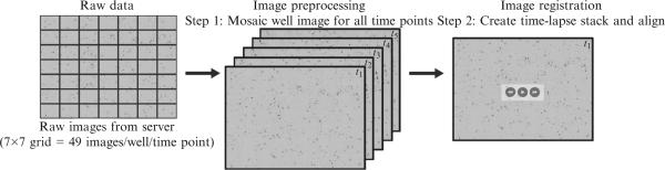
Workflow of image preprocessing and registration. Raw data (7 × 7 grid = 49 images) from each well are mosaiced to give a single image for each well at each time point. These images are then stacked together to make a time lapse. Each image in the time lapse is then registered to remove any hysteresis introduced from microscope stage movements.
1. Image preprocessing
The first stage of an analysis pipeline involves image preparation for subsequent analyses. It consists of assembling the acquired set of images into a larger mosaic image that is then processed for flattening uneven field illumination. These functions are performed by built-in filters available with most image analysis software. Some processes tend to alter signal information. We try to acquire high-quality images and work with raw data when doing intensity or similar measurements which would be altered by image processing (Fig. 17.3).
2. Image registration
The goal of an image registration algorithm, given two or more images from a time-lapse series, is to estimate a mapping that will bring the images into alignment. Each image in our time lapse is acquired ~12–24 h apart and typically contains 5–15 neurons. Difficulties in registration result from cells moving, dying, or changing in intensity between times, and additional shifts can be introduced by microscope stage hysteresis. This reduces the intensity and spatial overlap of the positive objects (cells) in adjacent frames. Small misalignments or hysteresis in the stage is easier for an image registration algorithm to rectify if changes in composition between each image in a sequence are modest and incremental: image registration methods are either intensity-based, feature-based, or some blend of both (see Hill et al., 2001, for a comprehensive overview). We register images with algorithms from a number of different image analysis programs. MultiStackReg, an ImageJ plugin that uses an iterative cross-correlation alignment method (Thevenaz et al., 1998), has proved most efficacious for us in a wide variety of image stacks. However, images that contain no, few, or many out-of-focus cells tend to fail registration.
3. Image segmentation
Once the image is preprocessed and registered, cells are recognized using various segmentation algorithms. Segmentation is partitioning of an image into sets of pixels (segments) that correspond to distinct objects. This part of the image analysis process is the most difficult and probably the most crucial step for the success of the analysis.
We follow each neuron throughout the assay period and use disappearance of the cell body as a surrogate for neuronal cell death in our longitudinal studies (Arrasate et al., 2004). To aid segmentation, we seed the cells at a low-medium density (~70,000 cells/well). Because primary neurons are difficult to transfect, the transfected cells are well dispersed, reducing segmentation errors. The first time point (~24 h posttransfection) shows dim cells because most FPs take 24–48 h to accumulate enough to achieve steady state levels that can be detected with our illumination setting and camera. By the second to third time points, intensities of most cells stabilize except for a few dim cells that show low or delayed expression and survival differences begin to emerge between different assay conditions. From the 3–4th frames onward, we look for further separation of survival trends to achieve statistical significance.
Such dynamic time-lapse images pose a significant challenge for an accurate segmentation, as it needs to be (1) flexible to handle changing cell intensities, shapes, and sizes; (2) specific to consistently select live cells; and (3) accurate to report the correct lifetime of each cell. In our experience, none of the generic segmentation algorithms from standard image analysis software were adequate. They either reported too many false positives, corrupting the analysis with the presence of nonexistent cells, or detected fewer cells than were present, causing subsequent analyses to be biased toward more clearly distinguishable cells. Thus, we developed a transiently transfected primary neuron segmentation algorithm using Image-Pro Plus.
We describe here one of our most commonly used HTS segmentation pipelines, which detects and tracks only cell bodies in time-lapse images (Fig. 17.4). We tend to use survival for primary screening. Our other segmentation approaches give more detailed morphological readouts during secondary and tertiary screening.
Figure 17.4.

Image segmentation, cell tracking, feature extraction, and data reporting. (A) Shows a typical montaged image showing the first time point after image segmentation. Unique cell track numbers are shown in red next to each cell. Two regions within this image have been zoomed in to show cell lifetime detection from the entire time lapse. (B) A typical delimited text file showing the arrangement of data output and feature extraction by the analysis program. (C) Shows a representative heat map of a control plate where a known modifier (blue outlined wells) was spotted throughout the plate in the midst of positive control wells (green outlined wells). White shaded wells indicate longer survival and dark red shaded wells indicate reduced survival. The numbers represent the cumulative death in each well at the end of the experiment. (D) A survival curve from a modifier well showing decreased hazard (increased survival) compared to the negative control wells. (See Color Insert.)
The pipeline uses a series of filters and operations. Since cell bodies and particulate debris show up as spots and neurites as elongated “thread-like” structures, we first use a spot locate filter to exclude the neurites. This filter consists of a mean-filter that “smoothes” the image by averaging the pixel intensities in a 9-pixel square (3 × 3), followed by a watershed transformation to separate spots from the background. This detects the cell bodies as they are usually larger than the scattered debris from dead cells. A top hat filter is then used to distinguish neurons from debris. The algorithm uses three parameters (i.e., top radius, brim radius, and height) to relate to the object's appearance. The “top” of the “hat” is set at the maximum expected spot radius. The brim radius is often taken to be the shortest expected distance to the neighboring spot. The height of the top above the brim is set to the minimum intensity that a spot must rise above its immediate background. For this, the spot intensity is the average within the top, and the immediate background intensity is the average within the brim. This averaging reduces noise by decreasing the variance in the estimation of a noisy object and its background and thus improves the robustness and this performance of this filter from removing cell debris. Some very dim objects in the images are hard to decipher as being cells or debris without seeing the next time point in the time-lapse stack. We decided to use a simple thresholding operation to eliminate these very dim signals. Intensity statistics are calculated for the entire image, and then dim cells and background are eliminated by selecting pixels with values in the top fifth percentile. This approach provides flexibility to researchers in designing their assays (like choosing from a variety of fluorophores and having flexible image acquisition of each time point within the time lapse) and improves the efficacy of the segmentation method across a wide range of assay conditions. Finally, to locate and count cells, we binarize the image, converting the cell bodies so they have a pixel intensity value equal to 1 and the background has a value equal to 0. The resulting black and white image is further processed so that each cell is identified as an independent object with its own numerical identifier (Fig. 17.4).
4. Cell tracking
Our longitudinal assays require us to follow individual neurons over time. Cell-tracking algorithms are designed to track each individual positive object (cell) by linking the corresponding object in successive frames of a time-lapse sequence and designating it as the same cell from the previous frame or a new cell. Optimal image registration and segmentation of the time-lapse stack are prerequisites for reliable cell tracking. Poor segmentation will cause the cell-tracking algorithm to yield nonsensical tracks in which tracks from correctly segmented cells in one frame are connected to different cells or falsely segmented cells (i.e., debris) in the next frame.
Cell-tracking algorithms can be categorized into three main types. The centroid cell-tracking algorithm calculates the center-of-mass (centroid) of the object of interest. It performs best when all objects move in exactly the same way between consecutive frames, relative to each other and irrespective of changes in their shapes and intensities. The Gaussian cell-tracking algorithm directly fits Gaussian curves to the intensity profile and performs best when the intensities of the objects are same between consecutive frames, even if their movement is random relative to each other. In our assays, each time-lapse sequence contains many neurons, and between successive images, cells normally move randomly (at very modest speeds), their intensities change, cells disappear (die), new cells show up (delayed expression), and cells move in and out of the image due to the limited field of view of the microscope (Fig. 17.4A). For us, the third type of cell-tracking algorithm, a cross-correlation algorithm, performed best. It compares an image to a matrix of pixels (user defined) of a successive image. The matrix is shifted relative to the image in 1-pixel increments. For each increment, a correlation value is calculated that describes how well the values in the matrix match those of the image, and the program determines the shift that yields the maximum correlation value. This algorithm is computationally more intensive than the other two and significantly slows the analysis, depending on the size of the matrix selected.
5. Feature extraction
Feature extraction computes numerical descriptors of objects identified by segmentation. Features are classified into either low-level features (e.g., area, location, perimeter, and intensity) that are extracted directly from the image or high-level features (e.g., shape, texture, and projections) that are computed from the low-level features. The end result of extraction is typically an extensive set of features, commonly called a feature vector, on a per-cell or whole-image basis. We use objects with unique identifiers from the segmented binary image as regions of interest to allow extraction of numerical descriptors for low-level features like cell location (x-, y-coordinates), maximum diameter (major axis), minimum diameter (minor axis), ratio of major to minor axis, size (area), surface area (perimeter), average intensity, and intensity variance for each cell. Based on these features, we compute descriptors for the high-level feature, such as cell viability (scored as live or dead), cell censored (moved out of the image field), cell lifetime, cell migration between time points, inclusion formation, and number of inclusions on a per-cell basis (Fig. 17.4B). These cell descriptors are exported as comma-separated values that can then be either viewed (with programs like Microsoft Excel) or advanced further into the data analysis pipeline.
4.1.2. Multiple levels of analyses
Depending on whether the data is from a handful of plates (small-scale biological assay) or from a HTS assay, we analyze the data at three different population levels: well-level, multiwell and plate-level, and multiplate level. We use Pipeline Pilot (Accelrys, San Diego, CA) to automate our workflow and visualize results for each type of analysis. At the root of the data, a well is considered an individual experiment and is composed of a population of neurons with a known condition. The software automatically builds well information from the designated user-defined plate format (test wells, positive control wells, and negative control wells; Fig. 17.4C and D). For multiwell and plate-level analysis, the software compares data across multiple wells on a plate. In this way, we can easily identify potential biases, for instance, edge effects, outlier wells, and general issues with cell health. Heat maps are very informative when assessing these types of plate-level effects and can easily identify wells of interest or control wells that have not passed quality control measures. For multiplate and experiment level analysis, the software collects data for replicate wells on different plates and is useful for increasing the sample size when the effect size is small. Furthermore, the full power of HCS datasets comes from mining a central database where data from hundreds to thousands of plates are stored. Existing datasets can be reanalyzed to answer new questions and meta-analyses can be carried out by pooling large amounts of data that have accumulated over many years.
4.2. Image analysis software packages used in our laboratory
HCS imaging platforms come equipped with software for image acquisition control, image analysis, statistical tools, data visualization tools, and a database for storing and retrieving data. These algorithms are adaptable to screening in different cell lines with different markers. They are meant to be used with minimal training and do not require the user to develop his own tools or to be able to program. Drawbacks of such ready-to-go systems are the source code is protected and the user does not know the methodology of the different steps, cannot modify them, or fully understand their functionality. Also, proprietary software licenses might not be affordable for all users. The existing platforms can be divided into two categories: open source and proprietary. Open source softwares used in our laboratory are ImageJ and CellProfiler, and the proprietary software includes MATLAB, Metamorph, Pipeline Pilot, and Image-Pro (Table 17.4).
Table 17.4.
Image analysis softwares used in our laboratory
| Open source | |
| CellProfiler | MATLAB-based open source image analysis package (compatible with Mac OS X, Windows, and Unix) for cellular HCS (Carpenter et al., 2006). Specifically designed to bridge the gap between developer tools, such as MATLAB and the proprietary software for HCS, and offers ~50 modules for typical image analysis steps with user-friendly GUIs. MATLAB is not required to run the application, but MATLAB users can access the source code, expand the capacities of the program with new code, and modify existing code to adapt to specific problems. It accepts many conventional image formats, and new ones can be encoded. A pipeline is created using the various modules to automate the analysis. CellProfiler is relatively new, but a user community is growing; so new modules may appear at an increasing rate. As CellProfiler was designed for HCS, distributed computing is feasible, so that clusters can be used. |
| ImageJ | Java-based open source image analysis package (compatible with Mac OS X, Windows, Unix, and Linux) has a large user community and over 300 plugins (modules). Plugins accept most image formats, and new ones can be coded in. Macros are created using the various plugins to automate the analysis. Our laboratory uses FIJI, an ImageJ distribution along with a plugin updater with a graphical user interface and many ofthe necessary plugins preinstalled and organized in a coherent structure. Using custom macros, we use the image registration capabilities of ImageJ and have also semiautomated image analysis for our autophagy, RNA granule tracking, and neuronal branching assays. |
| Commercial/proprietary | |
| MATLAB | Commercially available development environment (compatible with Mac OS X, Windows, Unix, and Linux) is widely used in engineering for a wide range ofapplications and can also be used for image analysis (with appropriate toolboxes). Although Matlab is proprietary, applications with Matlab languages are freely available (Cellprofiler (Carpenter et al., 2006), CellC (Selinummi et al., 2005)). It easily interfaces with other softwares and accepts most conventional image formats. As a developer tool, it is highly flexible but also requires time to optimize the image analysis process. It can handle distributed computing to enable clusters for parallel and faster analysis. |
| Image-Pro Plus | Commercially available image acquisition and analysis package (compatible with Windows only). It has multichannel and multiwell plate image acquisition formats. To give us more control and flexibility of our acquisition settings, we have written macros for automating the entire image acquisition process. We routinely use it for analyzing our HTS data. It accepts some common image formats and easily interfaces with other software. Some of our analysis pipeline is controlled by a simple Perl script that calls Image Pro plus at appropriate times and feeds in and out the appropriate images. It has options to link to databases to retrieve and store image data and has a moderate-sized user community. |
| Metamorph | Commercially available image acquisition and analysis package (compatible with Windows only). The modules are designed for biology-specific applications. It has multichannel and multiwell plate image acquisition formats. We routinely use it for image acquisition and to give us more control and flexibility of our acquisition settings, we have written journals for automating the entire image acquisition process. Also has a moderate-sized user community. |
| Pipeline pilot | Commercially available program for dataflow management, image analysis, and reporting that provides an easy way to build pipelines for customized data analysis (compatible with Windows only). It can read all standard and some proprietary file formats and has the advantage of being able to run ImageJ, Matlab, Python, and R scripts. Dataflow pipelines are created through sequential addition of drag-and-drop components acting at different points in the analysis. Data can be written in a variety of formats, including storage within databases or saved in delimited text files. Users can connect remotely to a Pipeline Pilot server through a web browser and process images with any saved pipeline. |
5. Statistical Approaches to HCS and Multivariate Data
The power of HCS datasets lies in the ability to parameterize cellular morphologies, intensities, and textures with multiple variables, allowing the identification of interesting phenotypes with minimal bias and greater sensitivity. Biases are minimized because rather than a priori deciding on a single feature that is thought to differ between two cell populations, many possible features and combinations of features are compared in parallel, and the most distinguishing features are statistically identified through variable reduction methods. Collinet et al. (2010) used multiparametric techniques to identify differences in endocytic uptake of two types of cargo. In a similar manner, Loo et al. (2007) determined differential response of cancer cells to drug treatment and could predict drug class and on- and off-target effects from the multiparametric signature. Support vector machine (SVM) algorithms were used to determine hyperplanes of maximal separation between cell populations in multivariate space, and SVM recursive feature elimination was used to reduce the number of variables. All algorithms were implemented in Matlab. These examples are some of the first to use multichannel, fluorescence datasets to quantify cellular phenotypes.
As described above, our lab extracts baseline characteristics in the form of a few variables from multichannel fluorescence images of neurons to determine their effect on future outcomes (e.g., htt IB formation or cell death). We track individual cells over time to capture dynamic changes and compare cell populations by Cox proportional hazards (CPH), a statistical model for determining the effects of multiple variables on time-to-event outcomes (Klein and Moeschberger, 2003). Analysis programs analyze the images and produce a delimited text file containing the variables and outcome measures (Fig. 17.4B). R (www.r-project.org), a comprehensive and widely adopted open source statistics program, then imports the file and a Cox model is fit to the data with the R survival package. The CPH model is created as follows:
Required R packages: splines and survival
# This code fits a CPH model to data from two constructs #to determine how the constructs
# effect neuron survival
# Load splines package
library(splines)
# Load survival package
library(survival)
# Create a color vector for plotting
Colrs < – palette()
# Import csv file into dataframe
exp.data < – read.csv(“NeuronSurvivalData.csv”);
# Create dataframe with only columns needed for building CPH model
# Assumes that “Lifetime”, “EventCensored”, and #“Condition” are column headings in the.csv file.
cox.data< –data.frame(time=exp.data$Lifetime, event=exp.data$EventCensored, group=as.factor(exp.data$Condition))
# Fit a Kaplan Meier model to the data and plot survival #curves.
km.model < – survfit(Surv(time,as.logical(event))~group,data = cox.data)
plot(km.model,main=”Kaplan Meier Curve for Survival”, xlab=”Time [hrs]”,col=colrs)
# Fit a CPH model based on Condition and Lifetime
cph.model < – coxph(Surv(time,as.logical(event)) ~group,data = cox.data)
cph.pval < – summary(cph.model)$coef[,5]
cph.HR < – summary(cph.model)$coefficients[,2]
# Print out a summary of the CPH model
summary(cph.model)
The standard test for determining if a particular low-throughput assay is amenable to HTS is calculation of the Z’-factor (Zhang et al., 1999). This number is calculated as a signal detection window between positive and negative controls scaled by the dynamic range. A Z’-factor >0.5 has historically indicated that there is a sufficient detection window for carrying out a screen. However, this factor was derived for biochemical assays, and because of the inherent higher variability of cell-based assays, laboratories now carry out screens where the Z’-factor is >0. We found that summarizing our time-dependent analysis with descriptive statistics (as used in the Z’-factor) did not capture the increase in sensitivity that is gained by tracking cells over their entire lifetime. We therefore chose to use statistical tests that are calculated from information contained in the entire survival curve. To estimate false-positive and false-negative hit rates, we use control plates with one column each of positive and negative controls and then spot known positive controls randomly throughout the test wells of the plate. We next compose CPH models for all the test wells and compute a hazard ratio between each individual well and the negative control column. p-Values are calculated from the hazard ratios, and if the well is significantly less toxic than the negative control column, we label the well as a hit. The decision to screen is based on acceptable positive and negative likelihood ratios (LR+ and LR–, respectively) that are computed from up to four replicate plates. The stringency of the test (i.e., the threshold of the p-value) can be used to adjust the rates of false positives and negatives. Typically, in primary screens, false negatives are worse than false positives because false positives will eventually fail in secondary screens, whereas false negatives are lost completely.
6. Future Directions
Embryonic stem (ES) cells and induced pluripotent stem (iPS) cells are other model systems with great potential for HCA–HTS neurological disease assays. Because human neurological diseases are the result of tens to hundreds of risk factors that jointly and in different combinations lead to a clinical phenotype, ES cells and iPS cells may more realistically model such multifactorial diseases than primary neurons from rodent tissues. Further, murine models contain thousands of small base-pair changes that differ between human cells. Thus, studying disease states in rodent tissues may miss key components of neuropathology.
Because iPS cells are derived from human tissues, they carry all of the associated endogenous genetic components, which will likely more accurately reflect the biology of human disease. They also combine the physiological relevance of primary cells with the ease of culturing of immortalized cell lines.
The discovery that human fibroblasts taken from patients’ with neurological disorders can be genetically reprogrammed into iPS cells (Takahashi and Yamanaka, 2006; Takahashi et al., 2007; Yu et al., 2007) and differentiated into neurons that can retain biochemical and pathological deficits observed in the actual disease (Ebert et al., 2009; Lee et al., 2009; Marchetto et al., 2010; Seibler et al., 2011) will revolutionize our ability to model neurodegenerative diseases in a culture dish. In addition, These findings have opened up possibility of screening for drug therapeutics in a disease-specific, “human-centric” platform. Thus, HCA–HTS assays could use patient-derived cell lines to model multifactorial neurological diseases and rapidly generate potential hits with very high therapeutic values.
Our lab is differentiating iPS cells into specific cell types affected in HD, such as MSNs (Aubry et al., 2009), motor neurons that are affected in amytrophic lateral sclerosis and spinal muscular atrophy (Ebert et al., 2009; Dimos et al., 2008) and dopaminergic neurons that are lost in Parkinson's disease (Seibler et al., 2011; Wernig et al., 2008). We optimized these differentiations to a 96-well format and are subjecting these specific cell-types to our automated imaging time-lapse microcopy to track cell death, neuron dynamics, and cellular morphologies such as neurite and process length over time. We are investigating phenotypes of iPS lines generated from patients with HD that would be suitable for screening purposes. Finally, we are generating new iPS cell lines from individuals with HD, Amyotrophic lateral sclerosis, and Parkinson's disease that will be used in our HCA–HTS. Our goals are to subject neurological disease-specific iPS cells to HCA–HTS to create more well-suited platforms for drug screening to identify much needed biotherapeutics for neurodegenerative disorders.
7. Concluding Remarks
Although other systems achieve higher throughput than the transiently transfected live primary neuron screening system we have described in this chapter, the assay has greater sensitivity than commercially available systems due to the longitudinal approach and the ability to follow individual neurons over long periods of time. This significantly reduces the need for a large number of cells to detect statistical significance in our assay. As the hardware and software technology for HTS progresses, we are striving to combine the consistent high-quality images with speed increases in automated image acquisition and analysis to potentially allow on-the-fly analysis of images that then informs the acquisition process.
Our current HTS assay is focused on measuring cell lifetime. However, multiple levels of information can be extracted, which requires the integration of information from a number of channels (such as bright field and fluorescence) and hundreds of cell attributes, such as size, shape, intensity, neurites, lifetime, or inclusion formation. This multiplexing improves the assay's relevance because the dataset allows much more sophistication in data and image analysis and interpretation of the cellular information. The successful development of such HCA–HTS primary neuron assays for neurodegenerative disorders promises more efficient identification of hits from a primary screen with high disease relevance and therapeutic–predictive value, thereby reducing extensive testing in a range of secondary assays.
ACKNOWLEDGMENTS
We thank members of the Finkbeiner laboratory for helpful discussions. K. Nelson provided administrative assistance, and G. Howard edited the manuscript. This work was supported by National Institutes of Health Grants 2R01 NS039746 and 2R01 NS045191 from the National Institute of Neurological Disorders and Stroke and by Grant 2P01 AG022074 from the National Institute on Aging, the J. David Gladstone Institutes, and the Taube–Koret Center for Huntington Disease Research (to S. F.); a California Institute for Regenerative Medicine (CIRM) fellowship Grant T2-00003 (to P. S); a CIRM fellowship Grant TG2-01160 (to J.K.); and the National Institutes of Health–National Institute of General Medical Sciences University of California, San Francisco Medical Scientist Training Program, (to A. D). The animal care facility was partly supported by a National Institutes of Health Extramural Research Facilities Improvement Project (C06 RR018928).
REFERENCES
- Arrasate M, Finkbeiner S. Automated microscope system for determining factors that predict neuronal fate. Proc. Natl. Acad. Sci. USA. 2005;102:3840–3845. doi: 10.1073/pnas.0409777102. [DOI] [PMC free article] [PubMed] [Google Scholar]
- Arrasate M, Mitra S, Schweitzer ES, Segal MR, Finkbeiner S. Inclusion body formation reduces levels of mutant huntingtin and the risk of neuronal death. Nature. 2004;431:805–810. doi: 10.1038/nature02998. [DOI] [PubMed] [Google Scholar]
- Aubry L, Peschanski M, Perrier AL. Human embryonic-stem-cell-derived striatal graft for Huntington's disease cell therapy. Med. Sci. (Paris) 2009;25:333–335. doi: 10.1051/medsci/2009254333. [DOI] [PubMed] [Google Scholar]
- Barmada SJ, Skibinski G, Korb E, Rao EJ, Wu JY, Finkbeiner S. Cytoplasmic mislocalization of TDP-43 is toxic to neurons and enhanced by a mutation associated with familial amyotrophic lateral sclerosis. J. Neurosci. 2010;30:639–649. doi: 10.1523/JNEUROSCI.4988-09.2010. [DOI] [PMC free article] [PubMed] [Google Scholar]
- Brouillet E, Conde F, Beal MF, Hantraye P. Replicating Huntington's disease phenotype in experimental animals. Prog. Neurobiol. 1999;59:427–468. doi: 10.1016/s0301-0082(99)00005-2. [DOI] [PubMed] [Google Scholar]
- Capenter AE, Jones TR, Lamprecht MR, Clarke C, Kang IH, Friman O, Guertin DA, Chang JH, Lindquist RA, Moffat J, Golland P, Sabatini DM. Cell Profiler: Image analysis software for identifying and quantifying cell phenotypes. Gen. Biol. 2006;7:R100. doi: 10.1186/gb-2006-7-10-r100. [DOI] [PMC free article] [PubMed] [Google Scholar]
- Collinet C, Stoter M, Bradshaw CR, Samusik N, Rink JC, Kenski D, Habermann B, Buchholz F, Henschel R, Mueller MS, Nagel WE, Fava E, et al. Systems survey of endocytosis by multiparametric image analysis. Nature. 2010;464:243–249. doi: 10.1038/nature08779. [DOI] [PubMed] [Google Scholar]
- Dalby B, Cates S, Harris A, Ohki EC, Tilkins ML, Price PJ, Ciccarone VC. Advanced transfection with Lipofectamine 2000 reagent: Primary neurons, siRNA, and high-throughput applications. Methods. 2004;33:95–103. doi: 10.1016/j.ymeth.2003.11.023. [DOI] [PubMed] [Google Scholar]
- Daub A, Sharma P, Finkbeiner S. High-content screening of primary neurons: Ready for prime time. Curr. Opin. Neurobiol. 2009;19:537–543. doi: 10.1016/j.conb.2009.10.002. [DOI] [PMC free article] [PubMed] [Google Scholar]
- Dimos JT, Rodolfa KT, Niakan KK, Weisenthal LM, Mitsumoto H, Chung W, Croft GF, Saphier G, Leibel R, Goland R, et al. ‘Induced pluripotent stem cells generated from patients with ALS can be differentiated into motor neurons’. Science. 2008;321(5893):1218–1221. doi: 10.1126/science.1158799. [DOI] [PubMed] [Google Scholar]
- Dudek H, Ghosh A, Greenberg ME. Calcium phosphate transfection of DNA into neurons in primary culture. Curr. Protoc. Neurosci. 2001:3.11.1–3.11.6. doi: 10.1002/0471142301.ns0311s03. [DOI] [PubMed] [Google Scholar]
- Ebert AD, Yu J, Rose FF, Jr., Mattis VB, Lorson CL, Thomson JA, Svendsen CN. Induced pluripotent stem cells from a spinal muscular atrophy patient. Nature. 2009;457:277–280. doi: 10.1038/nature07677. [DOI] [PMC free article] [PubMed] [Google Scholar]
- Finkbeiner S, Cuervo AM, Morimoto RI, Muchowski PJ. Disease-modifying pathways in neurodegeneration. J. Neurosci. 2006;26:10349–10357. doi: 10.1523/JNEUROSCI.3829-06.2006. [DOI] [PMC free article] [PubMed] [Google Scholar]
- Giepmans BN, Adams SR, Ellisman MH, Tsien RY. The fluorescent toolbox for assessing protein location and function. Science. 2006;312:217–224. doi: 10.1126/science.1124618. [DOI] [PubMed] [Google Scholar]
- Hertzberg RP, Pope AJ. High-throughput screening: New technology for the 21st century. Curr. Opin. Chem. Biol. 2000;4:445–451. doi: 10.1016/s1367-5931(00)00110-1. [DOI] [PubMed] [Google Scholar]
- Hill DL, Batchelor PG, Holden M, Hawkes DJ. Medical image registration. Phys. Med. Biol. 2001;46:R1–R45. doi: 10.1088/0031-9155/46/3/201. [DOI] [PubMed] [Google Scholar]
- Houston JB, Galetin A. Methods for predicting in vivo pharmacokinetics using data from in vitro assays. Curr. Drug Metab. 2008;9:940–951. doi: 10.2174/138920008786485164. [DOI] [PubMed] [Google Scholar]
- Inglese J, Johnson RL, Simeonov A, Xia MH, Zheng W, Austin CP, Auld DS. High-throughput screening assays for the identification of chemical probes. Nat. Chem. Biol. 2007;3:466–479. doi: 10.1038/nchembio.2007.17. [DOI] [PubMed] [Google Scholar]
- Klein JP, Moeschberger ML. Survival Analysis: Techniques for Censored and Truncated Data. 2nd edn. Springer; New York: 2003. [Google Scholar]
- Lavis LD. Histochemistry: Live and in color. J. Histochem. Cytochem. 2011;59:139–145. doi: 10.1369/0022155410395760. [DOI] [PMC free article] [PubMed] [Google Scholar]
- Lee H, Park J, Forget BG, Gaines P. Induced pluripotent stem cells in regenerative medicine: An argument for continued research on human embryonic stem cells. Regen. Med. 2009;4:759–769. doi: 10.2217/rme.09.46. [DOI] [PubMed] [Google Scholar]
- Linkert M, Rueden CT, Allan C, Burel JM, Moore W, Patterson A, Loranger B, Moore J, Neves C, Macdonald D, Tarkowska A, Sticco C, et al. Metadata matters: Access to image data in the real world. J. Cell Biol. 2010;189:777–782. doi: 10.1083/jcb.201004104. [DOI] [PMC free article] [PubMed] [Google Scholar]
- Loo LH, Wu LF, Altschuler SJ. Image-based multivariate profiling of drug responses from single cells. Nat. Methods. 2007;4:445–453. doi: 10.1038/nmeth1032. [DOI] [PubMed] [Google Scholar]
- Macarron R. Critical review of the role of HTS in drug discovery. Drug Discov. Today. 2006;11:277–279. doi: 10.1016/j.drudis.2006.02.001. [DOI] [PubMed] [Google Scholar]
- Macarron R, Hertzberg RP. Design and implementation of high-throughput screening assays. Methods Mol. Biol. 2009;565:1–32. doi: 10.1007/978-1-60327-258-2_1. [DOI] [PubMed] [Google Scholar]
- Marchetto MC, Carromeu C, Acab A, Yu D, Yeo GW, Mu Y, Chen G, Gage FH, Muotri AR. A model for neural development and treatment of Rett syndrome using human induced pluripotent stem cells. Cell. 2010;143:527–539. doi: 10.1016/j.cell.2010.10.016. [DOI] [PMC free article] [PubMed] [Google Scholar]
- Miller J, Arrasate M, Shaby BA, Mitra S, Masliah E, Finkbeiner S. Quantitative relationships between huntingtin levels, polyglutamine length, inclusion body formation, and neuronal death provide novel insight into Huntington's disease molecular pathogenesis. J. Neurosci. 2010;30:10541–10550. doi: 10.1523/JNEUROSCI.0146-10.2010. [DOI] [PMC free article] [PubMed] [Google Scholar]
- Mitra S, Tsvetkov AS, Finkbeiner S. Protein turnover and inclusion body formation. Autophagy. 2009;5:1037–1038. doi: 10.4161/auto.5.7.9291. [DOI] [PMC free article] [PubMed] [Google Scholar]
- Nolan GP. What's wrong with drug screening today. Nat. Chem. Biol. 2007;3:187–191. doi: 10.1038/nchembio0407-187. [DOI] [PubMed] [Google Scholar]
- Ohki EC, Tilkins ML, Ciccarone VC, Price PJ. Improving the transfection efficiency of post-mitotic neurons. J. Neurosci. Methods. 2001;112:95–99. doi: 10.1016/s0165-0270(01)00441-1. [DOI] [PubMed] [Google Scholar]
- Seibler P, Graziotto J, Jeong H, Simunovic F, Klein C, Krainc D. Mitochondrial Parkin recruitment is impaired in neurons derived from mutant PINK1 induced pluripotent stem cells. J. Neurosci. 2011;31:5970–5976. doi: 10.1523/JNEUROSCI.4441-10.2011. [DOI] [PMC free article] [PubMed] [Google Scholar]
- Selinummi J, Seppala J, Yli-Harja O, Puhakka JA. Software for quantification of labeled bacteria from digital microscope images by automated image analysis. Biotechniques. 2005;39(6):859–863. doi: 10.2144/000112018. [DOI] [PubMed] [Google Scholar]
- Spyropoulos DD, Bartel FO, Higuchi T, Deguchi T, Ogawa M, Watson DK. Marker-assisted study of genetic background and gene-targeted locus modifiers in lymphopoietic phenotypes. Anticancer Res. 2003;23:2015–2026. [PubMed] [Google Scholar]
- Staats J. Standardized nomenclature for inbred strains of mice: Eighth listing. Cancer Res. 1985;45:945–977. [PubMed] [Google Scholar]
- Takahashi K, Yamanaka S. Induction of pluripotent stem cells from mouse embryonic and adult fibroblast cultures by defined factors. Cell. 2006;126:663–676. doi: 10.1016/j.cell.2006.07.024. [DOI] [PubMed] [Google Scholar]
- Takahashi K, Tanabe K, Ohnuki M, Narita M, Ichisaka T, Tomoda K, Yamanaka S. Induction of pluripotent stem cells from adult human fibroblasts by defined factors. Cell. 2007;131:861–872. doi: 10.1016/j.cell.2007.11.019. [DOI] [PubMed] [Google Scholar]
- Thevenaz P, Ruttimann UE, Unser M. A pyramid approach to subpixel registration based on intensity. IEEE Trans. Image Process. 1998;7:27–41. doi: 10.1109/83.650848. [DOI] [PubMed] [Google Scholar]
- Tsvetkov AS, Miller J, Arrasate M, Wong JS, Pleiss MA, Finkbeiner S. A small-molecule scaffold induces autophagy in primary neurons and protects against toxicity in a Huntington disease model. Proc. Natl. Acad. Sci. USA. 2010;107:16982–16987. doi: 10.1073/pnas.1004498107. [DOI] [PMC free article] [PubMed] [Google Scholar]
- Wernig M, Zhao JP, Pruszak J, Hedlund E, Fu D, Soldner F, Broccoli V, Constantine-Paton M, Isacson O, Jaenisch R. Neurons derived from reprogrammed fibroblasts functionally integrate into the fetal brain and improve symptoms of rats with Parkinson's disease. Proc. Natl. Acad. Sci. USA. 2008;105:5856–5861. doi: 10.1073/pnas.0801677105. [DOI] [PMC free article] [PubMed] [Google Scholar]
- Yu J, Vodyanik MA, Smuga-Otto K, Antosiewicz-Bourget J, Frane JL, Tian S, Nie J, Jonsdottir GA, Ruotti V, Stewart R, Slukvin II, Thomson JA. Induced pluripotent stem cell lines derived from human somatic cells. Science. 2007;318:1917–1920. doi: 10.1126/science.1151526. [DOI] [PubMed] [Google Scholar]
- Zhang JH, Chung TD, Oldenburg KR. A simple statistical parameter for use in evaluation and validation of high throughput screening assays. J. Biomol. Screen. 1999;4:67–73. doi: 10.1177/108705719900400206. [DOI] [PubMed] [Google Scholar]
- Zhang JH, Chung TD, Oldenburg KR. Confirmation of primary active substances from high throughput screening of chemical and biological populations: A statistical approach and practical considerations. J. Comb. Chem. 2000;2:258–265. doi: 10.1021/cc9900706. [DOI] [PubMed] [Google Scholar]