Two-tone distortion in intracochlear pressure

Abstract

Two-tone distortion was measured in the intracochlear pressure in the base of the gerbil cochlea, close to the sensory tissue, where the local motions and forces of the organ of Corti can be detected. The measurements probe both the underlying nonlinear process that generates two-tone distortion, and the filtering and spreading of the distortion products. Some of our findings are as follows: (1) The observations were consistent with previous observations of two-tone distortion in BM motion [J. Neurophysiol. 77, 2385–2399 (1997); J. Neurophysiol. 78, 261–270 (1997)]. (2) Frequency sweeps show distortion product tuning and phase-versus-frequency behavior that is similar, but not identical, to single tone tuning. (3) The decay of distortion products with distance from the basilar membrane confirms the feasibility that they could drive the stapes by a direct fluid route, as proposed by Ren [Nat. Neurosci. 7, 333–334 (2004)]. (4) The phases of the distortion products within a single family (the group of distortion products generated by a single primary pair) in some cases alternated between 0° and 180° when referenced to the phases of the primaries. This behavior is predicted by a simple compressive nonlinearity.

I. INTRODUCTION

Normal cochlear operation relies upon cell-based forces that greatly boost the cochlea’s response at low-to-moderate stimulus levels. The cell-based forces are not linearly related to the stimulus and they introduce distortion into the cochlear response (reviewed in Ruggero, 1993). The response to a two-tone stimulus, in addition to the primary stimulus frequencies, contains frequency components at f₁–n(f₂–f₁) and f₂+n(f₂–f₁), where n is a positive integer. Other frequencies are also present in the response, but the f₁–, f₂+n(f₂–f₁) components form a prominent family of distortion components (distortion products, or DPs) that flank the primaries. Two-tone distortion has been measured and studied at many levels of the auditory system: perceptual (e.g., Goldstein, 1967; Zurek and Sachs, 1979), neural (e.g., Kim et al., 1980), in auditory emissions (e.g., Kemp, 1978; Probst et al., 1991) and in basilar membrane (BM) motion (Robles et al., 1997; Cooper and Rhode, 1997). Two-tone distortion in intracochlear pressure was measured close to the cochlear wall by Magnan et al. (1997) and Avan et al. (1998).

For a given two-tone combination, the distortion is produced within the region of the organ of Corti (OC) where the responses to the two tones overlap Smoorenburg, 1972; Kim et al., 1980; Siegel et al., 1982; Robles et al., 1997). The DPs, once present, will be filtered by the cochlea’s mechanics. Therefore, the local response at a particular DP frequency has been shaped by three processes: the cochlear-mechanical filtering of the primaries, the distortion generation process, and finally the cochlear–mechanical filtering of the DP.

This contribution examines two-tone distortion in the intracochlear pressure close to the BM. Measurements were made at a region that is tuned to ~20 kHz, in turn one of the gerbil cochlea. The experimental design and analysis were guided by two basic objectives: to better understand the underlying nonlinear process that generates the distortion, and to describe the spreading and filtering of the distortion products following their generation. Both these objectives were served with a stimulus protocol in which either f₂, f₁ or 2 f₁–f₂ were set at the BF of our sensor recording position. The localization of the generation process, and the longitudinal propagation of DPs were explored by measuring how the 2 f₁–f₂ and 2 f₂–f₁ DPs varied with the primary ratio and level. Vertical spreading was explored by measuring the decay of these DPs with the distance from the BM towards the cochlear wall. A second stimulus protocol, detailed frequency sweeps with a low f₂/ f₁ ratio, was used to measure the filtering of DPs. Finally, the nonlinear process underlying distortion generation was explored by analyzing the relative phases and magnitudes of components within DP families.

The pressure close to the BM is closely akin to BM motion. More concretely, fluid pressure gradients (spatial derivatives) are approximately proportional to fluid acceleration, and close to the BM, the fluid and BM are expected to move together. With single-tone stimuli, Olson (2001) used fluid pressure differences to derive BM velocity. The frequency tuning of the BM motion and of the fluid pressure close to the BM were similar to each other in the region of the BF peak and similar to BM motion tuning measured by others (reviewed in Robles and Ruggero, 2001). In line with this, the two-tone pressure responses measured close to the BM were similar to two-tone responses observed in BM motion (Robles et al., 1997; Cooper and Rhode, 1997). BM motion is closer than cochlear pressure to stereocilia motion, and BM motion measurements are more valuable than pressure measurements in that respect. However, measurements of pressure complement those of motion, and are able to probe particular aspects of cochlear mechanics that are not accessible with measurements of sensory tissue motion. For example, the spatial variation of DP pressure within the cochlea is useful for exploring how DPs get out of the cochlea to give rise to cochlear emissions, and the analysis of families of pressure DPs is useful for understanding the nonlinear force.

Several theoretical studies have explored the properties of the two-tone DPs that arise from a compressive nonlinearity [Engebretson and Eldredge, 1968; Fahey, 1989; Fahey et al., 2000; the series by Lukashkin et al. (1998, 1999, 2002)]. Similarly, in this contribution a simple nonlinear model is used to better understand the intracochlear distortion we measure.

Although we do not report here on cochlear emissions, the studies here are related to the study of emissions. Several direct experimental examinations of the link between emitted and introcochlear two-tone DPs (measured in intracochlear pressure or sensory tissue motion) have been performed (Magnan et al., 1997; Naryanan et al., 1998; Avan et al., 1998; Cooper and Shera, 2004; Ren, 2004).

II. METHODS

A brief description of methods is here; details have been published Olson, 1998, 2001).

A. Animal

The measurements were made in gerbils stimulated with one or two tones via a speaker coupled to the ear canal. Intracochlear pressure was measured by inserting specialized pressure sensors into the cochlear scalae through small holes that were hand-drilled through the bony wall of the cochlea. Pressure measurements in the scala tympani (ST) were made in the first turn of the cochlea where the BF was approximately 20 kHz. In ST the pressure was measured at a series of distances from the BM. The pressure in the scala vestibuli (SV) just next to the stapes was measured, either simultaneously with the ST measurement or after most of the ST data had been collected.

The animal was deeply anesthetized throughout the experiment and overdosed with anesthetic at the end of it. A tracheotomy was performed to maintain a patent airway. The animal core temperature was maintained at ~37 °C using a thermostatically controlled heating blanket. An electrode at the round window measured the compound action potential (CAP) response of the auditory nerve to tone pips, as a monitor of cochlear health Johnstone et al., 1979). The care and use of the animals were approved by the Institutional Animal Care and Use Committee of Columbia University.

B. Sensor

The pressure sensor consists of a glass capillary with inner and outer diameters 100 and 170 μm, tipped with a gold-coated polymer diaphragm. Light from a light-emitting diode is delivered via a fiber optic threaded into the capillary, and reflects from the diaphragm. The amount of light returning to the fiber optic for transmission to a photodetector varies linearly with the pressure-induced motion of the diaphragm Hu et al., 1992). As has been described previously, the sensors are calibrated individually by submerging them a known distance beneath the surface of a vial of water that is shaken with a known acceleration (Bruel and Kjaer model 4290). This produces a known pressure at the position of the sensor. The sensitivity of the sensors is approximately flat (within 3 or 4 dB) up to at least 40 kHz. The sensor sensitivity is usually ~−30 dB V/80 dB SPL, but it varies between usable sensors from ~−20 to −40 dB V/80 dB SPL. The noise level is set by shot noise in the photodetector at a level of ~−60 dB V; it depends on the quantity of light returning to the photodetector and also varies slightly with different sensors. In some cases the sensor stability was good with very little before/after experiment change, but changes of 6–10 dB were also common. The changes are due to the fragility and vulnerability of the sensitive membrane. The sensitivity changes are frequency independent—the sensitivity remains flat with frequency, just at a different level.

The presence of the sensor close to the BM might perturb cochlear mechanics. In Olson (2001) the perturbation was shown to be small but sometimes measurable, by producing small changes in the CAP response.

Sensor positioning in ST can influence the measurements. The sensor was aimed to face the basilar membrane based on extracochlear landmarks and the degree of actual centering varies among experiments.

Based on our evaluation, the sensors operate linearly and do not introduce distortion. The stiffness of the sensor in theory is primarily due to the stiffness of the air gap between the membrane and optic fiber, with a value of ~1 − 2 Pa/nm Olson, 1998). This stiffness is linear. Another stiffness, of similar size (theoretically slightly smaller) as the air gap stiffness, is the bending stiffness of the membrane. When driving at 80 dB SPL, the intracochlear pressure is ~110 dB, corresponding to ~6 Pa. This would produce ~3 − 6 nm motion of the sensitive membrane. The thickness of the membrane is ~1 μm, so the motion is a small fraction (~0.5%) of the membrane thickness. At extremely high stimulus levels (large enough to produce intracochlear pressures of 130 dB and above) the motion will be large enough that the membrane’s stiffness might begin to become nonlinear. [This nonlinearity is due to the geometry, not stretching the membrane material beyond its elastic limit (Timoshenko, 1959; Gummer et al., 1981).] Several observations rule out the membrane as producing the distortion measured here: (1) DPs could be measured even when one of the primaries was very small (which happened when a primary was nulled due to a slow-wave, fast-wave cancellation); (2) the size of the DPs decreased with the distance from the BM even when the primaries were in the fast-wave frequency region and did not decrease with distance; (3) in general, the DPs were larger close to the sensory tissue in the ST than they were in the SV, even when the primaries were of similar size in the two scalae. Figure 1 illustrates point (3). It shows the response in SV to two equal-intensity tones of 80 dB SPL in the ear canal. Any distortion is beneath the noise level, which is 60 dB beneath the level of the two tones. This specific case was taken from a cochlea that was not in excellent condition (based on the degree of compression in the single-tone responses and CAP thresholds) and these data do not reflect a general lack of measurable distortion in SV. The purpose of Fig. 1 is to illustrate the lack of mechanical distortion in the sensor and sound system.

FIG. 1.

Absence of system distortion. These data show the SV pressure response measured next to the stapes with two equal-intensity tones of 80 dB SPL delivered to the ear canal (f₁=22.2 kHz, f₂=24.5 kHz, f₂/f₁=1.1). This specific case was a cochlea (E2) that was not in excellent condition and these data do not reflect a general lack of measurable distortion in SV. The purpose of the figure is to illustrate the lack of mechanical distortion in the sensor and sound system.

C. Stimuli

Stimuli were single or two pure tones, 1–2 seconds in duration. Stimulation levels refer to the sound pressure level of each tone in the ear canal. Two-tone stimuli were generated digitally (TDT system II or III) and delivered via a closed system by a single Radio Shack tweeter. Two-tone DPs measured in a cavity were at least 70 dB less than the primaries when the primary level was 100 dB SPL.

The frequencies of the two tones were either swept from low to high with a fixed ratio, or were set so that f₁, f₂ or 2 f₁–f₂ was equal to the BF at the recording position, at different ratios. Figure 2 illustrates the stimulus pattern on the BM, showing a cartoon of a two-tone excitation pattern for a stimulus level of 50 dB SPL. The 2 f₁–f₂=BF condition is shown in the left panel, the f₁=BF condition in the middle and the f₂=BF condition on the right. Upper panels illustrate a small f₂/f₁ ratio (1.05), the lower panels a relatively large ratio (1.25). When the ratio is small, there is almost a complete overlap of the response to the two primary tones, and a substantial overlap of the DPs as well. At the ratio of 1.25, which is the highest ratio used, the overlap is much less. The basal overlapping region will be broader at higher stimulus levels. For example, Kim et al.’s (1980) Fig. 2 indicates a large degree of basal overlap at levels of 64 and 74 dB SPL.

FIG. 2.

Cartoon of a two-tone excitation pattern for frequencies around BF. A cartoon of the responses to single tones of frequency f₁, f₂ and two distortion component frequencies gives an idea of the degree of overlap of these excitation patterns, and their longitudinal position relative to the recording position. The patterns are shown for two different f₂/f₁ ratios. The excitation patterns of f₁ and f₂ are shown as solid lines, of 2 f₁–f₂ and 2 f₂–f₁ as dotted lines. The 2 f₁–f₂=BF condition is shown in the left panel, the f₁=BF in the middle and the f₂=BF condition on the right. Upper panels illustrate a small f₂/f₁ ratio (1.05), the lower panels a relatively large ratio (1.25). [Regarding the construction of the cartoon: The excitation patterns are based on single-tone frequency sweep data at a stimulus level of 50 dB SPL from animal W43, after smoothing and eliminating the fast-wave plateau. To transform the frequency response to a spatial excitation pattern we used the assumption (scaling symmetry) that the tuning Q of the BM is similar at different frequencies. We then generated a family of responses, with each member peaking at a different frequency and corresponding to a different longitudinal location along the cochlea. The longitudinal locations were determined using the place-frequency map of the gerbil cochlea (Muller, 1996). The family of response curves was used to read off the response to a single frequency at different longitudinal locations, generating the plot of response versus position, the “excitation pattern” of the response. This is a standard transformation used in cochlear models, e.g. Geisler and Cai (1996).]

D. Analytical methods

The pressure responses were time averaged and analyzed via Fourier transform offline using MATLAB.

A discussion of phase requires a suitable reference phase. For single-tone measurements, the phase reference is typically the phase of the stimulus: of stapes motion, or ear canal pressure or SV pressure close to the stapes, for example. However, the DP frequencies are not present in the stimulus and such a convenient reference does not exist. In many two-tone studies the stimulus is set so that the primary phases both=0° in the ear canal, and then the phase reference can be taken to be 0°. In our studies we either reference the DPs to the SV pressure measured near the stapes or to the local ST pressure. These primary phases generally are not 0°. In order to find a suitable reference phase for each DP we use some basic rules about nonlinear system responses. A brief mathematical interlude follows, which provides a background for understanding the phase reference.

The instantaneous nonlinear system response of an input signal of the form [A cos(a)+B cos(b)], where a and b have the form ωt+ϕ, (a, b=phases, ω=radial frequency, ϕ=phase offset), will output a waveform composed of components whose phases are combinations of the input phases. The particular combinations can be found by first expanding the nonlinear process in a power series. After the input signal is processed by the nonlinearity, the resultant output series is again expanded using cosine rules (Duifhuis, 1989). Following these two expansions a nonlinear process might be found to produce a component with a phase of, for example, 2a–b. The frequency of this component is 2ω_a–ω_b and the phase offset is 2ϕ_a–ϕ_b. The nonlinearity will produce DPs whose phase offsets, when referenced to the primary phase offsets in the same combination as the combination of primary frequencies in the DP frequency, are 0° (or 180° to allow for interpreting a DP coefficient with a negative sign via phase). (Usually the “phase offset” is referred to as the “phase,” and this convention is followed in the rest of the paper.) More discussion along these lines is in Weiss and Leong (1985), who analyzed the harmonic output of a compressive nonlinearity when the input was a pure tone.

Because this concept is important to the analysis of our data, we illustrate it with a simple model. Figure 3 shows the family of DPs produced by running a two-tone stimulus through an instantaneous compressive nonlinearity. The nonlinearity was conceived as a BM velocity-to-OHC force transducer, based on the results that in a macromechanical sense the active force has the character of a (negative) resistance (Kolston, 2000; de Boer and Nuttall, 2000; Shera, 2001), at least at frequencies close to the peak [Fig. 3(a))]. However, this aspect of the nonlinearity is not critical; the important aspect is that an input (which could be anything—displacement, velocity, current, voltage, etc.) gives rise to an instantaneous output (force, displacement, voltage, etc.) that scales compressively with the input. The functional form of the nonlinearity we use in our model is included in the figure. The output of the nonlinearity for a two-tone L₁=L₂ input is shown in Fig. 3(b) (time domain) and 3(c) (frequency domain amplitudes). In Fig. 3(d), the frequency domain phases of the DPs are plotted. The phases were referred to the phases of the output at the primary frequencies, in the combination as described above. (For example, the phase of the DP at the frequency of 3f₁–4f₂ was referenced to the phase 3ϕ₁–4ϕ₂.) The amplitude of the DP family forms a symmetric stair–step response. The phases are either 0° or 180° (0 or ±0.5 cycles) and in general the phase alternates between these two values. The precise functional form of the nonlinearity is not critical to these aspects of the output. For example, nonlinearities that more closely mimic the measured form of the OHC displacement-current transducer, or are steeper or shallower functions, give similar results. On the other hand, the pattern is not absolute: offsets in the nonlinear function can produce changes, for example, single DPs might be greatly reduced. Sometimes the neat alternation between 0° and 180° falters, as observed in Fig. 3. We will see the stair–step DPs in many of our results, similar to the distortion families shown in Robles et al. (1997). More complicated distortion families are typically seen in cochlear emissions (Kemp and Brown, 1983), likely because the whole cochlea participates in generating and propagating those. When L₁ or L₂ is increased in value, predictable changes in the stair–step pattern occur, based on the simple nonlinear system response Engebretson and Eldredge, 1968; Fahey et al., 2000). Most notably, an increase in L₂ is expected to cause decreases in the low-side DPs, and an increases in L₁ is expected to cause decreases in the high-side DPs. The size of the low-side DPs as L₁ becomes greater than L₂, and of the high-side DPs as L₂ becomes greater than L₁ can be an increase or a decrease, depending on the particular L₁, L₂ sizes with respect to the parameters of the nonlinearity. Offsets of the nonlinearity can lead to level-dependent notches (Fahey et al., 2000; Lukashkin et al., 2002).

FIG. 3.

Characteristics of two-tone distortion components produced by a simple compressive nonlinearity. (a) The nonlinear function is a simple compressive nonlinearity, offset to increase its generality and be more similar to OHC input–output curves (Kros et al., 1995). For illustrative purposes, the nonlinearity takes velocity as an input and outputs force, but these specific inputs and outputs are not important to the general results. The parameters used in the nonlinear function are exp=1/3, A=63 pN, v_w=1 μm/s, v₀=200 μm/s and A₀=370 pN. (b) The output of the nonlinearity in the time domain for a two-tone input with amplitudes L₁=L₂=1000 μm/s. (c) The same output in a frequency domain amplitude plot shows the characteristic stair–step response. The two-tone distortion products at frequencies f₁+n(f₂–f₁) (n an integer) are circled. (d) The frequency domain phases of the two-tone distortion products f₁+n(f₂–f₁) referred to the phases of the output at the primary frequencies in the combination ϕ₁+n(ϕ₂–ϕ₁). The phases, so referenced, are always 0° or 180° (i.e., 0 or 0.5 cycle.) Note that −0.5 and 0.5 cycle are the same phase.

In our experiment the input of the nonlinearity (perhaps stereocilia displacement?) is not accessible, and instead we use either the primary members of the local ST pressure DP family, or the SV primary pressures (measured near the stapes) to construct the reference. It is useful to consider these references: Define Φ_dt and Φ_dv as the phase of a DP measured in the ST pressure close to the BM and referenced to ST or SV pressure primaries. The DP will have frequency f₁+n(f₂–f₁), where n is a positive or negative integer. (n=the DP number, except n=0, n=1 correspond not to the DPs but the primaries and n=2 is the first high-side DP, 2 f₂–f₁. n=−1 is the first low-side DP, 2 f₁–f₂.) The referenced phase of each DP is found as

$${\Phi }_{\mathit{dt}\_n}={\varphi }_{\mathit{dt}\_n}-\{{\varphi }_{t1}+n({\varphi }_{t2}-{\varphi }_{t1}\left)\right\}\left(\mathrm{ST}\text{reference}\right),$$ (1)

$${\Phi }_{\mathit{dv}\_n}={\varphi }_{\mathit{dt}\_n}-\{{\varphi }_{v1}+n({\varphi }_{v2}-{\varphi }_{v1}\left)\right\}\left(\mathrm{SV}\text{reference}\right).$$ (2)

(ϕ_{dt_n} is the phase of the DP of number n measured close to the sensory tissue in ST, ϕ_t1 and ϕ_t2 are the phases of ST primaries 1 and 2, and ϕ_v1 and ϕ_v2 are the phases of SV primaries 1 and 2.)

The distortion referenced to the SV pressure at the stapes can be rewritten in terms of Φ_dt:

$${\Phi }_{\mathit{dv}\_n}={\Phi }_{\mathit{dt}\_n}+({\varphi }_{t1}-{\varphi }_{v1})+n\left\{\right({\varphi }_{t2}-{\varphi }_{v2})-({\varphi }_{t1}-{\varphi }_{v1}\left)\right\}.$$ (3)

The third term, n{(ϕ_t2–ϕ_v2)–(ϕ_t1–ϕ_v1)}, is equal to n times the difference in the traveling wave phase of the two primaries. This difference will be small for a low primary ratio, and in that case the third term will be small. Then the first two terms of the expression, Φ_{dv_n}=Φ_{dt_n}+(ϕ_t1–ϕ_v1), show that the phase of the distortion referenced to the SV phase can be interpreted as the phase of the distortion referenced to ST phase plus the single-tone traveling wave phase (ϕ_t1–ϕ_v1). The phase of the distortion referenced to ST phase will reflect the relationship between the ST pressure and the nonlinear force and will be influenced by whether the measured distortion was locally generated, or traveled from a more apical or basal location. What the data reveal about these relationships will be discussed below.

III. RESULTS AND DISCUSSION

Results from five animals (W34, W43, W45, E1 and W48) are shown in this contribution, and others showed similar results. In the experiments reported here the intracochlear pressure responses to pure tones in ST close to the BM were compressively nonlinear at frequencies close to the BF and the responses remained stable for several hours. The two-tone data from these preparations were consistent with each other, although not every dimension of the measurement (frequency sweep, variation with distance from BM, etc.) was made in every animal. The CAP thresholds of these animals were healthy following the initial surgery: ~30– 40 dB SPL at 20 kHz, ~20– 30 dB SPL at the most sensitive frequencies (~1 – 16 kHz) and increasing steeply for frequencies above 30 kHz. The shape of this CAP threshold tuning curve is similar to the behavioral threshold curve for a gerbil (Ryan, 1976) but elevated by ~20 dB, likely due to the different categories of measurement (Muller, 1996). Making the holes to the cochlea is the most invasive and potentially damaging step of the procedure and the experiments reported here were selected because this step was accomplished without substantial CAP threshold elevation. In several animals in order to minimize early damage the SV hole was not made until after most of the ST data had been collected. Then the SV hole was made and SV pressure close to the stapes measured, primarily to provide a phase reference. Thresholds in W43 and W48 were elevated by 5 dB at frequencies around 20 kHz after making the ST hole, and in W48 were elevated by 30 dB after several hours of experimentation with both ST and SV holes. Thresholds in E1 were elevated by 15 dB at frequencies around 20 kHz after making the ST and SV holes. Thresholds in W45 were not available after making the ST hole due to failure of the CAP electrode, but the single tone responses remained compressively nonlinear throughout the experiment.

A. Observations on single-tone responses

The responses to single-tone stimuli are described briefly below. These responses preface our description of two-tone responses by providing a review of the basic pressure response in healthy cochleae. Intracochlear pressure responses to single-tone stimuli are described in more detail in Olson (1998, 1999, 2001).

Figure 4(a) shows the spatial variations in the ST pressure close to the BM in response to 50 dB SPL stimuli (Animal W43). Spatial pressure variations are proportional to fluid acceleration. At frequencies close to the pressure peak, the large spatial variations in pressure (from one curve to the next) reflect the large fluid (and therefore BM) motions at these frequencies. At frequencies below the peak the pressure comes down, and the spatial variations are small. The large pressure value above the peak is due to the cochlear fast wave, and the very small spatial variations at frequencies above the peak reflect the small motions at those frequencies. As a brief review of the fast wave: when the stapes plunges in and out of the cochlea, the pressure difference in cochlear fluid between ST and SV vibrates the OC. The OC responds elastically, initiating the cochlear traveling wave—the “slow wave.” Because of the compressibility of the fluid, the excitation of the cochlea by the stapes also gives rise to a (much smaller) compressional fluid motion—a sound wave, known as the “fast-wave.” Peterson and Bogart (1950) discussed the fast and slow waves quantitatively in a one-dimensional (1-D) cochlear model. 2-D and 3-D models show that evanescent modes are also present. The evanescent modes are like the fast wave in being closely tied to the stapes motion but like the slow wave because they are associated with bulk, noncompressional fluid motion Steele and Taber, 1979; Watts, 2000). These modes are generally small.

FIG. 4.

Single-tone tuning characteristics in ST in the first turn of the gerbil cochlea (W43). (a), (b) ST pressure amplitude and phase (relative to the pressure in SV close to the stapes) with a stimulus level in the ear canal of 50 dB SPL, measured over the range of distances from the BM indicated in the legend. Spatial pressure variations indicate fluid motion. (c) (d) ST pressure measured 15 μm from the BM, with the stimulus level varying from 30 to 80 dB SPL in the ear canal. Pressure amplitude gain (ST pressure/ear canal pressure, expressed in dB) and phase relative to the SV pressure. The greatest total phase change in the pressure is roughly two cycles due to the domination of the fast-wave pressure at frequencies somewhat above the peak. The legend indicates the sound pressure levels in the ear canal. The pressure scales nonlinearly with stimulus level in the region of the peak.

Returning to the results of Fig. 4(a): close to the BM (within ~30 μm) at frequencies below and through the BF (~19 kHz), and more so at low stimulus levels, the slow wave is substantially larger than the fast wave and a frequency sweep traces out the familiar basal-turn tuning curve, amplitude, and phase, of the cochlear traveling wave (Robles and Ruggero, 2001). This is apparent in the 15 μm position of Fig. 4(a) at frequencies below 23 kHz. Somewhat above the BF (frequencies greater than ~22 kHz) the vibration is dominated by the fast wave, which is apparent in the plateau in both amplitude and phase. The spatial variations in pressure identify the frequency regions of relatively large fluid motion as beginning about an octave below the BF peak and ending about a quarter octave above it. Notches can arise due to fast-wave/slow-wave cancellation, most prominently in Fig. 4(a) at 16 kHz, 120 μm. The fluid pressures associated with the slow wave decrease as they spread into the cochlear fluid and the phase accumulation decreases with distance away from the sensory tissue, until it causes only a small ripple in the phase (~15 kHz region at 120, 160 μm positions) on the “background” fluid pressure of the fast wave. (Note that even close to the BM the pressure phase accumulates less in the pressure than it does in BM motion (Robles and Ruggero, 2001). The relatively small phase accumulation can be simply understood as being due to the relatively large fast-wave pressure, which dominates the traveling wave pressure at frequencies somewhat above the peak. Fast-wave pressure is comparable in size to slow-wave pressure, but fast-wave motion is much smaller than slow-wave motion.)

Figures 4(c) and 4(d) show a frequency sweep, amplitude gain (amplitude relative to stimulus level) and phase, in the same animal at a distance 15 μm from the BM and at stimulus levels between 30 and 80 dB. The amplitude gain close to the BF increased by 21 dB as the stimulus level decreased over this range. The boosting of the response at low levels is apparent in the region of the peak; at frequencies above and below the peak the response scaled linearly. Figure 5 shows frequency sweeps of the pressure in ST at 25 μm from the BM at different sound pressure levels from animal W45. [This figure is just like Figs. 4(c) and 4(d) in a different animal.] The gain of the cochlear amplifier is 18 dB between 50 and 90 dB SPL. Results from this animal and position are used to illustrate several of our two-tone observations.

FIG. 5.

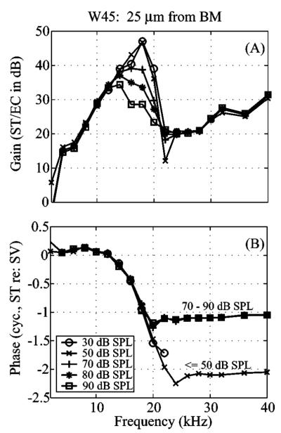
Single-tone tuning characteristics in ST in the first turn of the gerbil cochlea (W45, 25 μm from BM). ST pressure with stimulus levels of 30 to 90 dB SPL in the ear canal. Two-tone results from this animal are used to illustrate several of the studies. (a) Pressure amplitude gain relative to SPL in the ear canal. (b) Phase relative to the pressure responses in SV near the stapes.

B. Introduction to observations on two-tone distortion

Figure 6 introduces the two-tone pressure data, showing two-tone distortion measurements in the frequency domain. The results are from the 25 μm position of animal W45 at stimulus levels (L₁=L₂) of 60 and 80 dB SPL. The upper panels show results when f₂ and f₁ were chosen such that 2 f₁–f₂=BF (~18 kHz), the lower panels such that f₂=BF. The component at BF is circled. The level and number of DPs increased with the stimulus sound pressure level. A family of DPs was present with the smaller ratio, with the stair–step shape predicted in Fig. 3. The center-of-weight of the family shifted from the low side to the high side when the primaries shifted from a little above BF (2 f₁–f₂=BF) to a little below BF (f₂=BF) in frequency, indicating that the members of the DP family were subsequently filtered by the cochlea’s single-tone tuning. We will return to this in Fig. 9. With the larger ratio (1.15) only low-side DPs were present for the 2 f₁– f₂=BF condition, likely because the distortion was generated further basal (at the f₂, f₁ overlap region) and the high-side DPs were filtered from the recording position by the sharp high frequency cut-off of the cochlea’s single-tone tuning.

FIG. 6.

Two-tone pressure responses in ST in the frequency domain (W45, 25 μm from BM). The stimulus was two equal-intensity primary tones of 60 or 80 dB SPL in the ear canal. The upper panels show the results (amplitude of the response spectrum in dB SPL) when f₁ and f₂ were chosen such that 2 f₁–f₂=BF (~18 kHz), with f₂/f₁=1.05 (a), (b) and f₂/f₁=1.15 (c), (d). The lower panels show the results when f₂ was chosen such that f₂=BF, with f₂/f₁=1.05 (e), (f) and f₂/f₁=1.15 (g), (h). The component at BF is circled. With the low-ratio stimulus a stair–step distortion product family is observed, as predicted by the simple nonlinearity of Fig. 3. At the larger ratio relatively fewer distortion components are visible. For f₂/f₁=1.15 and 2 f₁–f₂=BF, it can be seen by referring to Figs. 4 and 5 that f₂ and f₁ are in the fast-wave dominated region where BM velocity (reflected in pressure gradients) is small while the “background” fast-wave pressure is large.

FIG. 9.

ST pressure DP families as frequency varies (W45, 25 μm from BM). A series of distortion families generated in response to L₁=L₂=80 dB SPL primaries of a range of frequencies. The f₂/f₁ ratio was fixed at 1.05 and the primary frequencies are indicated above the plots. An arrow indicates the 18 kHz BF in each plot.

The 2 f₁–f₂ response was a few dB greater than the f₁ response when it was at the BF [Fig. 6(c)], at the ratio of 1.15 and the stimulus level of 60 dB SPL. In the BM motion measurements of Robles et al. (1997) at a ratio of 1.25 and measuring at the 2 f₁–f₂ position, it was shown that the 2 f₁–f₂ DP could be present when f₂ was beneath the noise floor, and even when both f₂ and f₁ were beneath the noise floor. This was a conclusive observation that the DP was produced at a distant location and traveled to the measurement position. In our experiments, the background fast-wave pressure obscures such an observation. The primary frequencies at the ratio of 1.15 are 21 kHz and 24.4 kHz. The single-tone results of Fig. 5 illustrate that these frequencies were above the peak, in the fast-wave frequency region.

It is interesting to consider what the motion responses (or pressure response without the background fast wave) are in the time domain: A two-tone stimulus produces an amplitude-modulated beating pattern, with the envelope at the difference frequency, f₂–f₁. When the upper primary tone is well above the local BF, the beating envelope of the motion response would not be maintained in a linear cochlea, because only the lower frequency primary would be present in the motion. In contrast, in a healthy, nonlinear cochlea, because of the large 2 f₁–f₂ DP, the beating envelope would be maintained farther down the cochlea. A chain of nonlinear interactions might keep the envelope going. [For that matter, the f₂–f₁ component itself can be present in the nonlinear mechanical response (Kim et al., 1980; Cooper and Rhode, 1997.)]

The observations shown here and below use stimulus levels of 60–90 dB SPL. Although these levels are relatively high, the two-tone distortion measured is nevertheless attributed to nonlinearity in the cochlea’s active OHC force. To verify the physiological basis of the two-tone distortion, we measured it pre- and post-mortem in ST pressure close to the BM, at a stimulus level of L₁=L₂=80 dB. We found that DPs that were 30 dB out of the noise just pre-mortem had dropped below the noise level one half hour post-mortem. Avan et al. (2003) and Lukashkin et al. (2002) have argued that high and low level distortion likely arises from the same source. The studies by Avan et al. as well as studies reviewed in Kiang et al. (1986), and others, have identified the OHC as the source of cochlear nonlinearity. Referring to the single-tone data of Figs. 4 and 5, the response is compressive over the 60–80 or 90 dB SPL stimulus levels. In a compressively nonlinear cochlea at very high stimulus levels the response at the primary frequencies scales almost linearly. However, this does not mean that the response is “linear” at those levels, since distortion caused by the saturation of the nonlinear force will still be present. The relatively high-stimulus-level distortion is emphasized here simply because the whole family of DPs could be studied; at stimulus levels below 60 dB sometimes only the 2 f₁–f₂ DP emerged from the noise, and below 50 dB even it could not be detected. Two-tone distortion in BM motion was detectable at lower stimulus levels (Robles et al., 1997; Cooper and Rhode, 1997), most certainly due to a lower noise floor.

Several characteristics of the two-tone distortion are illustrated and discussed in the sections that follow. We show variations with distance from the BM (illustrated in Fig. 7), variations with primary ratio (Fig. 8) and DP tuning (Figs. 9–12). Finally, in Fig. 13 we return to individual distortion families to discuss the DP phase.

FIG. 7.

Spatial variations of ST pressure primaries and DPs (W34, E1). f₁, f₂ and the 2 f₁–f₂ and 2 f₂–f₁ DPs are shown as a function of distance from the BM. Results from two animals are shown; E1 , with BF 21 kHz, is labeled with subscript i and W34, with BF 18 kHz, is labeled with subscript ii. Dashed lines indicate the noise floor. Both of the primaries were set at 80 dB SPL, with f₂/f₁=1.1 for E1 and f₂/f₁=1.05 for W34. The upper panels (a)–(c) show the pressure amplitudes, the middle panels (d)–(f) show the phasenot referenced to anything—only the changes with distance are meaningful) and the lower panels (g)–(i) show the fluid velocity amplitude (the component in the direction perpendicular to the pressure sensor’s approach) derived from the amplitude and phase data. Within each three panel set the primary frequencies are varied such that 2 f₁–f₂=BF (a), (d), (g), f₁=BF (b), (e), (h) and f₂=BF (c), (f), (i). The pressure primaries, but not the pressure DPs, exhibit plateaus and notches in amplitude that are attributed to the fast-wave and fast-wave/slow-wave cancellation. The fluid velocities of the primaries and the fluid velocities of the DPs fall-off similarly with distance from the BM.

FIG. 8.

Dependence of ST pressure DPs 2 f₁–f₂ and 2 f₂–f₁ on primary frequencies and f₂/f₁ ratio (W45, 25 μm from BM). L₁=L₂ (solid lines) and L₁=L₂+10 (dotted lines) were the stimulus levels used, with L₂=60, 70 and 80 dB SPL. The upper panels show the pressure response at 2 f₁–f₂; the lower panels show the response at 2 f₂–f₁. The ratio is on the x axis of these plots and DP amplitude (in dB SPL) is on the y axis except for the far right panels, which plot the DP phase. The left panels show the case in which 2 f₁–f₂ was at the BF (18 kHz). To the right of those is the case in which f₁=BF, and then the case in which f₂=BF. The phase plots on the right also correspond to the case f₂=BF. (The phase is referenced to the ST pressure primaries. Only the f₂=BF phases are shown as then both primaries are slow-wave dominated, which is necessary to make this referencing meaningful.) In order to emphasize the influence of the DP frequency on the trends we find, the DP frequency, 2 f₁–f₂ or 2 f₂–f₁ is indicated on a secondary axis in the center of the plot. For the case in which 2 f₁–f₂=BF, the f₂ frequency is indicated on this axis.

FIG. 12.

Distortion product tuning in ST with equal-intensity two-tone stimulus (W48, 10 μm from BM). The primary tone levels were both 80 dB SPL with a fixed frequency ratio of 1.05. These data were from animal W48, with BF ~21 kHz, and were recorded at a distance 10 μm from the BM. The upper panels show how the amplitude (dB SPL) of 3 f₂–2 f₁, 2 f₂–f₁, 2 f₁–f₂ and 3 f₁–2 f₂ vary with frequency. Each DP is plotted versus its own frequency. Single tone tuning at 50 and 60 dB SPL are shown (dotted–dash lines) for a comparison. The middle panels show the DP phases relative to the SV primaries. The bottom panels show the DP phases relative to the ST primaries.

FIG. 13.

DP family amplitudes and phases (W45, 25 μm from BM). A two-tone stimulus with L₁=L₂=80 dB SPL and f₂/f₁ ratio=1.05 generated a family of DPs, as shown in the upper panels. The primary frequencies were such that 2 f₁–f₂=BF (left panels), f₁=BF (middle), and f₂=BF (right). The DP phases, referenced to the primary phases, are presented in the lower panels as crosses. The phases basically alternate in phase between 0° and 180° degrees, with sometimes a superimposed slope. In order to better visualize the slope, the phases that alternated by 180° have been also plotted as empty circles, with 180° subtracted or added.

C. Two-tone distortion: Variations with distance from the BM

Two-tone distortion is produced in the organ of Corti. The resulting distorted motion of the BM will produce fluid motions that spread into the cochlear fluid. Like the pressure field close to a speaker, this pressure disturbance will have a near-field and a far-field component, with the distance at which the near-field dominates ~ the dimension of the source. Figure 7 shows how the ST primary and 2 f₁–f₂ and 2 f₂–f₁ DP amplitude [Figs. 7(a)–7(c)] and phase [Figs. 7(d)–7(e)] vary with distance from the BM. Measurements were made approximately every 20 μm up to a 200 μm depth. Results from two animals are shown in Fig. 7, and are designated by the subscripts i (E1) and ii (W34). Figures 7(g)–7(i) use these results to find how the fluid velocity varies with distance from the BM. Fluid velocity was calculated from pairs of pressure measurements at adjacent positions as v_fluid≈ (i/ωρ)▽p where ω is the angular frequency and ρ is the fluid density Olson, 1998). The results shown are with an equal-intensity stimulus level of 80 dB SPL, and results at 60 dB SPL were similar. The primary ratio was 1.1 for animal E1 and 1.05 for animal W34. Within each three panel set [e.g., Figs. 7(a)–7(c)], the left panel corresponds to stimulus conditions such that 2 f₁–f₂ is equal to the BF of the recording position (where BF was chosen based on the low-stimulus-level single-tone responses), the middle panel corresponds to stimulus conditions such that f₁=BF and the right panel corresponds to stimulus conditions such that f₂=BF. Several aspects of these data are notable. Most obvious is that the primaries fall off less rapidly than the DPs. In general, both DPs drop steadily, in some cases reaching the noise level, whereas the primaries level off. The level off in the primaries is due to the background cochlear fast-wave pressure that basically fills the cochlea, as discussed above. Bii and Cii show a 20 dB notch in the response of one of the primaries, presumably due to a fast-wave/slow-wave cancellation. The DPs were unperturbed by the notches that occurred in the primaries. This immunity is reassuring, as it confirms that the distortion was not generated by the pressure sensor.

We were interested in using the variations in fluid pressure and fluid velocity amplitude with depth to explore the hypothesis that the 2 f₂–f₁ DP would decay differently with distance from the BM than the 2 f₁–f₂ DP. This hypothesis was based on the idea that 2 f₁–f₂ is generated in a part of the cochlea where it is able to produce its own traveling wave, whereas the 2 f₂–f₁ DP is generated in a region slightly apical of its own BF place, and would therefore be a nonpropagating disturbance. A nonpropagating disturbance might be expected to decay with distance differently than a traveling wave disturbance. As a background to this expectation: In 2-D models of the cochlea the penetration (decay) depth of the wave in the fluid is proportional to wavelength (de Boer, 1984). However, the results from a previous study Olson, 1999) showed that the 2-D model penetration prediction was not borne out for the response to single tones. In that study the penetration depth was found to be approximately equal for tone frequencies corresponding to a wide range of traveling wave wavelength. The interpretation of those results was that the decay with depth was influenced more by the finite width of the BM than by the wavelength. If the width is the governing feature of penetration depth, then the penetration of DPs and primaries might be able to identify a multimodal BM motion. Investigations of BM motion have shown that the electrically evoked BM motion is bimodal across the width of the BM (Xue et al., 1995; Nuttal et al., 1999). In contrast, the response to single-tone acoustic stimulation has usually been found to be unimodal across the width of the BM Cooper, 2000; Rhode and Recio, 2000), with the exception being the near-BF results of Nilsen and Russell (1999). The active force that gives rise to DPs might, like the electrically elicited motion, produce a bimodal disturbance across the BM. In the same way that the pressure decays more rapidly from a dipole source than from a monopole source (Beranek, 1993), the decay from a bimodal disturbance would be more rapid than from a unimodal disturbance. A DP that is based on a bimodal disturbance that does not propagate (high-frequency-side DP) would be expected to decay more rapidly in the fluid than components that launch or are associated with a traveling wave (the primaries and low-frequency-side DPs). The fluid velocity [Figs. 7(g)– 7(i)] is more useful than pressure for this comparison since the fast wave is effectively canceled out when taking the pressure differences to find fluid velocity; then the primaries can be included in the comparison. In general, the 2 f₁–f₂, 2 f₂–f₁, and f₁ and f₂ components all have a similar falloff in fluid velocity [Figs. 7(g)–7(i), i and ii]. The similar decays of primary and high- and low-side DP velocity reported here support the idea that the width of the BM is the governing dimension for penetration, and does not give any indication that these different components have different mode shapes.

The phase data plotted in Fig. 7 are not referenced to anything so only the variations with distance are meaningful, not the absolute values. [Elsewhere in this paper the DP phases are referenced to either ST or SV primary phases. For this figure, it made more sense to plot the unreferenced phase and concentrate on variations with distance because the stimuli (f₁, f₂, their phases) were identical for all the data within a panel.] The primary components change smoothly, and little, except in the region of a notch [ii of Figs. 7(e) and 7(f)] where expected 180° interference jumps are observed. All the DPs have a gradual phase increase with distance that can be as large as 1/3 of a cycle, 120°, over the 200 micrometers of measurement. In a 2-D, short-wave cochlear model, phase variation with depth is related to an amplitude decrease or increase in the direction of wave travel. [See the discussion of the solution to Laplace’s equation (▽²p=0) in a 2-D fluid in de Boer, 1984.] However, given the inability of the 2-D model to predict amplitude variations, a 3-D model is probably also required to interpret the phase.

The decay-with-depth of DP pressure is related to the question of whether the distortion reaches the stapes through the fluid pressure (as opposed to/in addition to a reverse traveling wave on the OC) to generate emissions. The DPs decay steadily over the 200 micrometers in depth that they were measured, to become pressures that are 20–30 dB smaller than they were close to the BM. At this point, the distortions were in some cases dropping beneath the noise level of our system at ~50 dB SPL (2 f₂–f₁ in Figs. 7(a)i and 7(c)i), although in other cases they are at ~ a 70 dB SPL level [2 f₁–f₂ in all panels but ii of Fig. 7(a)]. The stapes is about 1 mm distant from the recording position. Extrapolating the data of Fig. 7, the emissions will be reduced at least another 20–30 dB over a distance of 1 mm, to levels of ~20– 50 dB SPL. Reverse transmission through the gerbil middle ear probably produces about 20–30 dB of attenuation. This is based on measurements in a guinea pig (Magnan et al., 1997), and the ~30 dB gain of forward transmission Olson, 1998). Therefore, it is feasible that the distortion pressure would be large enough at the stapes to generate measurable emissions by this route. Studies by Ren (2004) showed a fast stimulation of the stapes by the 2 f₁–f₂ DP, presumably through the fluid pressure. Further work is required to understand the relative contributions of the direct fluid route and reverse-traveling-wave route to cochlear emissions.

D. Two-tone distortion: Variations with primary ratio around BF

Figure 8 shows the DPs as a function of ratio of the primaries. Results from W45 are shown, at a distance 25 μm from the BM. L₁=L₂ and L₁=L₂+10 were the stimulus levels used, with L₂=60, 70 and 80 dB. The ratio is on the x axis of these plots, and the DP amplitude (in dB SPL) is on the y axis, except for the far right panels, which plot the DP phase (relative to the primaries measured in ST) for the f₂=BF stimulus condition. The left panels show the case in which 2 f₁–f₂ was at the BF (18 kHz). To the right of those is the case in which f₁=BF, and then the case in which f₂=BF. The upper panels show 2 f₁–f₂; the lower panels show 2 f₂–f₁. Referring to Fig. 2, as the ratio increases, the region of primary overlap decreases. The distance between the DP best places and the overlap position also increases. In order to clarify the relationship between the BF and the frequencies at play, the DP frequency, 2 f₁–f₂ or 2 f₂–f₁, corresponding to the ratios, are indicated in the center of the plot. For the case where 2 f₁–f₂=BF, the f₂ frequency is indicated on this axis.

1. 2 f₁–f₂=BF (left column). The high-side, 2 f₂–f₁ DP (lower panel) decreased very rapidly with an increase in ratio. Compared to the 2 f₂–f₁ DP, the amplitude of 2 f₁–f₂ (upper panel) decreased much less rapidly with an increase in ratio. However, at the lowest stimulus level (60 dB), this DP did decrease rapidly for ratios above 1.15. This decrease and its level dependence agree with results of other investigators Cooper and Rhode, 1997; Robles et al., 1997). The effect of raising L₁ level so that L₁=L₂+10 was a general decrease of the high side 2 f₂–f₁ DP. This is the expected behavior of the nonlinearity, following the discussion of Fig. 3.

   The rapid decline in the high-side DP with increasing ratio is likely due to the combined effects of decreasing overlap region and single-tone filtering. The 2 f₂–f₁ DP’s best-place was basal to the cut-off frequency of the recording location, increasingly so as the ratio increased. The gradual decline in 2 f₁–f₂ with ratio can only be due to the decrease in the overlap region because, in contrast to the 2 f₂–f₁ DP, the 2 f₁–f₂ DP’s best place was at the recording position.

2. f₂=BF (right two columns). In this case the observation place was approximately at the distortion generation site, assuming that the generation site is where f₁ and f₂ responses spatially overlap and are both large. The 2 f₂–f₁ DP decreased slowly with the increase in ratio. The amplitude of the 2 f₁–f₂ DP had a zig–zag shape as the ratio increased. The 2 f₂–f₁ phase changed little with ratio compared with the 2 f₁–f₂ phase, which changed smoothly by almost a cycle as ratio increased from 1.05 to 1.25. When L₁ was increased so that L₁=L₂+10 dB, the high-side DP decreased as expected, following the discussion of Fig. 3. Another effect of raising the level of L₁ was that the high-side DP became almost unchanging with ratio. The low side 2 f₁–f₂ DP increased when L₁ increased. Its zig–zag shape was diminished, being replaced by a gradual decline with ratio, and the phase flattened out.

   2 f₂–f₁ is expected to be mainly a nonpropagating disturbance because its best place is basal to the recording position. In contrast, once generated, the 2 f₁–f₂ can travel apically towards its own best place. The measured 2 f₁–f₂ could be a summation of the local nonlinear generator component and a reflection component from close to the 2 f₁–f₂ best place (Brown et al., 1996; Talmadge et al., 1999). In line with this, the zig–zag amplitude variation of 2 f₁–f₂ with ratio is suggestive of interference. In this conceptual framework, the “smoothing” effect (on the amplitude and phase of the 2 f₁–f₂ DP) of raising the L₁ level relative to L₂ suggests that the generator component dominated the reflection component under those stimulus conditions (Mauermann and Kollmeier, 2004). The increasing phase with ratio for the L₁=L₂ condition reinforces the idea that the 2 f₁–f₂ DP is in part arising from a distant location. As Fig. 3 showed, a phase of a half cycle is expected for both the 2 f₁–f₂ and 2 f₂–f₁ DPs, at the output of a simple nonlinearity. The phase of the 2 f₁–f₂ DP gradually departed from the half cycle phase as the ratio is increased. This gradual departure might be due to the DP, or some fraction of it, being nonlocally generated. This might be the reflection component of the distortion, from the region of the 2 f₁–f₂ best place. The 2 f₂–f₁ DPs do not depart from the half cycle phase very much as the ratio is increased, suggesting that this distortion was dominated by a local nonlinear generator component.

3. f₁=BF (second column from the left). In this case the observation place was between the f₂ best place and the 2 f₁–f₂ best place. At the low ratio of 1.05, the amplitudes of 2 f₁–f₂ and 2 f₂–f₁ were nearly the same. At the higher ratio the 2 f₂–f₁ DP dropped off rapidly, but not as rapidly as when 2 f₁–f₂ was at BF. The 2 f₁–f₂ DP actually increased with ratio (L₁=L₂ condition) when the ratio increased from 1.05 to 1.1 but then decreased steadily. For L₁=L₂+10 dB, the high-side DP again had the expected general decrease, and the low-side DP’s most significant change was that it changed to monotonically decreasing with increase in ratio.

Considering all three recording conditions (BF= f₁, f₂ or 2 f₁–f₂) the 2 f₂–f₁ DP in general decreased with ratio. This is probably mostly due to the fact that its frequency was above the local BF, increasingly so as the ratio increased. The decreasing overlap region might also play a role, although this seems to be relatively minor, based on the very gradual decline with ratio in the f₂=BF case. At lower SPL, overlap effects would likely be greater. The 2 f₁–f₂ DP did not drop with ratio (at least up to f₂/f₁=1.25) for the f₂=BF condition. Both the f₂=BF and f₁=BF conditions showed nonmonotonic changes with ratio. High-side suppression of the DP by f₁ might account for the reduced size of the 2 f₁–f₂ DP at the lowest ratio in the f₁=BF condition Cooper and Rhode, 1997), but high-side suppression cannot account for the zig–zag pattern of the f₂=BF case. This behavior is more easily explained by interference between different components (nonlinear generator and reflection) of the 2 f₁–f₂ DP (e.g., Talmadge et al., 1999).

E. Two-tone distortion: Frequency sweeps at fixed ratio

Figures 9–12 show two-tone frequency sweep responses measured close to the BM at a ratio of 1.05 (animals W45 and W48). Figure 2 shows that the responses to the two primaries overlap a great deal with such a low ratio. As the primary frequencies are swept, this tightly overlapping pattern sweeps from apical to basal of the recording site. Figure 9 shows a series of distortion families in response to L₁=L₂=80 dB SPL primaries, at the frequencies indicated above the plots (W45, 25 μm from BM). The BF was ~18 kHz, indicated by an arrow in the plots. The characteristics of the distortion families are governed by both the local nonlinear response (which in general will produce stair–steps of DPs on either side of the primaries) and the single-tone tuning of both the primaries and the DPs. As the primaries sweep closer to the BF frequency the families of DPs grow. The influence of single-tone tuning of the DPs can be seen by comparing Fig. 9(c), whose primaries are just below the BF, to Fig. 9(d), whose primaries are just above the BF. The distortion family is weighted towards the high side in Fig. 9(c), towards the low-side in Fig. 9(d). [For completeness, the low-frequency primary is slightly bigger than the high-frequency primary in Fig. 9(d), which would also tend to shift the weight of the distortion family to the low side in this case.] Figure 9(e), with primaries even farther above the BF, shows a strong influence of single-tone tuning of the DPs. The center-of-mass of the distortion family is shifted left from the primaries, and is centered on the 18 kHz BF. The stair–steps shaping around the primaries is still apparent, however, in that the 2 f₁–f₂ DP is relatively large even though it is well above the BF. Referring to Fig. 5, the primaries in Fig. 9(e) are in the fast-wave dominant region; the slow-wave portions of the responses are expected to be small. It is likely that the whole DP family of Fig. 9(e) was generated basal to the recording position, where the slow-wave primary responses were large, with a primary-centered stair–step shape. Traveling to the recording position, the DP family was filtered by single-tone tuning, and arrived with the observed up–down–up shape. At lower frequencies the family of DPs is relatively less orderly [Figs. 9(a) and 9(b)] perhaps due to interference between locally generated and apically generated distortion. Although the primary frequencies in these panels would peak well apical of the recording site, the harmonic distortion in evidence indicates that some amount of nonlinear distortion was produced locally at these frequencies Olson, 2004).

Figures 10–12 plot the amplitudes and phases of responses such as those in Fig. 9, sorted by DP. The DPs are plotted relative to their own frequencies. Figure 10 shows data from animal W45 (25 μm from BM), ratio=1.05, and levels (L₁=L₂) of 60, 70 and 80 dB SPL. Fig. 11 is similar with L₁=L₂+10. Figure 12 shows results from another animal (W48, 10 μm from BM), ratio 1.05, L₁=L₂=80. The single-tone primary responses are also included as a reference, at levels of 30, 50 and 70 dB for W45 and 50 and 60 for W48. The tuning of the single-tones reflects the basic cochlear mechanical filtering.

FIG. 10.

Distortion product tuning in ST with equal-intensity two-tone stimulus (W45, 25 μm from BM). The stimulus tone levels were both either 60 (circles), 70 (crosses) or 80 dB SPL (pluses) with a fixed frequency ratio of 1.05. The upper panels show how the amplitude (dB SPL) of 3 f₂–2 f₁, 2 f₂–f₁, 2 f₁–f₂ and 3 f₁–2 f₂ vary with frequency. Each DP is plotted versus its own frequency. Single-tone tuning at 30, 50 and 70 dB SPL are shown (dotted-dashed lines) for a comparison. The middle panels show the DP phases relative to the SV primaries. The bottom panels show the DP phases relative to the ST primaries.

FIG. 11.

Distortion product tuning in ST with unequal-intensity two-tone stimulus (W45, 25 μm from BM). As in Fig. 10 except L₁=L₂+10 dB. The 3 f₂–2 f₁ DP is not shown with these stimulus levels because it was in the noise at most frequencies.

The phases of the DPs are plotted both relative to the ST primaries (recorded along with the DP family) and the SV primaries (recorded near the stapes), as discussed in Sec. II. The ST phase reference is only used when the primary frequencies were low enough that the primaries were in the slow-wave region. The ST-referenced phases are interesting when they are close to 0° or 180°. As Fig. 3 showed, these phases are predicted for the output of an instantaneous nonlinearity that is local to the recording site. Relatively large departures from 0° or 180° might signify that the distortion generation site was not local and small departures might be due to local filtering. The SV-referenced plots include the ST single-tone responses referenced to the SV primaries, which shows the familiar traveling wave phase accumulation. These plots illustrate clearly the frequency regions in which the DP phase-frequency behavior is similar to the ST single-tone phases (consistent with distortion generation local to the measurement location) and regions in which the DP phases depart from the single-tone phases (suggesting distortion generation distant from the measurement location).

The main observation from Figs. 10–12 is that the DPs are tuned quite similarly to the primaries, both in amplitude and in phase. The tuning of the 2 f₁–f₂ amplitude is in agreement with the observations of Robles et al. (1997). There are several secondary observations.

1. The low-side DPs (e.g., 2 f₁–f₂ and 3 f₁–2 f₂) are tuned particularly similarly to the single tones. This suggests that the single-tone tuning that precedes distortion generation, and subsequent single-tone tuning of the DPs that follows distortion generation together tune the DP as though it had been a single tone from the start.

2. The tuning of the high-side DPs (e.g., 2 f₂–f₁ and 3 f₂–2 f₁) is slightly offset in frequency compared to the primaries (most prominently in Fig. 12, but also in Fig. 10). In fact, the tuning of the high-side DPs is more similar to the single-tone tuning when the DPs are plotted vs f₂, rather than their own frequency. This suggests that the high-side DPs cannot make as much use of single-tone tuning after being generated as the low-side DPs, and the single-tone tuning of f₂ that preceded distortion generation has a lot to do with the tuning of the high-side DPs. The high-side DPs (especially Fig. 10) have tuning that is more symmetric than either single-tone or low-side DP tuning: The low-frequency slope is steeper, the high-frequency slope is less steep than with single-tone tuning. The contrast between low- and high-side DP tuning reinforces the observation from perceptual studies that low-side DPs cause a single-tone-like cochlear response, whereas high-side DPs do not Goldstein, 1967; Zurek and Sachs, 1979).

3. Looking at the phase responses plotted versus the SV phase in Fig. 10: At frequencies in the broad vicinity of the BF (18 kHz), the 3 f₂–2 f₁ and 3 f₁–2 f₂ DP phases lie nearly on top of the primary phases, whereas the 2 f₂–f₁ and 2 f₁–f₂ DP phases are offset vertically by about a half cycle. When referenced to ST phase, the alternating phases between 0° and 180° are very clear. A similar thing is apparent in Fig. 11, and in Fig. 12 as well, although less robustly. This is predicted for the output of a simple compressive nonlinearity. The 180° phase can be interpreted as the sign of the DP coefficient being negative for the 2 f₁–f₂ and 2 f₂–f₁ DPs, as discussed in Fig. 3.

4. Going from Fig. 10 to Fig. 11, the L₁ level was raised 10 dB relative to the L₂ level. (Details on the level dependence of the 2 f₁–f₂ DP in BM motion are in Cooper and Rhode, 1997.) This led to a reduction in the level of the high-side DPs. For example, the 3 f₂–2 f₁ DP column from Fig. 10 is not included in Fig. 11 because the DP was nearly missing for the L₁=L₂+10 condition. This can be accounted for to a large degree by the action of the nonlinearity. As discussed above (Fig. 3), the processing of a two-tone stimulus by a compressive nonlinearity produces high-side DPs that are reduced, compared to the L₁=L₂ condition, when L₁ becomes greater than L₂ Engebretson and Eldredge, 1968). However, there is a frequency region around 12–15 kHz in which the 2 f₂–f₁ response got bigger when L₁=L₂+10 and L₂=80 dB. These responses were likely arising from slightly further apical, near the f₂ place where the responses to f₁ and f₂ were nearly equal when L₁=L₂+10. In support of this, the bimodal response at this level suggests that more than one component of distortion is present (apically generated plus locally generated). The possibility for an apical generation site when the frequency is somewhat less than the BF will be reinforced by the discussion of phase just below.

5. Considering the 2 f₂–f₁ DP and 70 dB 2 f₁–f₂ DP in Fig. 10, the phase of the distortion in the below-BF 6–15 kHz region had a phase-frequency slope that was much steeper than the primary phase in this frequency region. The slope indicates a delay that was similar to the delay of the single tones (and DPs) in the BF region. When referenced to ST, this is the frequency region for which the phase smoothly departs from a fixed −0.5 cycle phase. Perhaps these DPs were generated further apical, closer to their own BF places. If they were reflected from a fixed position, the slowing of the traveling wave as the best place was approached would mean a longer travel time and predict the steeper phase-frequency slope (as discussed in Shera and Guinan, 1999). However, if the wave traveled both to and from its own BF place as a cochlear traveling wave, its delay time should be about two times the delay of the local BF primary (twice the slope), which was not observed. On the other hand, if the distortion were generated from a nonlinear generator region that moved as the frequency swept, the phase would not be expected to change at all–the slope would be zero Shera and Guinan, 1999). In summary, in a vague way the 6–15 kHz phase data suggest that the distortion was generated further apical, but the specific behavior is not that expected of either a generator or reflection component. Finally, it should be noted that the phase is not sampled densely enough to be certain of its slope, and more data points might reveal the steep slope that is predicted for a reflection component. When the L₁ level was raised 10 dB in Fig. 11, the steep-sloped low-frequency region of the 2 f₁–f₂ phases became less evident. This suggests that an effect of raising the L₁ level was to cause the local 2 f₁–f₂ DP to gain strength relative to the apical-generated 2 f₁–f₂ DP, as was also suggested in the discussion of Fig. 8.

F. Two-tone distortion: Phase of the distortion within single families

The emission literature includes reports of level-dependent 180° phase jumps (e.g., Mills, 2002) which have been interpreted as being due to either interference between two components or to the level dependence of the nonlinearity’s output (Lukashkin and Russell, 1999). Here, we extend these observations of phase differences by describing the absolute phase of ST pressure DPs within families. One of the most striking aspects of the data was the phase of the DPs, referenced to the phase of the primaries: For conditions in which the primaries were close to the BF and the ratio was low, this phase was 180° for the 2 f₁–f₂ and 2 f₂–f₁ DP and 0° for the 3 f₂–2 f₁ and 3 f₁–2 f₂ DP (Figs. 8, 10–12). We would like to understand the significance of the 0°/180° phase. We look for this significance through both the abstract mathematics of a compressive nonlinearity and the concrete physics of the cochlea’s mechanics. In order to illustrate the discussion, in Fig. 13 three distortion families are shown for the conditions f₁=BF, f₂=BF and 2 f₁–f₂=BF, measured in ST pressure close to the BM (W45, 25 μm from BM, f₂/f₁=1.05). The phase is shown relative to the primaries, as described in the analytic section of the methods, and the primary phases when so referenced, automatically=0°. The unfilled dots represent data points that have 180° added or subtracted and were included to clarify the slopes of phase-vs-distortion number. (This replotting is based on the idea that 180° phases arise due to the coefficient of a given DP being negative.)

In the f₂=BF plots, the phase of the low-side DPs up to 5 f₁–4 f₂ are seen (4 DPs) and they all follow the 0°/180° pattern. Five high-side DPs are seen. While the first two of these follow the 0°/180° pattern, the remaining three have a downward slope superimposed on the pattern. This downward slope, superimposed on a 0°/180° pattern, is true of the low- and high-side DPs of the 2 f₁–f₂=BF condition, and the low-side DPs of the f₁=BF condition. The high-side DPs of the f₁=BF condition are nearly missing the 3rd DP (4 f₂–3 f₁) and the 4th DP has a phase of ~180° when a phase of 0° is expected had the phases strictly alternated. The general trends in the data bring up two questions: why the 0°/180° phase pattern, and why the superimposed slope? Some related findings in the data that has been presented, for example in Fig. 10 the smooth departure from 180° of the 2 f₁–f₂ phase at low frequencies, have been addressed already, and were attributed to non-local distortion generation sites.

Figure 3 and its discussion showed that the 0°/180° phase is a predicted behavior for the DP output of a simple compressive nonlinearity. However, the ST pressure is not the direct output of the nonlinearity, the active force is. In order to understand the significance of the ST DP phase, we need to consider the relationship between the active force and the ST pressure. At the output of the active force, the phase of the DP of number n, and thus distortion frequency f₁+n(f₂–f₁), would have the form¹

$${\varphi }_{\mathit{da}\_n}=\{{\varphi }_{a1}+n({\varphi }_{a2}-{\varphi }_{a1}\left)\right\}$$ (4)

This follows from Sec. II. The “a” in the subscripts denotes “active”, meaning the site of the nonlinearity. As discussed in Sec. II, the phase of a ST DP relative to the ST primaries (what is plotted in Figs. 10–13) is given by Eq. (1), which is rewritten here:

$${\Phi }_{\mathit{dt}\_n}={\varphi }_{\mathit{dt}\_n}-\{{\varphi }_{t1}+n({\varphi }_{t2}-{\varphi }_{t1}\left)\right\}.$$ (1)

Equation (1) can be re-expressed using Eq. (4):

$$\begin{array}{cc}\hfill {\Phi }_{\mathit{dt}\_n}=& ({\varphi }_{\mathit{dt}\_n}-{\varphi }_{\mathit{da}\_n})-\left\{\right({\varphi }_{t1}-{\varphi }_{a1})+n[({\varphi }_{t2}-{\varphi }_{a2})\hfill \\ \hfill & -({\varphi }_{t1}-{\varphi }_{a1})\left]\right\}.\hfill \end{array}$$ (5)

Using Eq. (5) to understand the data in Fig. 13: we just noted that the 2 f₁–f₂=BF data, as well as the f₁=BF data (low-side) depart from the 0°/180° pattern with a superimposed slope. This can probably be accounted for with the third term in Eq. (5), n[(ϕ_t2–ϕ_a2)–(ϕ_t1–ϕ_a1)], as this is a term whose absolute value will grow linearly with n (the number of the DP) just as the data do. The [(ϕ_t2–ϕ_a2)–(ϕ_t1–ϕ_a1)] part of the term, which would determine the size of the slope, measures the difference in the phase difference between the f₂ primary ST pressure and f₂ primary active force, and the f₁ primary ST pressure and f₁ active force. The individual differences, e.g., (ϕ_t2–ϕ_a2), are not expected to be zero. For example, the active force is in phase with BM velocity in many cochlear models (in order to inject energy into the motion) whereas the ST pressure is primarily in phase with acceleration (e.g., using Figs. 14 and 15 in Olson, 2001). In that case, (ϕ_t2–ϕ_a2) might be ~90°. However, by the same reasoning, (ϕ_t1–ϕ_a1)~90°, and the difference [(ϕ_t2–ϕ_a2)–(ϕ_t1–ϕ_a1)] is expected to be 0°. The fact that we observe a linearly growing phase with n means that (ϕ_t2–ϕ_a2)≠(ϕ_t1–ϕ_a1). This inequality could have several causes. Thinking of a local mechanism—perhaps (ϕ_t2–ϕ_a2)≠(ϕ_t1–ϕ_a1) because the active force is filtered—for example, maybe for stimulation at frequency f₁ the active force is still pumping energy into the wave and is primarily in phase with velocity, but at f₂ has shifted phase to let the wave drop off. Then [(ϕ_t2–ϕ_a2)–(ϕ_t1–ϕ_a1)] ≠0°. Or, more mundanely, perhaps the fast-wave pressure is influencing the measured ST pressures unequally: f₂more than f₁, most likely. That would also lead to [(ϕ_t2–ϕ_a2)–(ϕ_t1–ϕ_a1)]≠0, and a resultant superimposed slope. The latter explanation gains credibility with the observation that the slope is biggest for the 2 f₁–f₂=BF condition (both f₁ and f₂ above the BF, getting into fast-wave territory) and the slope is nearly zero for the f₂=BF condition (where f₂ and f₁ are safely lower than the fast-wave-dominated region).

Therefore, the basis for the superimposed slope can be understood, and might be interesting (if it is due to active force filtering), or not so interesting (if it is due to the fast wave). But we still have terms in Eq. (5) that need to be examined to understand the 0°/180° phase. These terms are (ϕ_{dt_n}–ϕ_{da_n})–(ϕ_t1–ϕ_a1). Together the two terms measure the difference in the phase difference between DP ST pressure and the DP active force, and the f₁ primary ST pressure and f₁ active force. As discussed above, the difference (ϕ_t1–ϕ_a1) is not expected to be zero, and again reviewing the simple case, if ST pressure is proportional to acceleration and active force to velocity, (ϕ_t1–ϕ_a1)~90°. Now, the DP pressure in ST is also likely to be proportional to acceleration, because we have seen from Fig. 7 that the distortion creates fluid motion. If the disturbance sets up its own traveling wave, the disturbance will be the right size (wavelength) so that the pressure will naturally balance the restoring force in the BM. Then the active force at the DP frequency will be devoted to counteracting resistance, and (ϕ_{dt_n}–ϕ_{da_n}) will also ~90°. Therefore, and in general, when the distortion is locally generated, and sets up a traveling wave of its own, we could expect that (ϕ_{dt_n}–ϕ_{da_n})=(ϕ_t1–ϕ_a1), and (ϕ_{dt_n}–ϕ_{da_n})(–(ϕ_t1–ϕ_a1)=0. And that could explain why the low-side and lower high-side distortion in the f₂=BF case have phases of 0° or 180° and the higher high-side DPs, which are higher in frequency than the BF and so might be less successful in setting up traveling waves, depart from a phase of 0° or 180°.

Therefore, both the 0°/180° phase pattern, and the superimposed slopes can be understood in simple terms. At the heart of the understanding, and the first assumption, is that ϕ_{da_n}={ϕ_a1+n(ϕ_a2–ϕ_a1)} [Eq. (4)]. This came out of considering the nonlinearity as instantaneous—the nonlinearity is a function that relates input to output without delay. But what would be the phase predicted if the nonlinearity were not instantaneous (by acoustic standards)? In other words, has the 0°/180° phase pattern proven that the nonlinearity is, or sometimes is, essentially instantaneous? This is the subject of future work.

IV. SUMMARY

We studied two-tone DPs in intracochlear pressure with two basic stimulus sets. In the first stimulus set, stimuli with frequencies around the BF were used to explore the spreading and filtering of DPs in the cochlea. These studies emphasized the 2 f₁–f₂ and 2 f₂–f₁ DPs. Ratio, stimulus level and location in the scala relative to the BM were variables in these measurements. In the second stimulus set, two tones with fixed, low ratio and frequencies that swept over a wide range were used to explore the tuning of several members of the DP family. Both sets of stimuli allowed us to explore the relationship between distortion products and primaries within a single DP family, informing our understanding of the nonlinearity that gives rise to the distortion.

To summarize the results, at low ratio and for primaries in the frequency region of the BF, DP families were produced with the stair–step pattern that is the expected output of a simple, instantaneous nonlinearity. When the primary frequencies were shifted away from the BF, the subsequent tuning of the families by the cochlea’s single tone tuning became evident. This was emphasized in the DP-by-DP plots of Figs. 10–12, which showed tuning quite similar to the single tone tuning, particularly for the low-side DPs. This held true for both the amplitude and the phase-vs-frequency behavior of the DPs when plotted relative to the SV primaries (measured near the stapes). At primary frequencies somewhat below the BF, both the amplitude and phase of the DPs sometimes behaved as though they had been generated apical of the recording position, closer to their own BF places.

Variations with f₂/f₁ ratio depended strongly on the relationship between the distortion frequency and the BF. At the 80 dB stimulus level, the effect of reduced overlap due to a wide f₂/f₁ ratio had a relatively small effect, although at the lower stimulus level of 60 dB the reduced overlap had a larger effect, as expected. When f₂=BF, the variation with ratio was nonmonotonic, perhaps due to the vector summation of different DP components (reflection/generator).

The DPs fell off rapidly with distance from the BM, but not so rapidly to rule out this route of stapes excitation for generating DP emissions. The measurements here do not address the relative size of through- the-fluid and reverse-traveling-wave stapes excitation. Although it was not described here, the distortion measured in SV close to the stapes in healthy preparations can be quite large. Future studies of SV pressure close to the stapes, coupled with measurements of ear canal emissions and ST pressure, will help sort out this aspect of the emission process. It is notable that the DP pressure close to the BM sometimes underwent large phase variations with distance, which will make the sorting out more challenging. Measurements of Ren (2004) along these lines (BM motion, emission, stapes motion) indicated that the stapes DP motion preceded the BM DP motion. His interesting finding bears repeating and further understanding.

The significance of the 0°/180° phase pattern was explored in some detail, and it was understood as being the expected behavior for a particular condition: that of a local and instantaneous nonlinearity that produces a DP that itself sets up a traveling wave. When the primary frequencies were somewhat lower than the BF, the phase departed from the pattern in a manner that could be attributed to a more apical (as opposed to local) generation spot. Very high-side DPs departed from the 0°/180° pattern in Fig. 13(c)), perhaps because they were of too high a frequency to set up traveling waves at the measurement position.

The most striking aspects of the data were the frequency sweeps, showing the degree to which DPs can be tuned as though they were single-tone stimuli, and the 0°/180° pattern of the DP phase.

References

- Avan P, Magnan P, Smurzynski J, Probst R, Dancer A. Direct evidence of cubic difference tone propagation by intracochlear acoustic pressure measurements in the guinea-pig. Eur. J. Neurosci. 1998;10:1764–1770. doi: 10.1046/j.1460-9568.1998.00188.x. [DOI] [PubMed] [Google Scholar]
- Avan P, Bonfils P, Gilain L, Mom T. Physiopathological significance of distortion-product emissions at 2 f1– f2 produced by high-versus low-level stimuli. J. Acoust. Soc. Am. 2003;113:430–441. doi: 10.1121/1.1525285. [DOI] [PubMed] [Google Scholar]
- Beranek LL. Acoustics. Acoustical Society of America; New York: 1993. [Google Scholar]
- Brown AM, Harris FP, Beveridge HA. Two sources of acoustic distortion products from the human cochlea. J. Acoust. Soc. Am. 1996;100:3260–3267. doi: 10.1121/1.417209. [DOI] [PubMed] [Google Scholar]
- Cooper NP. Radial variation in the vibration of the cochlear partition. In: Wada H, Takasaka T, Ikeda K, Ohyama K, Koike T, editors. Recent Developments in Auditory Mechanics. World Scientific; Singapore: 2000. pp. 109–115. [Google Scholar]
- Cooper NP, Rhode WS. Mechanical responses to two-tone DPs in the apical and basal turns of the mammalian cochlea. J. Neurophysiol. 1997;78:261–270. doi: 10.1152/jn.1997.78.1.261. [DOI] [PubMed] [Google Scholar]
- Cooper NP, Shera CA. Backward-traveling waves in the cochlea?. Abstract #1008 from the Midwinter Meeting of the Association for Research in Otolaryngology.2004. [Google Scholar]
- de Boer E. Auditory physics. Physical principles in hearing theory. II. Phys. Rep. 1984;105:141–226. [Google Scholar]
- de Boer E, Nuttall AL. The mechanical waveform of the basilar membrane. III. Intensity effects. J. Acoust. Soc. Am. 2000;107:1497–1507. doi: 10.1121/1.428436. [DOI] [PubMed] [Google Scholar]
- Duifhis H. Power law nonlinearities: A review of some less familiar properties. In: Wilson JP, Kemp DT, editors. Cochlear Mechanisms: Structure, Function and Models. Plenum; New York: 1989. pp. 395–403. [Google Scholar]
- Engebretson AM, Eldredge DH. Model for the nonlinear characteristics of cochlear potentials. J. Acoust. Soc. Am. 1968;44:548–554. doi: 10.1121/1.1911119. [DOI] [PubMed] [Google Scholar]
- Fahey PF. DP responses of saturating nonlinearities. In: Wilson JP, Kemp DT, editors. Cochlear Mechanisms: Structure, Function and Models. Plenum; New York: 1989. pp. 405–412. [Google Scholar]
- Fahey PF, Stagner BB, Lonsbury-Martin BL, Martin GK. Nonlinear interactions that could explain DP interference response areas. J. Acoust. Soc. Am. 2000;108:1786–1802. doi: 10.1121/1.1308048. [DOI] [PubMed] [Google Scholar]
- Geisler CD, Cai Y. Relationship between frequency-tuning and spatial-tuning curves in the mammalian cochlea. J. Acoust. Soc. Am. 1996;99:1550–1555. doi: 10.1121/1.414731. [DOI] [PubMed] [Google Scholar]
- Goldstein JL. Auditory nonlinearity. J. Acoust. Soc. Am. 1967;41:676–689. doi: 10.1121/1.1910396. [DOI] [PubMed] [Google Scholar]
- Gummer AW, Johnstone BM, Armstrong NJ. Direct measurement of basilar membrane stiffness in the guinea pig. J. Acoust. Soc. Am. 1981;70:1298–1309. [Google Scholar]
- Hu A, Cuomo FW, Zuckerwar AJ. Theoretical and experimental study of a fiber optic microphone. J. Acoust. Soc. Am. 1992;91:3049–3056. [Google Scholar]
- Johnstone JR, Alder VA, Johnstone BM, Robertson D, Yates DK. Cochlear action potential threshold and single unit thresholds. J. Acoust. Soc. Am. 1979;65:254–257. doi: 10.1121/1.382244. [DOI] [PubMed] [Google Scholar]
- Kemp DT. Stimulated acoustic emissions from within the human auditory system. J. Acoust. Soc. Am. 1978;64:1386–1391. doi: 10.1121/1.382104. [DOI] [PubMed] [Google Scholar]
- Kemp DT, Brown AM. An integrated view of cochlear mechanical nonlinearities observable from the ear canal. In: de Boer E, Viergever MA, editors. Mechanics of Hearing. Martinus Nijhoff; Delft: 1983. pp. 75–82. [Google Scholar]
- Kiang NYS, Liberman MC, Sewell WF, Guinan JJ. Single unit clues to cochlear mechanisms. Hear. Res. 1986;22:171–182. doi: 10.1016/0378-5955(86)90093-6. [DOI] [PubMed] [Google Scholar]
- Kim DO, Molnar CE, Mattews JW. Cochlear mechanics: Nonlinear behavior in two-tone responses as reflected in cochlearnerve-fiber responses and in ear-canal sound pressure. J. Acoust. Soc. Am. 1980;67:1704–1721. doi: 10.1121/1.384297. [DOI] [PubMed] [Google Scholar]
- Kolston PJ. The importance of phase data and model dimensionality to cochlear mechanics. Hear. Res. 2000;145(1-2):25–36. doi: 10.1016/s0378-5955(00)00067-8. [DOI] [PubMed] [Google Scholar]
- Kros CJ, Lennan GWT, Richardson GP. Active Hearing. Elsevier Science; Amsterdam: 1995. Transducer currents and bundle movements in outer hair cells of neonatal mice; pp. 113–125. [Google Scholar]
- Lukashkin AN, Russell IJ. A descriptive model of the receptor potential nonlinearities generated by the hair cell mechanoelectrical transducer. J. Acoust. Soc. Am. 1998;103:973–980. doi: 10.1121/1.421214. [DOI] [PubMed] [Google Scholar]
- Lukashkin AN, Russell IJ. Analysis of the f2–f1 and 2 f1–f2 distortion components generated by the hair cell mechanoelectrical transducer: Dependence on the amplitudes of the primaries and feedback gain. J. Acoust. Soc. Am. 1999;106:2661–2668. [Google Scholar]
- Lukashkin AN, Lukashkina VA, Russell IJ. One source for DP otoacoustic emissions generated by low- and high-level primaries. J. Acoust. Soc. Am. 2002;111:2740–2748. doi: 10.1121/1.1479151. [DOI] [PubMed] [Google Scholar]
- Magnan P, Avan P, Dancer A, Smurzynski J, Probst R. Reverse middle-ear transfer function in the guinea pig measured with cubic difference tones. Hear. Res. 1997;107:41–45. doi: 10.1016/s0378-5955(97)00015-4. [DOI] [PubMed] [Google Scholar]
- Mauermann M, Kollmeier B. Distortion product otoacoustic emission (DPOAE) input/output functions and the influence of the second DPOAE source. J. Acoust. Soc. Am. 2004;116:2199–2212. doi: 10.1121/1.1791719. [DOI] [PubMed] [Google Scholar]
- Mills DM. Interpretation of standard distortion product otoacoustic emission measurements in light of the complete parametric response. J. Acoust. Soc. Am. 2002;112:1545–1560. doi: 10.1121/1.1505021. [DOI] [PubMed] [Google Scholar]
- Muller M. The cochlear place-frequency map of the adult and developing mongolian gerbil. Hear. Res. 1996;94:148–156. doi: 10.1016/0378-5955(95)00230-8. [DOI] [PubMed] [Google Scholar]
- Naryanan SS, Recio A, Ruggero MA. Cubic DPs at the basilar membrane and in the ear canal of chinchilla. Abstract #181 from the Midwinter Meeting of the Association for Research in Otolaryngology.1998. [Google Scholar]
- Nilsen KE, Russell IJ. Timing of cochlear feedback: spatial and temporal representation of a tone across the basilar membrane. Nat. Neurosci. 1999;2:642–648. doi: 10.1038/10197. [DOI] [PubMed] [Google Scholar]
- Nuttall AL, Guo M, Ren T. The radial pattern of basilar membrane motion evoked by electrical stimulation of the cochlea. Hear. Res. 1999;131:39–46. doi: 10.1016/s0378-5955(99)00009-x. [DOI] [PubMed] [Google Scholar]
- Olson ES. Observing middle and inner ear mechanics with novel intracochlear pressure sensors. J. Acoust. Soc. Am. 1998;103:3445–3463. doi: 10.1121/1.423083. [DOI] [PubMed] [Google Scholar]
- Olson ES. Direct measurement of intracochlear pressure waves. Nature (London) 1999;402:526–529. doi: 10.1038/990092. [DOI] [PubMed] [Google Scholar]
- Olson ES. Intracochlear pressure measurements related to cochlear tuning. J. Acoust. Soc. Am. 2001;110:349–367. doi: 10.1121/1.1369098. [DOI] [PubMed] [Google Scholar]
- Olson ES. Harmonic distortion in intracochlear pressure and its analysis to explore the cochlear amplifier. J. Acoust. Soc. Am. 2004;115:1230–1241. doi: 10.1121/1.1645611. [DOI] [PubMed] [Google Scholar]
- Peterson LC, Bogart BP. A dynamical theory of the cochlea. J. Acoust. Soc. Am. 1950;22:369–381. [Google Scholar]
- Probst R, Lonsbury-Martin B, Martin G. A review of otoacoustic emissions. J. Acoust. Soc. Am. 1991;89:2027–2067. doi: 10.1121/1.400897. [DOI] [PubMed] [Google Scholar]
- Ren T. Reverse propagation of sound in the gerbil cochlea. Nat. Neurosci. 2004;7:333–334. doi: 10.1038/nn1216. [DOI] [PubMed] [Google Scholar]
- Rhode WS, Recio A. Study of mechanical motions in the basal region of the chinchilla cochlea. J. Acoust. Soc. Am. 2000;107:3317–3332. doi: 10.1121/1.429404. [DOI] [PubMed] [Google Scholar]
- Robles L, Ruggero MA, Rich NC. Two-tone distortion on the basilar membrane of the chinchilla cochlea. J. Neurophysiol. 1997;77:2385–2399. doi: 10.1152/jn.1997.77.5.2385. [DOI] [PMC free article] [PubMed] [Google Scholar]
- Robles L, Ruggero MA. Mechanics of the mammalian cochlea. Physiol. Rev. 2001;81:1305–1352. doi: 10.1152/physrev.2001.81.3.1305. [DOI] [PMC free article] [PubMed] [Google Scholar]
- Ruggero MA. Distortion in those good harmonics. Curr. Biol. 1993;3:755–758. doi: 10.1016/0960-9822(93)90023-h. [DOI] [PMC free article] [PubMed] [Google Scholar]
- Ryan A. Hearing sensitivity of the mongolian gerbil, Meriones unguiculatus. J. Acoust. Soc. Am. 1976;59:1222–1226. doi: 10.1121/1.380961. [DOI] [PubMed] [Google Scholar]
- Shera C, Guinan JJ., Jr. Evoked otoacoustic emissions arise by two fundamentally different mechanisms: A taxonomy for mammalian OAEs. J. Acoust. Soc. Am. 1999;105:782–798. doi: 10.1121/1.426948. [DOI] [PubMed] [Google Scholar]
- Shera C. Intensity-invariance of fine time structure in basilarmembrane click responses: Implications for cochlear mechanics. J. Acoust. Soc. Am. 2001;110:332–348. doi: 10.1121/1.1378349. [DOI] [PubMed] [Google Scholar]
- Siegel JH, Kim DO, Molnar CE. Effects of altering organ of Corti on cochlear DPs f2–f1 and 2 f1–f2. J. Neurophysiol. 1982;47:303–328. doi: 10.1152/jn.1982.47.2.303. [DOI] [PubMed] [Google Scholar]
- Smoorenburg GF. Combination tones and their origin. J. Acoust. Soc. Am. 1972;52:615–632. [Google Scholar]
- Steele CR, Taber LA. Comparison of WKB calculations and experimental results for three-dimensional cochlear models. J. Acoust. Soc. Am. 1979;65:1007–1018. doi: 10.1121/1.382570. [DOI] [PubMed] [Google Scholar]
- Talmadge CR, Long GR, Tubis A, Dhar S. Experimental confirmation of the two-source interference model for the fine structure of distortion product otoacoustic emissions. J. Acoust. Soc. Am. 1999;105:275–292. doi: 10.1121/1.424584. [DOI] [PubMed] [Google Scholar]
- Timoshenko S. Theory of Plates and Shells. McGraw Hill; New York: 1959. [Google Scholar]
- Watts L. The mode-coupling Liouville-Green approximation for a two-dimensional cochlear model. J. Acoust. Soc. Am. 2000;108:2266–2271. doi: 10.1121/1.1310194. [DOI] [PubMed] [Google Scholar]
- Weiss TF, Leong R. A model for signal transmission in an ear having hair cells with free-standing stereocilia. IV. Mechanoelectric transduction stage. Hear. Res. 1985;20:175–195. doi: 10.1016/0378-5955(85)90167-4. [DOI] [PubMed] [Google Scholar]
- Xue S, Mountain DC, Hubbard AE. Electrically evoked basilar membrane motion. J. Acoust. Soc. Am. 1995;97:3030–3041. doi: 10.1121/1.413103. [DOI] [PubMed] [Google Scholar]
- Zurek PM, Sachs RM. Combination tones at frequencies greater than the primary tones. Science. 1979;205:600–602. doi: 10.1126/science.451625. [DOI] [PubMed] [Google Scholar]