Three-dimensional tracking and behaviour monitoring of multiple fruit flies

Abstract

The increasing interest in the investigation of social behaviours of a group of animals has heightened the need for developing tools that provide robust quantitative data. Drosophila melanogaster has emerged as an attractive model for behavioural analysis; however, there are still limited ways to monitor fly behaviour in a quantitative manner. To study social behaviour of a group of flies, acquiring the position of each individual over time is crucial. There are several studies that have tried to solve this problem and make this data acquisition automated. However, none of these studies has addressed the problem of keeping track of flies for a long period of time in three-dimensional space. Recently, we have developed an approach that enables us to detect and keep track of multiple flies in a three-dimensional arena for a long period of time, using multiple synchronized and calibrated cameras. After detecting flies in each view, correspondence between views is established using a novel approach we call the ‘sequential Hungarian algorithm’. Subsequently, the three-dimensional positions of flies in space are reconstructed. We use the Hungarian algorithm and Kalman filter together for data association and tracking. We evaluated rigorously the system's performance for tracking and behaviour detection in multiple experiments, using from one to seven flies. Overall, this system presents a powerful new method for studying complex social interactions in a three-dimensional environment.

1. Introduction

There has been a growing interest in studying the social behaviours of a group of animals. There are several systems that track and monitor behaviour of animals, including fish [1–5], mice [6–8], starlings [9,10], bats [11–14] and insects such as bees [15], ants [16,17] and fruit flies [18–25]. The fruit fly, Drosophila melanogaster, has been extensively used as a model organism for studying the genetic basis of behaviour, including social behaviours; however, a major limitation has been difficulty in acquiring three-dimensional spatial information of individuals. Having three-dimensional trajectories enables us to identify and have quantitative descriptions of complex behaviour patterns [26,27]. Fruit flies are fast-moving animals, and their motion model is complex. Moreover, individuals are indistinguishable from each other. While several groups have tried to automate data acquisition, the problem of keeping track of multiple flies for a long period of time in three-dimensional space is still challenging [19,22,25,28].

We have developed an approach that enables us to detect and keep track of multiple flies in a three-dimensional arena for a long period of time, using multiple synchronized and calibrated cameras. Our multi-resolution camera system provides both high spatial and temporal resolution. To track fast-moving targets such as Drosophila, it is essential to have high temporal resolution, which is obtained using four cameras working at 30 frames per second (fps). Moreover, visibility of details of the body and wings, which is important for characterizing the different fly behaviours, is achieved by two extra cameras that work at a lower frame rate, but at a much higher resolution. Flies are detected in each view using a background subtraction technique. Once correspondence between views is established, the positions of flies in three-dimensional space are reconstructed and then tracked over time. We show that measuring the trajectories of multiple individual flies over time enables high-resolution measurements of locomotive activities, as well as complex behaviours and social interactions, including courtship, aggression and mating.

In this paper, we describe our approach for acquiring and tracking three-dimensional trajectories. We rigorously evaluate our tracking efficiency by running multiple test experiments and report our results with relevant metrics for tracking evaluation. We show the results of three different sets of pilot experiments to demonstrate the opportunities that our system offers for generating and analysing high-throughput behavioural data. We first demonstrate that we are able to monitor locomotive behaviour and activity levels. The second and third experiments involve automated behaviour detection in which instances of behaviours that are more difficult to quantify, such as courtship, aggression and mating, are computationally flagged. We use machine-learning techniques and trajectory analysis for detecting such behaviours automatically. We compared our result with annotations that an expert has manually generated by looking at low and high-resolution videos. The system presents a powerful method for tracking complex social interactions in a three-dimensional environment, which better approximates a fly's natural environment.

2. Related work

Automated multi-target tracking has been extensively studied in the computer vision community. The purpose of these studies is to detect targets and acquire their trajectories within a sequence of images without mixing their identities. This problem is notably demanding, especially when targets are indistinguishable by appearance and have sophisticated interactions. The first step for all tracking systems is target detection (see §3.2). In detection-based tracking methods, in addition to the positions of targets, appearance features of the targets, such as their colour histogram or shape, are extracted as well. These features are used to distinguish individuals and facilitate the data-association step and so improve tracking [29,30]. Tracking systems generally fall into two categories, two-dimensional and three-dimensional tracking. For two-dimensional tracking, a single view is usually sufficient. In Khan et al. [16], a two-dimensional tracking system has been reported for tracking ants. Similar systems have been developed for walking flies [20,21] and bees [15].

For three-dimensional tracking, multiple views are required because a single view provides no depth information. By establishing correspondence between multiple camera views of a three-dimensional scene, the location of the animal in three-dimensional space can be reconstructed [31]. Once the three-dimensional position of an animal is estimated, it can be tracked over time using a variety of filtering algorithms. Tracking algorithms range from the simple Kalman filter (KF) [8] to the extended Kalman filter (EKF) [19,22] and the Markov Chain Monte Carlo-based particle filter [16].

There are different approaches for reconstructing three-dimensional trajectories using a multi-camera system. In some studies, targets are first tracked in two-dimensional, and then three-dimensional trajectories are reconstructed by matching two-dimensional fragments temporally. Thus, the correspondence problem in this case is matching tracked two-dimensional trajectories over some time length. In Wu et al. [23], a solution has been proposed to acquire three-dimensional trajectories of hundreds of indistinguishable fruit flies, using two cameras. They formulated the matching of two-dimensional tracks of targets as a linear assignment problem and found three-dimensional trajectories with average length of 109 frames in 1 s of a 200 fps video. A similar problem has been addressed in Wu et al. [32], where three cameras are used to track a large group of bats. They used an iterative search procedure to find the correspondence between views that has the minimum cost. For tracking, they ran a KF for each view and handled ambiguities and error in tracking by keeping a consistency table for two-dimensional tracks and final three-dimensional reconstructed points.

There are other studies that try to solve stereo matching and temporal tracking simultaneously. For example, in Zou et al. [33], a solution has been proposed to acquire three-dimensional trajectories for a large number of fruit flies, using two views. To disambiguate view correspondence and tracking at the same time, a cost function is defined that integrates epipolar constraints, kinetic coherency and configuration–observation match. By using Gibbs sampling, the cost function is minimized. They have reported tracking of hundreds of fruit flies with an average length of 67.7 frames in 1 s of a 200 fps video.

Another widely used approach is to correspond measurements across multiple views to reconstruct three-dimensional measurements for targets, and then use it for temporal tracking [19,22,34]. The efficiency of this method depends significantly on the accuracy of the correspondence method, because inaccuracies can lead to the wrong three-dimensional reconstruction of targets and can possibly misguide the tracker. In Zou et al. [35], a camera system has been reported that records movement and behaviour of flies housed individually in a nine-cage tray. They have used their system for behavioural monitoring of individuals for 60 s in a set of 5 fps videos. The tracking system reported in Grover et al. [19] uses multiple camera images (silhouettes) to construct polygonal models of the three-dimensional shape of the fly, also known as the visual hull, and tracks multiple visual hulls using an EKF at real-time speed.

A three-dimensional tracking system for fruit flies and hummingbirds has been reported in Straw et al. [22] that allows tracking in large areas of space. This system estimates three-dimensional points from multiple two-dimensional views as the intersection of lines emanating from the different camera views. A nearest-neighbour algorithm groups points in three-dimensional space that are close to each other to represent the animal. This information is sent to the EKF for tracking. They were capable of tracking three flies using 11 cameras in 60 fps videos.

In another recent study, a three-dimensional tracking system using one camera and two mirrors is presented [25]. They used two mirrors to obtain two extra views to be able to reconstruct the three-dimensional position of flies. After generating a virtual representation of chamber, camera and mirrors, they do an exhaustive search to find a combination of three rays that leads to minimum reconstruction error based on geometrical constraints, and so reconstruct the position of flies. They have not reported their accuracy in tracking individuals, but they used their system to measure aggregated activity level of 10 flies housed in a confined space (a vial with radius of 1 cm and height of 10 cm) in a set of 30 fps videos of length of 90 s.

In summary, a multitude of strategies have been developed for three-dimensional tracking of small targets. Despite this recent progress, there are some drawbacks in existing fly tracking systems, including an inability to track in three-dimensional for long periods of time, lack of portability, relatively high cost and poor evaluation of tracking accuracy and efficiency.

3. Proposed approach

Our system consists of four main building blocks: input, two-dimensional measurement, three-dimensional measurement and tracking. Figure 1 shows an overview of our tracking system. In this section, we describe each building block and its sub-blocks in detail.

Figure 1.

Overview of the tracking system. (Online version in colour.)

3.1. Data acquisition

The first step in all surveillance systems is to obtain input videos. For this purpose, we calibrate a fixed number of cameras and then synchronously grab still frames, usually at a rate of 30 fps, of the desired arena housing the flies (see §4).

Synchronization of all cameras is an important aspect in data acquisition for our system. For this purpose, we acquire a single frame of a particular time instant from all cameras in multiple threads, and then assemble them as input for that instant. All other cameras wait for the slowest camera to acquire the frame before another frame is acquired by all of them in parallel again. This approach is suitable when videos are recorded using a single computer (our case), and by design of the method, the maximum possible lag between any single frame captured from different cameras can be 1/fps seconds. At a rate of 30 fps, this is approximately 33 ms, which is acceptable for tracking flies.

3.2. Silhouette detection

The next step after acquiring input video sequence is target detection. In our case, we need to detect the silhouette of each fly and calculate its centroid as our two-dimensional measurement for each view. Background subtraction is one of the preferred and commonly used approaches to detect moving objects from static camera views [36]. Many approaches have been proposed over the years, ranging from the straightforward running Gaussian average method to state-of-the-art mean-shift vector techniques such as sequential kernel density approximation and spatial co-occurrence of image variations [36]. For tracking in real-time, fast silhouette detection is needed; so we use a running Gaussian average approach, which is fast and efficient. This algorithm lets us model the background independently at each pixel. This model fits a Gaussian distribution to the intensity values of the pixel in the last n frames. Let μ_n be the mean of a Gaussian model calculated after processing n − 1 frames. A pixel is categorized as foreground if |v_n − μ_n| > T, where v_n is the intensity value of the pixel and T is a threshold value that can be determined empirically. Let B be a binary value, which is 1 if the pixel is background and 0 otherwise. After classifying pixels in the current frame, we calculate μ_n+1 as follows:

3.1

where α is the adaptation rate. As can be seen from equation (3.1), by changing α from 0 to 1, we get a compromise between stability and quick update. This approach is known as selective background update, and was proposed in Koller et al. [37]. Once a background model is obtained, a binary change mask is calculated by subtracting background from the current frame and applying a threshold in the obtained change mask. Finally, silhouettes of flies can be found by detecting connected components in the binary change mask. We calculate the centre of mass for each component as the centroid of each fly, which is used as the two-dimensional measurement for the current frame.

3.3. Two-dimensional measurement correction

In many practical situations in computer vision, one of the most important reasons for missing measurements is occlusion and merging of two or more targets. Most studies treat the problem of merged targets as missing measurements and use statistical approaches to solve the tracking problem [16,17,38]. However, there are always limitations for these methods; for example, acquiring the motion model of targets can be challenging. Here, we try to get more accurate measurements to avoid missing measurements in the detection step as much as possible.

In our setting, merging two targets happens quite often owing to interactions between flies. For example, ‘following’, ‘licking’ and ‘tapping’ and ‘attempted copulations’ happen as part of the courtship routine [39]. In these cases, because flies are close to each other, a naive connected component analysis would fail because it detects two merged flies as one connected component, which leads to just one measurement from two flies. However, as is shown figure 2, in many cases, occlusion is partial and measurements are still inferable. The challenge is to decide whether the detected connected component is a result of merged flies or of just one fly. We cannot use the size of blobs as a criterion to distinguish between these situations due to the fact that flies that are far from the cameras look smaller while the ones that are close look larger. Our approach for merge detection is by looking at the history of the measurements. If in an area we have two measurements at frame n + 1 and one measurement at frame n + 2, as depicted in figure 2, a merging has happened. After detecting a merging, we run a k-means clustering algorithm on connected component points with k = 2 to find the centres of each of the two merged blobs (figure 2b). This simple yet effective approach saves our system from frequent missing measurements and makes the tracking more robust.

Figure 2.

Two-dimensional measurements (a) before correction and (b) after correction.

3.4. Correspondence across views and three-dimensional reconstruction

For tracking in a larger space, one needs to place cameras physically far from the targets in order to increase the field of view. This leads to a smaller silhouette from each target (see §3.2). Moreover, individuals in a fruit fly group have very similar appearance. As a result, flies appear in each camera view as small black blobs, devoid of any distinguishing features (figure 3). We need to identify the two-dimensional centroid in each view corresponding to the same fly to be able to reconstruct the three-dimensional position of that fly [31]. In this section, we address the generalized problem of reconstructing three-dimensional positions for featureless targets that have been identified in multiple calibrated views.

Figure 3.

Dome with diameter 10 cm containing two flies.

Our goal is to minimize the total back projection error in a three-dimensional reconstruction of a scene. Unfortunately, for three or more views, the problem of correspondence is equivalent to another known NP-hard problem called ‘multi-index assignment’ [40]. This fact motivated us to look for novel heuristic algorithms that run fast enough and do not compromise the solution quality too often. In an unpublished work, we compared two novel algorithms, sequential Hungarian (Seq-H) and Seq-SM, for establishing the correspondence. We set our primary goal to be achieving maximal solution quality while still being able to do the processing in real time. Seq-H proved to be a better choice for this purpose, as it boasts better solution quality than Seq-SM, although it was slower than Seq-SM in an asymptotic case. We were able to keep our system well within the realm of real-time processing (see §4.5.1). Here, we present a formal description of the correspondence problem and briefly describe the Seq-H algorithm we used.

3.4.1. Problem description

Notation:

• — V = {v₁,v₂, …, v_K}: set of all views, and |V | = K

• — N: number of targets

• — x_i^j: jth measurement in ith view

• — : back projection error, assuming and correspond to the same target (i₁ ≠ i₂)

• — if is such that , we call M an ‘r-matching’

• — we extend the definition of cost to matchings as follows:

  

Input:

• — , i.e. two-dimensional measurements of all targets in all views.

• — projection matrix for all views (see §4.3).

Output:

• — set C containing exactly N K-matchings; C = {M₁,M₂, …, M_N} such that all pairs (M_i,M_j) are mutually disjoint (), and the returned set C has the minimum cost among all possible candidates.

3.4.2. Sequential Hungarian algorithm

The Seq-H algorithm is presented in algorithm 1. Note that the final output C of Seq-H depends on choice of initial permutation Π. Because the number of views (K) is fixed in an experiment, we can run the Seq-H algorithm for all possible permutations Π and chose the minimum C returned. K is usually small; so this results in the same asymptotic complexity, and in particular a constant K! factor increase in run time. This heuristic allows us to overcome the ‘bias’ created by choice of the two initial views in permutation Π. Once we have run the Seq-H algorithm with the heuristic presented above, a minimal-weight set C of N K-matchings is returned. Each of the K-matchings contains exactly one two-dimensional centroid from each view, such that all two-dimensional centroids present in a K-matching are the back-projection of a single target. Thus, each of N K-matchings yields, on triangulation, exactly one three-dimensional point. Therefore, we are able to reconstruct the actual three-dimensional position of all N targets.

Algorithm 1.

Seq-H algorithm.

1: Let Π be an arbitrary permutation of the set {1,2, …, K}, and let Π[i] denote the ith element in the permutation. Define C = {C1,C2, …, CN}, with .

2: for l = 2,3, …, K do

3: Construct an N × N error matrix E, where element E(i, j) is the total back projection error assuming all centroids in Ci correspond to jth centroid in view vΠ[l]; where cost

4: Calculate a matching (more precisely, an l-matching) between centroids in view vΠ[l] and elements of C using the Hungarian algorithm.

5: Update step: if Ci is matched to in step 4, then for i = {1,2, …, N}

6: end for

7: Return C.

The Seq-H algorithm proposed above works when at least two views have N two-dimensional measurements. But it can be the case that M_i < N objects are detected in the ith view. We can easily extend the algorithm by adding N − M_i ‘dummy’ two-dimensional points to the ith view (with cost = +∞ with ‘real points’ in other views, and cost =−∞ with other dummy points). With this approach, the dummy points are associated only with other dummy points in other views if available and we are still able to obtain M_i valid three-dimensional measurements. After establishing correspondence between views and reconstruction, three-dimensional measurements are obtained and fed to the tracker.

3.5. Tracking

Once the three-dimensional reconstruction step is performed, we are provided with a vector of three-dimensional measurements emanating from the targets. In multi-target tracking, two steps of data-association and state estimation for each target should be done. The data-association step assigns each measurement to a target and determines which measurement belongs to which target. The next step is to estimate the state of each target from consecutive measurements over time. These two steps are not independent and we use the second step, i.e. state estimation of each target, to do the first step more efficiently. To elaborate our approach, assume the first step has been done and we want to estimate the state of each target based on the assigned measurement.

The general form of the equations that govern the dynamics of a single target is as follows:

3.2

where S_t is the state vector of the target at time t and W_t and V_t are process and observation noise, respectively, which are both usually assumed to be multivariate Gaussian processes. The measurement that is emitted from the target at time t is denoted by Z_t, and F_t and H_t are process and observation, respectively.

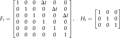
Here, we use linear process and measurement models. Moreover, we assume that the velocity between successive frames is constant. The frame rate of our cameras (30 fps) is sufficiently high to warrant this assumption. We define the state vector of each target based on its position and speed. More precisely, where x_it and v_it are position and velocity in each dimension. On the basis of these assumptions, F_t and H_t are as follows:

3.3

where Δt is the time step-size. The KF, as other Bayesian filters, has two steps: prediction and update. In the prediction step, the current state is predicted using the previous state and the process model. This estimated state is updated by including information from the current observation. Let be the estimated state vector of the target at time m after having observations up to and including time n. Then

3.4

We need to know the correspondence between measurements and targets to be able to perform the update step for each target. We use the Hungarian algorithm to find an optimized solution for this bipartite assignment problem.

We define a_t(i, j) to be the cost of each assignment between the predicted position of the ith target and the jth measurement at time t. The Hungarian algorithm finds the assignment with minimum . After finding assignments, states are updated and we get the state of the current time, which we use for prediction at the next time point, and so on. Figure 4 shows our approach for measurement correspondence and tracking.

Figure 4.

Tracking scheme: Hungarian algorithm is used for associating measurements to targets. (Online version in colour.)

4. Implementation and evaluation

In this section, we describe the hardware and software implementation of our approach.

4.1. Hardware

We constructed a tracking rig composed of four calibrated and synchronized PointGrey Grasshopper digital cameras mounted on the camera rig, each fitted with an Edmund optics 88 mm megapixel fixed focal lens (figure 5). The cameras are connected with FW800 PCI-E cards to a computer running two Intel 64-bit Quad Core Xeon Processors (2.8 GHz per core) with 8 GB of RAM. For some experiments, we added two more cameras to obtain high-resolution images (see §5.2.1).

Figure 5.

Camera system set-up.

4.2. Software

All building blocks of our tracking system (figure 1), including acquisition of images from cameras, silhouette detection and extraction of two-dimensional measurements, three-dimensional reconstruction and tracking algorithms, are implemented in Microsoft Visual C⁺⁺ 2005 using the Point Grey SDK and OpenCV libraries. Trackfix (§4.6) is implemented also in C⁺⁺ and uses the QT library (http://qt.nokia.com/) to provide an intuitive graphical user interface (GUI) for the user. Our trajectory analysis and automated behaviour recognition (§5) were implemented in Matlab using Statistics Toolbox v. 7.5.

4.3. Camera calibration

To calibrate the cameras, we chose to use freely available software called Camera Calibration Tool (http://www.cs.ucl.ac.uk/staff/Dan.Stoyanov/calib/). This software implements Zhang's [41] method for camera calibration. To calibrate each camera, we need to have images of a planar pattern (e.g. the checkerboard) in at least two different orientations. We used a 10 × 10 checkerboard in which each block was 5 × 5 mm. To have accurate calibration, we used five images of the checkerboard with different orientations for each camera.

4.4. Three-dimensional reconstruction evaluation

To evaluate the performance of seq-H in terms of accuracy of three-dimensional reconstructed points, we performed two sets of experiments. First, we put one fly in the container and recorded video with four calibrated cameras for 30 min. A typical two-dimensional image of the fly is approximately 10 × 20 pixels. We then used the proposed method to reconstruct the three-dimensional positions of the fly over time. Reconstructed three-dimensional points were projected back into each two-dimensional view. The back-projection error is defined as the Euclidean distance between the centroid of the fly in the original two-dimensional image, and its back-projection from the reconstructed position of the fly in three-dimensional space. Figure 6 shows the histogram of the back projection error in these views. The average back projection error is 1.75 pixels with a standard deviation of 1.8 pixels.

Figure 6.

Histogram of back projection error. (Online version in colour.)

To measure the efficiency of the Seq-H algorithm with different numbers of flies, in the next experiment we used synthetic data. Because there is no general consensus for a movement model of flies, we generated our ground truth trajectories by tracking a single real fly. We made a set-up with one fly inside a hemispherical dome (as shown in figure 3) and reconstructed the three-dimensional trajectory of a single fly inside the dome for around 108 000 frames (1 h of video). This three-dimensional trajectory was used to build a ground truth database. We randomly chose fragments of 150 frames from ground truth database and treated each of them as a ‘ground truth path’ for a single fly. The starting position of each fly was chosen randomly inside the dome and three-dimensional paths were shifted accordingly. After generating three-dimensional trajectories (150 frames each) for the desired number of flies, we projected them on multiple two-dimensional views to obtain two-dimensional measurements in camera views. To mimic the real-world scenario, we added Gaussian noise with mean zero and standard deviation of five pixels independently to both coordinates of all targets in all views. We used these noisy measurements as input to our algorithm.

We tested our algorithm by corresponding 10, 50 and 100 flies for 150 frames across multiple views. To measure the correspondence efficiency of Seq-H, we defined an intuitive and useful measure, the normalized reconstruction error (NRE). For a single time frame, we computed the minimum cost one-to-one matching between ground truth and reconstructed three-dimensional points. NRE is defined as the average Euclidean distance between matched ground truth and reconstructed three-dimensional points. We then normalize this parameter by dividing by the number of targets in each view. In every trial, we corresponded flies for each of 150 frames and averaged NRE values for them. We repeated this process and averaged the values obtained over five independent trials, with randomly chosen fragments from ground truth database. NRE values for 10, 50 and 100 targets were 0.06, 0.12 and 0.44 cm, respectively, which shows that the three-dimensional reconstructed points are accurate.

4.5. Tracking evaluation

We used two parameters, trajectory fragmentation factor (TFF) and number of bad frames (NBF), to evaluate the tracking accuracy. They are defined as follows:

TFF is a metric for measuring the accuracy of a tracker. We adopted this metric from [42]. TFF measures the number of acquired trajectories used to match one ground truth trajectory in a video segment. The ideal score of TFF is 1, which means the target has been perfectly tracked; the worst score is the number of flies in the experiment, which means the fly has been mixed up with all other flies during a tracking period. Figure 7 describes the TFF parameter in more detail. Figure 7a,b show the ground truth trajectories for two flies. Assume a mixing happens between fly 1 and fly 2. As shown in figure 7, to generate the ground truth trajectory (a) we need to use both the computed trajectories (c) and (d). In this case, the TFF is equal to 2.

Figure 7.

(a–d) Trajectory fragmentation factor (TFF) explanation. (a,b) Ground truth trajectories; (c,d) computed trajectories. (Online version in colour.)

NBF is the number of problematic frames in a video segment where any switching between identity of flies happens.

In general, both TFF and NBF values are dependent on the length of the video. Here, we chose the length of each video segment to be 1000 frames. To evaluate the tracking performance, we performed experiments with different numbers of flies, from one to seven, housed in a dome-shaped container with a radius of 50 mm (figure 3). For each trial, we recorded videos of 30 min duration at a resolution of 640 × 480 and a frame rate of 30 fps. We used four cameras and applied our software to process the videos and extract trajectories. We randomly chose 10 segments of video for each trial and manually checked them. Specifically, we counted all frames where there was a switching between flies (NBF). Moreover, we kept a record of the identity of flies that were mixing with each other and calculated TFF, based on these records. The reported results are the average of 10 segments for each trial.

As is shown in table 1, the average number of bad frames is low. For one and two flies, we do not have any bad frames and in the worst case, the average number of bad frames is 5.1 in 1000. Moreover, we can see from table 1 that as the number of flies increases, we have a higher TFF; this is expected because there is more chance of switching between flies in a larger group.

Table 1.

Performance of the tracking system in terms of TFF and NBF and average time for processing one frame.

no. of flies	avg. TFF	avg. NBF	time (ms)
1	1.00	0	21.00
2	1.00	0	21.00
3	1.53	1.3	21.30
4	1.72	2.2	22.07
5	1.68	2.1	22.90
6	2.13	5.1	22.75
7	1.48	4.7	23.00

4.5.1. Processing time analysis

We measured the running time of our approach by averaging the time taken for each step of processing over 15 000 frames (table 1). The most time-consuming step in our system is video acquisition and silhouette detection, which take up almost 95 per cent of the processing time for the single fly case (about 20 ms per frame). The video acquisition and silhouette detection are in practice independent of the number of flies. Silhouette detection is completely parallelized for each camera and the pixels in each frame. Despite the fact that our set-up consists of a single computer, the running time of our approach is comparable to Straw et al. [22]. As shown in table 1, we can process half an hour of seven-fly video recorded at 30 fps in about 21 min. This shows that the proposed approach could be used in real time.

4.6. Flagging and TrackFix

As discussed in §4.5, if we can fix bad frames, we obtain the three-dimensional trajectory of each individual fly without confusion with other flies. To find those frames in an automated fashion, we propose a flagging scheme that marks ‘risky’ frames while we are processing videos. An ideal flagging system marks all problematic frames while avoiding false positives. After some visual inspection, we have found the most important indicators to decide whether a frame is risky or not: losing measurements in more than two views, having no measurement for more than a few frames and wrong correspondence. Frames in which more than two flies are merged or are too close to each other are often those from which we do not get measurements from some flies. In these frames, there is a high probability of mixing between flies. On the basis of these observations, we flag frames that do not have enough measurements and/or the correspondence error (see §3.4) is large.

We used our flagging method in the experiments mentioned in §4.5. Accumulated results for all fragments for each experiment are reported in table 2. As can be seen from the table, our flagging method is quite efficient. The average number of FN is small, which shows that we rarely miss a risky frame. By adjusting the threshold for correspondence error and number of missing measurements, one can change specificity and sensitivity. In our experiments, around 10 per cent of frames were flagged. Once problematic frames are flagged, we fix them using a utility, called TrackFix, that we have developed for this purpose.

Table 2.

Flagging performance: true positive (TP), true negative (TN), false positive (FP), false negative (FN), sensitivity and specificity. Asterisk stands for undefinable.

no. of flies	TP	TN	FP	FN	specificity (%)	sensitivity (%)
2	0	994.7	1.3	0	100	*
3	1	893.2	26.9	0.3	96	87
4	2.2	816.9	35.0	0	95	100
5	1.8	883.6	24.4	0.3	97	83
6	4.7	822.9	42.0	0.2	95	95
7	4.7	669.5	31.9	0	95	100

TrackFix provides an intuitive GUI for someone to perform this task efficiently. Once a user starts watching flagged frames, if they see any switching between flies, they can select the ‘fix this frame’ option and correct the frame. All frames that occur after the corrected frame are automatically corrected based upon the mix-up in the previous frame, and hence consistency of trajectories is maintained in all operations of TrackFix. Another useful feature in TrackFix is the possibility of correcting two-dimensional measurements, which allows one to correct errors in silhouette detection (§3.2). This, in turn, leads to a low number of flags after reprocessing the video.

4.6.1. Merging and splitting

In experiments, there are some situations in which two individuals move or stay very close to each other for a considerable amount of time, for example when mating happens. In these cases, trajectories of flies are merged and they are not distinguishable from each other. Our approach is to track both individuals as one until they split. Merging and splitting frames are automatically recognizable from two-dimensional measurements and reconstructed three-dimensional trajectories. Thus, on top of our flagging scheme described in previous section, we make sure that splitting frames are also flagged so that a user can check those frames and fix the tracks if there is any mixing between identities.

5. Experimental applications

In this section, we present some experimental possibilities that our system provides for different types of experiments. Our first pilot experiment is activity level and movement analysis of two flies. We present two further experiments to demonstrate the capability of our approach for automating behaviour detection.

5.1. Activity level and movement analysis

We present a simple pilot experiment and preliminary analysis of trajectories to illustrate the usage of our approach. We put two flies in a Petri dish with a radius of 90 mm and height of 9 mm and recorded synchronized 30 fps videos, using four calibrated cameras, for 15 min (figure 8a). After running the tracking software, there was only one frame of 27 000 that needed to be fixed. We fixed this frame and acquired true three-dimensional trajectories of the two flies.

Figure 8.

(a) Container (dashed line, fly 1; solid line, fly 2). (b) activity level of two flies during the experiment (c) two-dimensional trajectory of fly 1 (d) two-dimensional trajectory of fly 2 (e) two-dimensional position histogram of fly 1 (f) two-dimensional position histogram of fly 2 (g) Speed colour-coded trajectory of fly 1 (h) Speed colour-coded trajectory of fly 2. (Online version in colour.)

Figure 8c–f shows the two-dimensional trajectories of these flies and the histogram of two-dimensional positions of the flies, respectively. As can be seen, fly 1 spends most of the time on the edge, while fly 2 stays more or less in the middle of the container. By calculating the speed of flies over the time, a measure of activity level is obtained. Figure 8b shows the activity level of flies over time. As can be seen, fly number 1 was active for the first 4 min, when fly 2 started to be active as well. After 10 min, the activity level of fly 2 decreased again. Figure 8g,h shows three-dimensional trajectories of the flies, colour coded by their speed. By looking at this figure and figure 8d,e we can infer that although fly 2 made some fast movements, he was mostly stationary at some location close to the middle of the container.

5.2. Automated behaviour analysis

We provide a framework based on machine-learning for automating annotation of different behaviours such as chasing, mating and aggression. This will save researchers from the laborious task of manually annotating videos and provides high-throughput data of individual and social behaviour of Drosophila.

We trained a support vector machine (SVM) with linear kernel function for behaviour classification. We used sequential minimal optimization for training [43]. The input features for the SVM are the distance between two flies, the speed of each fly and the angle between their trajectories. We created a training and a testing set for each experiment. The results reported in this section are based on our performance on test sets. Details of training and test sets are provided for each experiment.

5.2.1. Courtship experiments

Courtship is a complicated behaviour in Drosophila. One of the most common approaches for studying courtship is to put flies in small containers and record short videos (e.g. on the order of 10 min) and annotate videos manually. We show here that this task is highly automatable. To evaluate our approach, we ran 10 experiments pairing a single male and female and recording their interaction for 1 h. Flies were from a wild-type isofemale line from Montgomery, Alabama. Our recording settings and container were the same as §4.5. Videos were manually annotated for courtship events by an expert. More specifically, for each second in the video, the expert determined whether courtship had happened or not. We used the first experiment as the training set. The training sample size was 3600 (one sample per second). We trained the SVM for annotating the other nine experiments automatically. We compared the automated annotations with manual annotation given by the expert. As shown in table 3, we have high specificity and sensitivity for test experiments. We have a very small number of FNs; on average, we miss 27 s in a 1 h video. In table 3, copulation time is included in the accuracy assessment. If copulation time is excluded, there is a slight improvement in specificity (from 95.7% to 97.1%) and a small decrease in sensitivity (from 95.9% to 91.5%); detailed data are not shown. Figure 9 shows a graphical comparison between manual and automated annotation for trial 5. This demonstrates that our system is capable of finding courtship instances, and provides the opportunity to do experiments in a dome with diameter 10 cm instead of a small courtship chamber in which flies do not have much freedom to move.

Table 3.

Courtship detection performance: true positive (TP), true negative (TN), false positive (FP), false negative (FN), sensitivity and specificity.

trial no.	TP	TN	FP	FN	specificity (%)	sensitivity (%)
1	536	2877	18	168	76.1	99.4
2	1486	2061	23	29	98.1	98.9
3	2106	1352	120	21	99.0	91.8
4	1280	1998	312	9	99.3	86.5
5	2208	1354	4	33	98.5	99.7
6	1831	1587	130	51	97.3	92.4
7	1962	1575	25	37	98.1	98.4
8	2192	1331	34	42	98.1	97.5
9	1477	2030	67	25	98.3	96.8
average	1675.3	1796.1	81.4	46.1	95.9	95.7

Figure 9.

Comparison between (b) manual and (a) automated annotation for trial 5. (Online version in colour.)

5.2.2. Social behaviour analysis

Courtship experiments are usually carried out with one male and one female. However, courtship as well as some other social interactions are important to study when individuals are in a larger group. We performed a pilot experiment to show how our system can be used for analysing interaction between two individuals in a group. We evaluated our performance for detecting aggression (i.e. lunging, tussling and boxing) [44], chasing and mating in a group of three flies, two males (M1 and M2) and one female (F).

First, we put the two males in the container (figure 3), and after 1 h we introduced a female to the group. Flies were wild-type inbred lines from Raleigh, NC. The settings for recording videos were similar to the previous experiment, but we added two more cameras to record high-resolution images (1024 × 768) with lower frame rate (15 fps) synchronized with the other four cameras. These high-resolution images provided more details for the expert annotating the videos. Similar to the previous experiment, video was annotated by an expert and all of the two-way interactions between individuals (M1–M2, M1–F, M2–F) were indicated. We extracted three-dimensional trajectories in 1 h of video and fixed the flagged frames to avoid any error in trajectories. As training set, we randomly chose 65 per cent of the frames and used the rest of the frames as a test set to measure our performance. We kept the input features and the training method for the SVM the same as in the courtship experiments. We repeated the whole process of making training and test sets 10 times to mitigate the effects of bias. The results in table 4 give the average of these replicates.

Table 4.

Performance on social behaviours (asterisks stand for undefinable).

	individuals	chasing	mating	aggression
sensitivity (%)	F and M1	99.05	*	*
	M1 and M2	81.85	*	94.42
	F and M2	81.37	92.38	*
specificity (%)	F and M1	88.00	*	*
	M1 and M2	91.30	*	78.56
	F and M2	80.60	84.33	*

As is shown in table 4, sensitivity and specificity are high for all behaviours. Entities in the table for which there were no frames with that specific behaviour are marked with an asterisk. For example, there was no mating between M1 and F and no aggression between F and M2. Sensitivity and specificity for chasing and mating is high. However, there is still some room for improvement for detecting aggression. Training an SVM with more samples should improve the performance.

6. Conclusion

We have developed a tool that enables us to detect and keep track of multiple flies in a three-dimensional arena for a long period of time. Our system opens the door to many animal behaviour studies that were not previously feasible. There are several features that make this system unique. First, multiple individuals can interact in a three-dimensional space that has ethologically relevant features (such as food) and we can keep track of each individual's position, as well as their interactions, for a long period of time. Most of the current systems, such as [23,25], track individuals for short periods (on the order of seconds), while we use our system to track multiple flies for hours. This gives us the opportunity to investigate behaviours that need more time to occur. Moreover, it enables us to study changes in behaviour over time.

While in one study [35], movement analysis of one fly is reported, their approach is unable to measure activity of individuals in a group. There are other studies that have reported aggregated activity analysis for a group of flies [24,25]. However, the problem with this approach is that the difference between individuals is ignored. As we showed in §5.1, the activity levels of two individuals were quite different at different times. The simple approach of aggregating activity level disregards the differences between individuals and can lead to erroneous conclusions. Because we are able to provide three-dimensional trajectories of each individual precisely, we can provide accurate analysis of movement and activity level for each fly.

There are a few behavioural analysis assays, such as [20,21], which try to automate quantification of behavioural traits. However, the main disadvantage of their system is that it is in two-dimensional. Our system is the first of its kind that can provide high-throughput data for behavioural studies in a three-dimensional environment. In this paper, we presented results for interactions such as chasing, aggression and mating. Because we are using a machine-learning approach, instead of hard cut-offs or manual thresholds, our system is highly adaptable for different types of behaviour. Once the user provides training samples with manually annotated frames, an SVM can be trained for that specific behaviour and all other sample videos can be annotated automatically for that behaviour.

Our system is highly portable and can be easily reproduced. The physical set-up can fit in a 70 × 70 × 70 cm³ space and we use a low-end workstation for storing and analysing videos. Our system offers a complete package for recording, tracking, fixing tracks and behaviour analysis. Because it is readily adaptable for different types of experiments, we expect it to be used in many different behavioural studies.

References

- 1.Partridge BL, Pitcher T, Cullen M, Wilson J. 1980. Behavioral ecology and sociobiology. The three-dimensional structure of fish schools. Behav. Ecol. Sociobiol. 288, 277–288 10.1007/BF00292770 (doi:10.1007/BF00292770) [DOI] [Google Scholar]
- 2.Kane AS, Salierno JD, Gipson GT, Molteno TCA, Hunter C. 2004. A video-based movement analysis system to quantify behavioral stress responses of fish. Water Res. 38, 3993–4001 10.1016/j.watres.2004.06.028 (doi:10.1016/j.watres.2004.06.028) [DOI] [PubMed] [Google Scholar]
- 3.Zhou J, Clark CM. 2006. Autonomous fish tracking by ROV using monocular camera. In CRV06: Proc. Third Canadian Conf. on Computer and Robot Vision, Quebec City, Canada, June 2006, pp. 68–76 Washington, DC: IEEE [Google Scholar]
- 4.Wark AR, Greenwood AK, Taylor EM, Yoshida K, Peichel C. 2011. Heritable differences in schooling behavior among threespine stickleback populations revealed by a novel assay. PLoS ONE 6, e18151. 10.1371/journal.pone.0018316 (doi:10.1371/journal.pone.0018316) [DOI] [PMC free article] [PubMed] [Google Scholar]
- 5.Butail S, Paley D. 2012. Three-dimensional reconstruction of the fast-start swimming kinematics of densely schooling fish. J. R. Soc. Interface 9, 77–88 10.1098/rsif.2011.0113 (doi:10.1098/rsif.2011.0113) [DOI] [PMC free article] [PubMed] [Google Scholar]
- 6.Branson K, Belongie S. 2005. Tracking multiple mouse contours (without too many samples). IEEE Comp. Soc. Conf. on Computer Vision Pattern Recognition, San Diego, CA, 20–26 June 2005, pp. 1039–1046 Washington, DC: IEEE [Google Scholar]
- 7.Spink AJ, Tegelenbosch RA, Buma MO, Noldus LP. 2001. The EthoVision video tracking system: a tool for behavioral phenotyping of transgenic mice. Physiol. Behav. 73, 731–744 10.1016/S0031-9384(01)00530-3 (doi:10.1016/S0031-9384(01)00530-3) [DOI] [PubMed] [Google Scholar]
- 8.Pistori H, Odakura VVVA, Monteiro JBO, Gonçalves WN, Roel AR, de Andrade Silva J, Machado BB. 2010. Mice and larvae tracking using a particle filter with an auto-adjustable observation model. Pattern Recognit. Lett. 31, 337–346 10.1016/j.patrec.2009.05.015 (doi:10.1016/j.patrec.2009.05.015) [DOI] [Google Scholar]
- 9.Ballerini M., et al. 2008. Empirical investigation of Starling flocks: a benchmark study in collective animal behaviour. Anim. Behav. 76, 201–215 10.1016/j.anbehav.2008.02.004 (doi:10.1016/j.anbehav.2008.02.004) [DOI] [Google Scholar]
- 10.Cavagna A, Giardina L, Orlandi A, Parisi G, Procaccini A. 2008. The STARFLAG handbook on collective animal behaviour. II. Three-dimensional analysis. Anim. Behav. 76, 237–248 10.1016/j.anbehav.2008.02.003 (doi:10.1016/j.anbehav.2008.02.003) [DOI] [Google Scholar]
- 11.Betke M, Hirsh D, Bagchi A, Hristov N, Makris N, Kunz T. 2007. Tracking large variable numbers of objects in clutter. In IEEE Conf. on Computer Vision and Pattern Recognition, 2007 (CVPR07), Minneapolis, MN, 18–23 June 2007, pp. 1–8 Washington, DC: IEEE. [Google Scholar]
- 12.Theriault D, Wu Z, Hristov N, Swartz S. 2010. Reconstruction and analysis of 3D trajectories of Brazilian free-tailed bats in flight. In 20th Int. Conf. on Pattern Recognition, (figure 2), Istanbul, Turkey, August 2010, pp. 1–4. Washington, DC: IEEE. [Google Scholar]
- 13.Tian X. 2006. Direct measurements of the kinematics and dynamics of bat flight. Bioinspir. Biomimetics 1, S10–S18 10.1088/1748-3182/1/4/S02 (doi:10.1088/1748-3182/1/4/S02) [DOI] [PubMed] [Google Scholar]
- 14.Rayner J. 1985. Three-dimensional reconstruction of animal flight paths and the turning flight of microchiropteran bats. J. Exp. Biol. 265, 247–265 [Google Scholar]
- 15.Veeraraghavan A, Chellappa R, Srinivasan M. 2008. Shape-and-behavior encoded tracking of bee dances. IEEE Trans. Pattern Anal. Mach. Intell. 30, 463–476 10.1109/TPAMI.2007.70707 (doi:10.1109/TPAMI.2007.70707) [DOI] [PubMed] [Google Scholar]
- 16.Khan Z, Balch T, Dellaert F. 2005. MCMC-based particle filtering for tracking a variable number of interacting targets. IEEE Trans. Pattern Anal. Mach. Intell. 27, 1805–1819 10.1109/TPAMI.2005.223 (doi:10.1109/TPAMI.2005.223) [DOI] [PubMed] [Google Scholar]
- 17.Khan Z, Balch T, Dellaert F. 2006. MCMC data association and sparse factorization updating for real time multitarget tracking with merged and multiple measurements. IEEE Trans. Pattern Anal. Mach. Intell. 28, 1960–1972 10.1109/TPAMI.2006.247 (doi:10.1109/TPAMI.2006.247) [DOI] [PubMed] [Google Scholar]
- 18.Ramazani R, Krishnan H, Bergeson S, Atkinson N. 2007. Computer automated movement detection of the analysis of behavior. J. Neurosci. Methods 167, 171–179 10.1016/j.jneumeth.2007.01.005 (doi:10.1016/j.jneumeth.2007.01.005) [DOI] [PMC free article] [PubMed] [Google Scholar]
- 19.Grover D, Tower J, Tavaré S. 2008. O fly, where art thou? J. R. Soc. Interface 5, 1181–1191 10.1098/rsif.2007.1333 (doi:10.1098/rsif.2007.1333) [DOI] [PMC free article] [PubMed] [Google Scholar]
- 20.Branson K, Robie A, Bender J, Perona P, Dickinson MH. 2009. High-throughput ethomics in large groups of Drosophila. Nat. Methods 6, 451–457 10.1038/nmeth.1328 (doi:10.1038/nmeth.1328) [DOI] [PMC free article] [PubMed] [Google Scholar]
- 21.Dankert H, Wang L, Hoopfer ED, Anderson DJ, Perona P. 2009. Automated monitoring and analysis of social behavior in Drosophila. Nat. Methods 6, 297–303 10.1038/nmeth.1310 (doi:10.1038/nmeth.1310) [DOI] [PMC free article] [PubMed] [Google Scholar]
- 22.Straw AD, Branson K, Neumann T. R, Dickinson MH. 2010. Multi-camera real-time three-dimensional tracking of multiple flying animals. J. R. Soc. Interface 8, 395–409 10.1098/rsif.2010.0230 (doi:10.1098/rsif.2010.0230) [DOI] [PMC free article] [PubMed] [Google Scholar]
- 23.Wu H, Zhao Q, Zou D, Chen Y. 2011. Automated 3D trajectory measuring of large numbers of moving particles. Opt. Express 19, 7646–7663 10.1364/OE.19.007646 (doi:10.1364/OE.19.007646) [DOI] [PubMed] [Google Scholar]
- 24.Inan O, Marcu O, Sanchez M, Bhattacharya S, Kovacs G. 2011. A portable system for monitoring the behavioral activity of Drosophila. J. Neurosci. Methods 202, 45–52 10.1016/j.jneumeth.2011.08.039 (doi:10.1016/j.jneumeth.2011.08.039) [DOI] [PubMed] [Google Scholar]
- 25.Kohlhoff K, Jahn T, Lomas D, Dobson C, Crawther D, Vendruscolo M. 2011. The iFly system for automated locomotor and behavioural analysis of Drosophila melanogaster. Integr. Biol. 3, 755–760 10.1039/c0ib00149j (doi:10.1039/c0ib00149j) [DOI] [PMC free article] [PubMed] [Google Scholar]
- 26.Reiser M. 2009. The ethomics era? Nat. Methods 6, 413–414 10.1038/nmeth0609-413 (doi:10.1038/nmeth0609-413) [DOI] [PubMed] [Google Scholar]
- 27.Anonymous 2009. No fruit fly an island?. Nat. Methods 6, 395. 10.1038/nmeth0609-395 (doi:10.1038/nmeth0609-395) [DOI] [PubMed] [Google Scholar]
- 28.Zou D, Chen YQ. 2009. Acquiring 3D motion trajectories of large numbers of swarming animals. In IEEE Int. Conf. on Computer Vision (ICCV) Workshop on Video Oriented Object and Event Classification, Kyoto, Japan, September 2009, pp. 593–600 Washington, DC: IEEE. [Google Scholar]
- 29.Kuo Ch, Huang C, Nevatia R. 2010. Multi-target tracking by on-line learned discriminative appearance models. In IEEE Conf. on Computer Vision and Pattern Recognition (CVPR), San Francisco, CA, June 2010, pp. 685–692 Washington, DC: IEEE. [Google Scholar]
- 30.Zhou SK, Chellappa R, Moghaddam B. 2004. Visual tracking and recognition using appearance-adaptive models in particle filters. IEEE Trans. Image Process. 13, 1491–506 10.1109/TIP.2004.836152 (doi:10.1109/TIP.2004.836152) [DOI] [PubMed] [Google Scholar]
- 31.Hartley RI, Zisserman A. 2004. Multiple view geometry in computer vision, 2nd edn Cambridge, UK: Cambridge University Press [Google Scholar]
- 32.Wu Z, Hristov N, Hedrick T, Kunz T, Betke M. 2010. Tracking a large number of objects from multiple views. In IEEE Int. Conf. on Computer Vision (ICCV), Kyoto, Japan, September 2009, pp. 1546–1553 Washington, DC: IEEE. [Google Scholar]
- 33.Zou D, Zhao Q, Wu HS, Chen YQ. 2009. Reconstructing 3D motion trajectories of particle swarms by global correspondence selection. In IEEE Int. Conf. on Computer Vision (ICCV). Workshop on video oriented object and event classification, Kyoto, Japan, September 2009, pp. 1578–1585. Washington, DC: IEEE [Google Scholar]
- 34.Eshel R, Moses Y. 2008. Homography based multiple camera detection and tracking of people in a dense crowd. In 2008 IEEE Conf. on Computer Vision and Pattern Recognition (CVPR08), Anchorage, AK, June 2008, pp. 1–8 Washington, DC: IEEE. [Google Scholar]
- 35.Zou S, Liedo P, Altamirano-Robles L, Cruz-Enriquez J, Morice A, Ingram D, Kaub K, Papadopoulos N, Carey J. 2011. Recording lifetime behavior and movement in an invertebrate model. PLoS ONE 6, pe18151. 10.1371/journal.pone.0018151 (doi:10.1371/journal.pone.0018151) [DOI] [PMC free article] [PubMed] [Google Scholar]
- 36.Piccardi M. 2004. Background subtraction techniques: a review. In 2004 IEEE Int. Conf. Systems, Man and Cybernetics, The Hague, The Netherlands, 10–13 October 2004, pp. 3099–3104 Washington, DC: IEEE [Google Scholar]
- 37.Koller D, Weber J, Huang T, Malik J, Ogasawara G, Rao B, Russell S. 1994. Towards robust automatic traffic scene analysis in real-time. In Proc. of Int. Conf. on Pattern Recognition (ICPR), Jerusalem, Israel, October 1994, pp. 126–131 Washington, DC: IEEE [Google Scholar]
- 38.Blackman S. 2004. Multiple hypothesis tracking for multiple target tracking. IEEE A&E Syst. Mag. 19, 5–18 [Google Scholar]
- 39.Greenspan R, Freveur J. 2000. Courtship in Drosophila. Annu. Rev. Genet. 34, 205–232 10.1146/annurev.genet.34.1.205 (doi:10.1146/annurev.genet.34.1.205) [DOI] [PubMed] [Google Scholar]
- 40.Burkard R, Dell'Amico M, Martello S. 2009. Assignment problems, 1st edn. Philadelphia, PA: SIAM [Google Scholar]
- 41.Zhang Z. 2000. A flexible new technique for camera calibration. IEEE Trans. Pattern Anal. Mach. Intell. 22, 1330–1334 10.1109/34.888718 (doi:10.1109/34.888718) [DOI] [Google Scholar]
- 42.Perera AGA, Srinivas C, Hoogs A, Brooksby G, Hu W. 2006. Multi-object tracking through simultaneous long occlusions and split-merge conditions. In IEEE Conf. on Computer Vision and Pattern Recognition (CVPR06), New York, NY, 17–22 June 2006, pp. 666–673 Washington, DC: IEEE. [Google Scholar]
- 43.Platt J. 1998. Sequential minimal optimization: a fast algorithm for training support vector machines. Technical report: MSR-TR-98-14; Microsoft Research, Seattle, WA. [Google Scholar]
- 44.Nilsen S, Chan Y, Huber R, Kravitz E. 2004. Gender-selective patterns of aggressive behavior in Drosophila melanogaster. Proc. Natal Acad. Sci. USA 33, 12342–12347 10.1073/pnas.0404693101 (doi:10.1073/pnas.0404693101) [DOI] [PMC free article] [PubMed] [Google Scholar]