Robust, Globally Consistent, and Fully-automatic Multi-image Registration and Montage Synthesis for 3-D Multi-channel Images

Abstract

The need to map regions of brain tissue that are much wider than the field of view of the microscope arises frequently. One common approach is to collect a series of overlapping partial views, and align them to synthesize a montage covering the entire region of interest. We present a method that advances this approach in multiple ways. Our method (1) produces a globally consistent joint registration of an unorganized collection of 3-D multi-channel images with or without stage micrometer data; (2) produces accurate registrations withstanding changes in scale, rotation, translation and shear by using a 3-D affine transformation model; (3) achieves complete automation, and does not require any parameter settings; (4) handles low and variable overlaps (5 – 15%) between adjacent images, minimizing the number of images required to cover a tissue region; (5) has the self-diagnostic ability to recognize registration failures instead of delivering incorrect results; (6) can handle a broad range of biological images by exploiting generic alignment cues from multiple fluorescence channels without requiring segmentation; and (7) is computationally efficient enough to run on desktop computers regardless of the number of images. The algorithm was tested with several tissue samples of at least 50 image tiles, involving over 5,000 image pairs. It correctly registered all image pairs with an overlap greater than 7%, correctly recognized all failures, and successfully joint-registered all images for all tissue samples studied. This algorithm is disseminated freely to the community as included with the FARSIGHT toolkit for microscopy (www.farsight-toolkit.org).

I. Introduction

Many applications require high-resolution three-dimensional (3-D) imaging of regions that are much wider than the lateral field of view of the microscope. This is accomplished by collecting a series of partial views of the overall region of interest, and then combining them to form a synthetic image (montage or mosaic) covering the entire region (Capek et al., 2009, Becker et al., 1996, Al-Kofahi et al., 2002, Price et al., 2006). Achieving a seamless montage requires accurate registration (alignment) of the tiles along the lateral and axial dimensions. This is difficult when imaging wide regions of mammalian brain tissue (ranging from multiple millimeters to whole brains) at sub-cellular resolution. Solutions to this problem are essential for investigating diverse questions in neuroscience ranging from the study of cellular networks underlying learning and memory (Guzowski et al., 2005), to the reconstruction of cells with processes that extend over significant distances (Oberlaender et al., 2007), and characterization of brain tissue injury caused by the insertion of experimental neuroprosthetic devices (Bjornsson et al., 2008). In this type of work, thick brain tissue slices (10 – 1000μm) are imaged using 3-D fluorescence microscopes (confocal, multi-photon, etc.) using one or more channels (fluorophores). One peculiarity of such imaging methods is the anisotropy of the images with the axial dimension less well resolved compared to the lateral dimension, and the presence of spatial distortions and aberrations. Another peculiarity, rooted in physical causes, is the depth-dependent attenuation of the fluorescence signal. Additionally, there is mechanical imprecision in microscope stages along the lateral and axial dimensions as they execute a wide-ranging scanning pattern across the specimen to collect the image tiles. This is particularly problematic when scanning larger numbers of tiles, since small stage errors can accumulate and be compounded by mechanical hysteresis. Finally, one must often process legacy datasets that are collected without motorized stage micrometer data, or collected with stages that lack accurate motorized micrometers. Adjacent tiles may also be collected at different magnification in such cases where greater detail must be acquired only at specific locations within a larger region of interest. There is a need for computational methods that achieve accurate alignment and montaging of 3-D image tiles, while coping with the peculiarities and artifacts noted above.

The goal of this work is to advance the accuracy, robustness, scalability, and level of automation of 3-D montage synthesis in multiple ways.

• Our approach is designed to align an unorganized but laterally & axially overlapping collection of 3-D image tiles. It can cope with a lack of stage micrometer information. It uses a 3-D affine transformation that can cope with common image distortions.

• The method is designed to align adjacent tiles with low and variable overlap (lateral and axial offsets). Approximately 5-15% overlaps are usually adequate.

• By avoiding the accumulation of registration errors, it is scalable, allowing large montages to be constructed to achieve higher spatial extent and resolution. This is achieved by aligning all the images jointly, rather than sequentially yielding a globally consistent set of alignments. This is accomplished at an affordable computational cost.

• The method has a self-diagnostic ability, and can automatically identify pairs of images that have not been registered correctly, instead of delivering an incorrect result to the user.

• The algorithm is applicable to a broad range of biological images by exploiting alignment cues from any and all fluorescence channels (assuming that they are corrected for chromatic aberration by the microscope software/hardware) without the need for segmentation of specific biological entities.

• The algorithm is free of adjustable parameter settings. This issue has a direct impact on the practical usability of algorithms. This differentiates our work from many existing algorithms in the literature that require the user to provide initial estimates of registration parameters, and various other hints and settings in order to achieve satisfactory results (Appleton et al., 2005, Chow et al., 2006, Sun et al., 2006, Thevenaz & Unser, 2007).

Our goal is to make this robust and state-of-the-art computational method usable in a practical sense, and freely available to the microscopy community to enable unfettered adoption. To this end we have made efforts to minimize the computational requirements, and implemented the software in ways that enable it to be used on diverse types of computers. The algorithms described here are disseminated freely as part of the NIH funded Fluorescence Association Rules for Multi-Dimensional Insight (FARSIGHT; refer to Table 1 for a list of abbreviations used in this paper) toolkit for microscopy (www.farsight-toolkit.org).

Table I.

This table lists the abbreviations for jargon used within the text.

Acronym	Definition
FARSIGHT	Fluorescence Association Rules for Multi-Dimensional Insight
GDB-ICP	Generalized Dual-Bootstrap Iterative-Closest-Point
SIFT	Scale Invariant Feature Transform
NC	Normalized Cross-Correlation
MUSE	Minimum Unbiased Scale Estimator

II. Review of Current Methods

Manual and approximate methods for montage synthesis continue to be used widely. One such method is to project the 3-D images that are to be registered axially down to a pair of two-dimensional (2-D) images, and estimate the lateral stage shift from these images. Estimating the shift can be performed visually, or automatically (Beck et al., 2000). The outcome is good for flat viewing, but not adequate for volumetric visualization or 3-D image analysis (Bjornsson et al., 2008), since the two image stacks are not guaranteed to align along the axial dimension due to issues such as non-uniform specimen thickness. This problem is illustrated in Figure 1. To support studies that require 3-D analysis, accurate alignment of 3-D image stacks must be carried out laterally and axially.

Figure 1.

Illustrating the importance of fully three-dimensional (3-D) registration. Adjacent image stacks with an equal number of optical slices may still be offset axially relative to the objects in the tissue. (A) Two adjacent confocal stacks represented by horizontal rectangles, and hypothetical objects within the confocal image stacks represented by colored ovals. Arbitrarily registering the stacks using the top or bottom optical slice of the image stack does not yield an accurate montage. (B) One stack must be shifted along the z axis relative to the other. In practice, confocal image stacks often contain varying numbers of optical slices. Panels (C) and (D) are slice 30 from adjacent confocal stacks of rat brain tissue stained with a fluorescent antibody against the microglial-specific protein Iba-1. However, they are not the matching slices. For correct alignment, the stack in (D) should be shifted about 5 slices in the z-direction. Panel (E) shows slice 30 of the correctly aligned montage produced by our 3-D registration algorithm. Panels (C), (D), and (E) are taken from data set #2.

Much of the literature on image registration focuses on registering a pair of overlapping images- the so-called “pair-wise” registration. Several literature surveys are available (Lester & Arridge,1998, Hill et al., 2001, Maintz & Viergever, 1998, Makela et al., 2002, Gholipour et al., 2007, Brown, 1992, Zitova & Flusser, 2003). Two broad classes of algorithms have been described – intensity-based and feature-based. Intensity-based approaches optimize an objective function based on the correlation of image intensities (Capek & Krekule 1999, Appleton et al., 2005, Thevenaz & Unser, 2007) or measures such as mutual information (Capek & Krekule, 1999, Karen et al., 2003) between the pair of images being registered. The advantage of intensity-based methods is that they do not require the extraction of image landmarks or segmentation, so they are broadly applicable to images in any context. However, they are susceptible to imaging artifacts, such as non-uniform illumination, and are computationally expensive since the computer must operate upon the entire image volumes. On the other hand, feature-based techniques are driven by alignment of automatically detected “features” or landmarks, that can be the result of application-specific segmentation (Al-Kofahi et al., 2002, Becker et al., 1996) or simply generic features, such as closed contours (Bajcsy et al., 2006) and keypoints (Hsu et al., 2008, Sun et al., 2006). Unlike intensity-based methods, they are more tolerant of image artifacts and are computationally efficient since only small sub-regions of the image volumes (around the features) must be processed. However, the downside of feature-based algorithms is their dependence on the robustness and accuracy of feature extraction. To combine the advantages of intensity and feature-based approaches, some recent techniques limit the intensity-based alignment to small windows around salient points (Chow et al., 2006, Emmenlauer et al., 2009).

Many biomedical image registration algorithms require initial estimates to be provided by the user (Viola et al., 1997, Maes et al., 1997, Hsu & Loew, 2001). They also assume that there are no major changes in viewpoint between images. While this assumption is reasonable for PET/MR imaging, it does not hold for microscope images intended for montage synthesis, since it is desired to maximize the coverage with the fewest images. As a result, our images have major displacements and small overlaps, at least in the lateral (x – y) plane. For this reason, many algorithms designed specifically for microscopy data rely on positions of the scanning stage or manual pre-alignment (Thevenaz & Unser, 2007, Sun et al., 2006, Chow et al., 2006, Appleton et al., 2005, Karen et al., 2003). Automatic initialization can be achieved in a variety of ways including multi-resolution (Feldmar et al., 1997), image-wide measurements (Higuchi et al., 1995, Johnson & Hebert, 1998), phase-correlation (Slamani et al., 2006, Emmenlauer et al., 2009, Preibisch et al., 2009), invariant-indexing and initial matching of key points (Al-Kofahi et al., 2002), Hough transforms (Becker et al., 1996), minimal-subset random-sampling on the pre-matched correspondences (Chow et al., 2006, Fischler & Bolles, 1981), and multiple starting points (Jenkinson & Smith, 2001).

Common approaches for generating microscope montages involving more than 2 images include incrementally registering the partial montage with a new image that is not yet part of the montage (Becker et al., 1996, Karen et al., 2003, Chow et al., 2006), building the minimum/maximum spanning trees where the images are the nodes and the edges are valid transformations with weight assignment (Thevenaz & Unser, 2007), and finding the least-squares solution using the parameters or correspondences from a pair-wise registration (Hsu et al., 2008, Emmenlauer et al., 2009, Sun et al., 2006, Preibisch et al., 2009). The first approach suffers from heavy memory consumption since the size of the partial montage scales with the number of images involved, whereas the second approach lacks global consistency if more than two images share a common area. This results in an accumulation of small pair-wise alignment errors as one attempts to process an extended array of image tiles. Left unchecked, this makes it impossible to produce seamless/accurate/consistent montages of regions beyond a certain number of tiles (depending upon the extent of the drift errors).

III. Methodology

Given an unorganized and unordered collection of images, our method for achieving globally consistent multi-channel 3-D montaging operates in two steps, both of which are fully automatic. The first step performs 3-D pair-wise registration of all possible image pairs when no stage information is available (fewer registrations can be done when such data are available). This has the effect of registering most, if not all image pairs that overlap. The second step leverages the results of the pair-wise registrations to perform a joint registration of all the image tiles with global consistency. The outcome of the latter is a set of accurate spatial transformations between every pair of stacks that can be used to construct a 3-dimensional montage at the final stage. The individual steps are described in greater detail below.

Step 1: Robust Pair-wise Image Registration

Given a pair of image tiles denoted $I_r^{3D}$ and $I_m^{3D}$, respectively, the purpose of this step is to establish a preliminary estimate of the 3-D affine transformation that maps points in one image to the image space defined by the second image (Figure 2). Our method combines feature- and intensity-based registration approaches using all available image channels. The low overlap between the images implies the need for a robust registration algorithm that can handle outliers among matches. It is well known that a rigid transformation fails to account for small spatial distortions that exist between image pairs. Al-Kofahi et al. (2002), showed that an affine transformation models translation, rotation, scaling and shearing between two images is sufficiently accurate, yet of a manageably low dimension for registering 3-D microscopy images (Al-Kofahi et al., 2002). It accommodates a modest but realistic degree of deformation (usually arising from spatial aberrations) between adjacent images without incurring the massive computational cost of a fully deformable model. Even then, direct registration of a pair of 3-D images (especially if they are large) to fit an affine model can be computationally expensive since it contains 12 free parameters (dimensions). With this in mind, we make reasonable but non-limiting tradeoffs. Assuming that the user is acquiring a series of image tiles by shifting the stage, the spatial transformation from one image tile to the next is largely accounted for by the lateral shift – the contributions of rotation and shear in the 3-D space are much less in comparison. With this in mind, we decompose the problem into three substeps to reduce computation. First, we estimate the lateral shift between the images by registering the maximum-intensity axial projections at a low computational cost. Second, we estimate the shift along the axial dimension separately. The estimates from the first and second substeps are combined to generate an initial estimate of the full 3-D transformation. This estimate is refined using the intensity information from the estimated overlapping volumes to yield the pair-wise registration, as described further below.

Figure 2.

Illustrating preliminary estimation of the lateral offset for a pair of 5-channel images of the cortical surface (blue: nuclei, purple: Nissl, Green: microvasculature, yellow: microglia, red: astrocytes). Panels (A) and (B) show the maximum-intensity projections of the two adjacent optical stacks with all 5 channels overlaid. Panels (C) and (D) show the generic landmarks for these images overlaid on the fusion image derived by combining the 5-channel data into one. The yellow circles indicate corners and the yellow lines indicate the locations and normal directions of edge points. Panel (E) shows the alignment produced by the GDB-ICP pair-wise registration of the projection. The transformation computed from panels (C) and (D) was applied to the 5-color projections, and used to construct a 2-D montage of these two projection images. Images in this figure are taken from data set #2.

1. Initial estimation of lateral shift

This is performed on 2-D axial maximum-intensity projections, denoted $I_r^{2D}$ and $I_m^{2D}$ of the 3-D images $I_r^{3D}$ and $I_m^{3D}$, computed across all the channels. The computation across channels allows us to take advantage of alignment cues from any and all channels, while keeping the memory requirements modest compared to the direct alternative of processing multiple channels and then combining the cues. Figure 2(A & B) show two adjacent images of brain tissue containing 5 channels. Panels C & D show the composite projections overlaid with extracted landmarks. The yellow circles indicate corners and the yellow lines indicate the locations and normal directions of edge points. We perform 2-D alignment of the projected images using the Generalized Dual-Bootstrap Iterative-Closest-Point (GDB-ICP) algorithm (Yang et al., 2007), which is known for its robustness to low overlap, substantial orientation and scale differences, and large illumination (or photobleaching caused) image changes. Indeed, GDB-ICP aligns generic features, such as corners and edges, instead of segmented biologically meaningful entities such as cells. This avoids a dependence on image segmentation algorithms that are only available for some types of entities, and subject to errors of their own. Specifically, a set of multi-scale key points is extracted from each image (Lowe, 2004). A key point in $I_r^{2D}$ is matched against key points in $I_m^{2D}$ based on the similarity of the Scale Invariant Feature Transform (SIFT) descriptor (Lowe, 2004). Since each key point is associated with the location of the keypoint center, the major orientation of the gradient directions, and the scale in which the key point is extracted, it defines a local coordinate system that is sufficient to constrain a similarity transformation (scale, rotation, and translation) with its matching key point. A set of rank-ordered similarity transformations are generated from key point matches, and tested individually in succession. Because of the effectiveness of key point matching, it is seldom necessary to test more than 5 matches if correct matches exist between the two images. For each key point match, the initial pair-wise transformation is refined using the Dual-Bootstrap Iterative-Closest Point algorithm DB-ICP (Stewart et al., 2003), driven by matching of the generic features — corners and edges extracted in Gaussian-smoothed scale-space. The features are adaptively pruned to ensure an even distribution across the image. The refinement process starts from an initial local region defined by the key point match. The region is expanded to cover the entire overlap between images while refining the estimate and choosing the best transformation model as the region grows at a rate controlled by the uncertainty in the transformation estimate. To determine the correctness of the final transformation, measurements of alignment accuracy, stability in the estimate, and consistency in the matches are examined. The algorithm terminates as soon as one initial transformation is refined to the desired accuracy, or terminates with failure after exhausting all potential key point matches and returns no transformation. The result of a successful registration is a 2D affine transformation in the x-y plane, which captures the major displacement between the two volumes. Figure 2E shows the alignment generated by GDB-ICP.

2. Initial estimation of axial shift

The 2-D affine transformation resulting from the above step is denoted ${\theta }_{2D}^{\mathit{initial}}=\left[\begin{array}{cc}{A}_{2D}& t_{2D}\end{array}\right]$, where A_2D is an 2 × 2 affine parameter matrix and t_2D is the 2-D lateral translation. Using this transformation, we compute a pair of 3-D boxes, one for each image, that together define the region of overlap between the two images. For each image volume, the 3-D box is the smallest rectangle that encloses all the points within the overlapping area formed by the 2-D projected images. To estimate the shift in the axial direction (z), we compute the 0^th moments (center of mass) for each bounding box. Let c_r = (x_r, y_r, z_r) be the center of mass for $I_r^{3D}$ in the bounding box, and c_m=(x_m,y_m,z_m) for $I_m^{3D}$. Combining this with the initial guess of the lateral shift, the initial estimate of the 3-D affine transformation is given by:

$${\theta }_{3D}^{\mathit{initial}}=\left[\begin{array}{ccc}{A}_{2D}& 0& t_{2D}\\ 0& 1& z_r-z_m\end{array}\right].$$

3. Refinement of the initial 3-D transformation

This initial transformation ${\theta }_{3D}^{\mathit{initial}}$ is refined using a 3-D intensity-based registration algorithm that operates on the sub-volumes defined by the bounding boxes. This algorithm is implemented as part of the open source Insight Toolkit (Ibanez et al., 2003). It performs a regular-step gradient descent minimization of the inverse pixel-wise normalized cross-correlation (NC) error between volumes $I_r^{3D}$ and $I_m^{3D}$ defined below:

$$\mathit{NC}\left(r,m\right)=1-\frac{{\sum }_{i=1}^N\left(r_i\times m_i\right)}{\sqrt{{\sum }_{i=1}^N{r}_i^2\times }\sqrt{{\sum }_{i=1}^N{m}_i^2}},$$ (1)

where (r_i,m_i) is a corresponding pair of voxels from $I_r^{3D}$ and $I_m^{3D}$, respectively. This metric is in the range of [0,1] and is minimum when the images are in perfect alignment. This metric is insensitive to multiplicative intensity factors between the two images. Therefore, it is robust to linear illumination changes and is adequate for a well-run microscope. Another advantage of NC is its normalization, so a larger overlap does not result in a higher value. The final pair-wise transformation from image $I_m^{3D}$ to image $I_r^{3D}$ resulting from this refinement algorithm is written as follows:

$${\theta }_{m,r}^{3D}=\left[\begin{array}{cc}{A}_{3D}& T_{3D}\end{array}\right]=\left[\begin{array}{cccc}{a}_{00}& a_{01}& a_{02}& t_x\\ a_{10}& a_{11}& a_{12}& t_y\\ a_{20}& a_{21}& a_{22}& t_z\end{array}\right],$$

where the submatrix A_3D is a 3 × 3 affine transformation matrix, and the parameters T_3D = (t_x, t_y, t_z) are the refined estimates of the 3-D translation between the image pair.

Step 2: Joint Registration of Multiple Image Tiles

The pair-wise transformation estimates from the previous step ${\theta }_{m,r}^{3D}$ are not guaranteed to be globally consistent. The joint registration procedure performs a second round of refinements to achieve a globally consistent set of transformations. To illustrate the importance of this issue, consider the 4-image montage in Figure 3A. The blue box highlights one tile that we chose to treat as the “anchor” image, meaning that all other images are mapped to the coordinate frame represented by this image. This montage was constructed by pair-wise registration of 3 other images to the anchor image. The regions highlighted by the red ellipses highlight the inconsistency that arises from this procedure. The blurred details in these regions show alignment errors. Such errors have a magnified impact as one attempts larger montages, since even modest pair-wise registration errors can add up into a large-scale drift across the montage that can distort the geometry of the region being imaged. Furthermore, it is possible for some pair-wise registration operations to fail, although individual images are registered successfully with other images. This problem is best described in the language of graph (network) theory. If each image in the montage is represented as a node in a network, and each successful pair-wise registration is represented as a link, then the set of all successful pair-wise image registrations produces a graph that is not fully connected. In this language, pair-wise registrations on overlapping image pairs results in a connected graph that is turned into a fully connected graph by the joint registration procedure so that a transformation exists between every two images in the graph. After joint registration, any image can be chosen as the anchor image for montage synthesis.

Figure 3.

Illustrating the need for joint registration with global consistency. (A) A 4-image montage based on pair-wise registration. The blue box indicates the reference image for the montage. Corresponding points between the neighboring images are mapped inconsistently to different locations, resulting in blurry overlap regions outside the reference image, circled in red. (B) A montage of the same 4 images constructed with globally consistent joint registration where points are well aligned even outside the reference image space. The boxes outline the 4 images that were jointly registered. Images in this figure are from data set #2.

Several algorithms have been proposed for joint registration. Common approaches are to cascade the parameters of successful pair-wise transformations from any chosen image to the reference image, since the affine transformation model is closed under composition (Choe & Cohen, 2005, Gracias & Santos-Victor, 1999), and to build spanning trees for certain cost functions (Chow et al., 2006, Beck et al 2000, Thevenaz & Unser, 2007). These approaches are simple but lack global consistency—the corresponding points from a pair of non-reference images can map to different locations in the montage if they are outside the reference image, since only correspondences in the reference image space are constrained. Can and colleagues (2002) described an algorithm with global consistency for registration of 2-D retinal images. In this work, we extended this method to handle 3-D confocal images.

The joint registration algorithm treats each image in turn as the “anchor image,” which defines the coordinate reference space, and estimates the set of transformations that map all other images to this reference space. Without loss of generality, let the 3-D anchor image be denoted I₀, and the other images denoted {I_i}_i=1⋯N. For every image pair (I_m, I_n) with a pair-wise transformation, a set of point-wise correspondences denoted $C\left(m,n\right)=\left\{\left(p_i,{\theta }_{m,n}^{3D}\left(p_i\right)\right)\right\}$ is hypothesized, where {p_i } is a set of sampled points from image I_m. The joint registration problem is formulated as the minimization of a squared error between hypothesized and actual point correspondences, as quantified by the following objective function:

$$E\left({\theta }_{1,0},\cdots ,{\theta }_{N,0}\right)=\sum _{\left\{m,0\right\}\in P_D\left(p_{i,}{p}_j\right)\in C\left(m,0\right)}{\sum \Vert {\theta }_{m,0}\left(p_i\right)-p_j\Vert }^2+{\sum _{\left\{m,n\right\}\in P_I\left(p_{i,}{p}_j\right)\in C\left(m,n\right)}\sum \Vert {\theta }_{m,0}\left(p_i\right)-{\theta }_{n,0}\left(p_j\right)\Vert }^2,$$

where P_D contains image pairs that registered successfully with the anchor, and P_I contains the remaining successfully registered pairs. The first term of this objective function constrains the transformations mapping directly to the anchor, whereas the second term ensures global consistency for mapping images that do not overlap with the anchor image. Minimizing the above objective function is a linear problem amenable to efficient computation. We simply set the derivative of E(θ_1,0,⋯,θ_N,0 ) with respect to the transformation parameters to zero, and solve for the optimal parameters. Importantly, since no montage image is explicitly generated during processing, this operation can be performed on datasets containing any number of images using a standard laboratory computer equipped with sufficient memory for registering 2 images. Figure 3B shows greatly improved results produced by joint registration with global consistency for the same dataset as shown in Figure 3A.

Self-diagnosis

In the rare instances when keypoint features are too sparse for the GDB-ICP registration, the pair-wise algorithm can produce an incorrect transformation. It is impractical to validate every pair-wise transformation visually. To automate this process, the joint registration accepts pair-wise transformations with the NC value (eq 1) below a threshold value T that is determined adaptively for every image set using a robust error scale estimator. For this, we adopt the Minimum Unbiased Scale Estimator (MUSE) that automatically adjusts its estimate of error scale by determining the approximate fraction, which can be less than 50%, of pairs with an acceptable error (Miller & Stewart, 1996). The errors are assumed to be positive with a zero-mean normal distribution. The input to MUSE is the set of errors {NC(I_m,I_n)} for image pairs {(I_m,I_n)}. The threshold T is set to nσ, where σ is the scale estimated by MUSE and n = 4 for all our experiments. All pairs with NC(I_m,I_n) < T are included in the joint registration. It is crucial that pair-wise registration has this self-diagnostic capability, i.e. being able to reject almost all incorrect transformations, so that the errors of correctly registered pairs form a clear cluster far apart from the errors of mis-registered pairs. This leads to correct error scale estimation to include only the correct transformations, and all of them, in the joint registration.

Applications of the jointly estimated transformations

Once computed, the set of spatial transformations can be used to relate any two images in the set spatially regardless of their distance within the specimen. This is an enabling capability. For a start, it can be used to compute long-range distance measurements. Another application is 3-D montage synthesis. For this, any one image can be chosen as the anchor and all other images are transformed to the image space of the anchor image. For each non-anchor image, the coordinates of the 8 corner points are transformed to the anchor space so that the final size of the montage can be determined. To generate the image of the montage, the intensity value of each pixel in the montage is computed as the average intensity value of images that overlap at the given pixel. The memory consumption for montage synthesis scales with the size of the final montage – rapidly falling costs of computer memory make this very practical. The spatial transformations generated by our method can also be reused to compute “object mosaics”, i.e., mosaics of automated image segmentations conducted over each image tile. Second, it is possible to compute cytovascular maps of tissue on a much larger scale than was possible earlier (Bjornsson et al., 2008). Finally, it is possible to merge quantitative measurements from each tile. This can be used to perform large-scale data mining operations to identify patterns in brain tissue that occur over significant distances compared to the size of a single cell.

IV. Workflow Using Registration and Montage Synthesis Programs

The executable files used for pairwise registration, joint registration, and montage synthesis and the workflow for their use is depicted in Figure 4. For detailed instructions on the use of each file, including all optional switches for each executable, see the instructions included in the supplementary material and available online at http://www.farsight-toolkit.org/wiki/Registration_page. A brief explanation of the workflow required to go from acquired images to a final synthesized montage follows.

Figure 4.

Flowchart demonstrating the basic steps, including the inputs and outputs, for performing (in turn) pairwise registration, joint registration, and montage synthesis. Pairwise registration is performed multiple times (for each possible image pair) but is only depicted in the flowchart once; practically the user will perform this step as many times as required for the dataset before moving on to joint registration.

Given a set of images, the first step is to perform registrations of each pair of images using register_pair.exe. This executable takes two images for input, a “from” image and a “to” image; it does not matter which image in a pair is designated as “to” or “from”. This executable produces an XML file which contains the pairwise transformation data for the pair of images. The name of this file follows the syntax “<fromfilename>_to_<tofilename>_transform.xml” where <fromfilename> and <tofilename> are the names of the “from” image and “to” image, respectively, that the user designates.

Once all pairwise transformations are generated, the user then must generate the joint transformation using register_joint.exe. The input for this program is a plain text file that lists, one per line, the names of all the pairwise transformation XML files generated by register_pair.exe. The output is a file named joint_transforms.xml which contains the joint registration data for all the image pairs, and at this point the user is finished with registration of image data and can use this to generate a montage.

The principal program for synthesizing the final montage is mosaic_images.exe. This program takes the output joint transformation XML file from register_joint.exe, and the filename for an anchor image, as inputs. The anchor image is any of the original images in the set choice of image by the user is arbitrary and does not affect the results of the algorithm. There are several outputs from this program: an XML file containing information necessary for constructing the montage, such as the name of the anchor image and the transformations involved; a 2-dimensional flattened projection of the montage; and a directory containing tif files corresponding to the slices of the 3D montage. Due to the potentially large size of the synthesized 3-dimensional montage, the default behavior of this program is not to generate that file; however by setting a switch (see instructions in the supplementary file), a 3-dimensional tif file for the entire montage may be generated. Mosaic_images.exe is designed to output only grayscale images. For multi-channel images, as often are generated using confocal microscopy, the user may choose to generate a montage including all channels fused or a montage of a specific channel if selected. To generate a color montage to better differentiate information in different channels, for example, the image in Figure 5, the user may use available software, such as ImageJ (http://rsbweb.nih.gov/ij/), or our utility programs multi_channels_2D.exe and multi_channels_3D.exe. Both the utility programs take a file that lists, one per line, the montage files for single channels and their RGB components (see instructions in the supplementary file) and the name for the output file.

Figure 5.

Maximum intensity projection of the montage of Dataset #1 taken from the rat entorhinal cortex. The montage is 4,756×2,943×58 voxels in size. The blue channel shows the cell nuclei, and the green channel indicates the neurons. Spatial co-localization of green and blue signal (turquoise) indicates the locations of neurons. The confocal images were obtained from sections of rat brain sectioned horizontally and stained with the flurorescent nuclear dye To-Pro-3 iodide (Invitrogen) and the fluorescent secondary antibody Alexa Fluor 488 (Invitrogen) following initial labeling with a primary antibody against NeuN, which is expressed specifically in neurons.).

In order for register_pair.exe to function, it must be able to call the Generalized Dual-Bootstrap Iterative-Closest Point program. This can be accomplished either by placing the file gdbicp.exe in the same folder as the other programs for montage synthesis, or by designating the path to the file using a switch during execution of register_pair.exe (see the instructions in the supplementary material). Default image output is in tif format; viewing 3-dimensional tif files however requires a special image viewer such as Irfanview (http://www.irfanview.com/) or ImageJ (http://rsbweb.nih.gov/ij/)- opening a 3-dimensional tif in other image viewers (such as Photoshop) may only open the top image plane, or fail altogether.

For large numbers of image pairs, it quickly becomes tedious to manually run register_pair.exe for all possible image pairs; even when the correct image pairings are known a priori, it can be tedious to run this program sequentially. Since these programs are run from a command prompt, the user is highly encouraged to write a script that will batch process the entire image set. For convenience a Python script is included on the download page at http://www.farsight-toolkit.org/wiki/Registration_page for those users that do not have programming experience; this script requires an installation of Python to be usable. Finally, the images comprising Dataset #1 (below), and the final synthesized montage, are included for download from http://farsight-toolkit.org/data/Montage_synthesis/ and http://farsight-toolkit.org/data/Original_images_files/. Readers may use these files to verify that their downloads of our executable files are functioning correctly. The images and final synthesized montage for Datasets #2 and #3 are also available upon request from the authors.

V. Experimental Results

All the experiments were run fully automatically without any manual intervention or parameter optimization. As a visual confirmation, we generated and inspected 3-D montages (Figures 5 - 7) for 3 large data sets containing at least 50 images from various parts of the brain, and they were essentially seamless. Table II provides summary information for these 3 sample datasets collected in two different laboratories.

Figure 7.

This figure illustrates robustness of montage synthesis in coping with spatial distortion in the data set. Panel A shows three optical slices (16, 17, and 18) from the confocal stack collected at location H,05 as marked in panel B. Slice thickness is 0.7 microns. The immersion oil during collection of this data set was inadvertently contaminated with water, presumably altering the index of refraction of the immersion medium and resulting in spatial distortion between optical slices. Moving up and down through the collected image stack results in a “rippling” effect; the x-y positions of neuronal nuclei appear to jitter back and forth as one moves through adjacent slices in the z-plane. One can note the right-left shifts in position of two neuronal nuclei (indicated by yellow arrows) moving from slice 16 to 18. Panel B shows the relative locations of each confocal image stack collected in the data set; the three confocal stacks affected by spatial distortions between optical slices are indicated by yellow crosshatches. Panel C shows the result of automated montage synthesis; despite irregular distortions in individual optical slices, the algorithms were able to correctly order the problematic optical stacks into the correct positions in the final montage. Images in this figure are from dataset #3.

Table II.

Image information for the three datasets used for detailed analysis of the performance of the proposed algorithms.

	Region	# of channels	Tissue size (μm3)	Individual Image (tile) Size (voxels)	# of images	# of image pairs
			(voxel)
Dataset #1	Entorhinal cortex	2	2,953 × 1,827 × 41	512 × 512 × (22~35)	62	1,891
			4,756 × 2,943 × 58
Dataset #2	From pial surface to cerebral cortex	5	842 × 2,424 × 66	1,024 × 1,024 × (45~59)	64	2,016
			4,786 × 13,776 × 68
Dataset #3	Hippocampus	2	2,070 × 4,024 × 57	512 × 512 × (33~43)	56	1,540
			3,333 × 6,480 × 81

Dataset #1 (Figure 5) contains 62 images of the rat entorhinal cortex collected in Dr. Barnes’ laboratory, whereas Dataset #2 (Figure 6) contains 64 images of the rat cerebral cortex collected in Dr. Bjornsson’s laboratory. Dataset #3 (Figure 7) contains 56 confocal stacks from the rat hippocampus, acquired in Dr. Barnes’ laboratory. All images were collected using a confocal microscope and have not been included in any prior publications. All datasets contain several thousand possible image pairs. For Dataset #1, 62 overlapping confocal images were obtained from sections of rat brain sectioned horizontally and stained with the fluorescent nuclear dye To-Pro-3 iodide (Invitrogen) and the fluorescent secondary antibody Alexa Fluor 488 (Invitrogen) following initial labeling with a primary antibody against NeuN. In Figure 5, the cell nuclei are displayed in blue, and the NeuN signal is displayed in green. Spatial co-localization of green and blue signal appears turquoise and indicates the locations of neurons, and shows the neuronal cell layers clearly. For Dataset #2, 64 overlapping confocal images were collected from a 100 μm coronal section of a rat brain, labeled with antibodies targeting astrocytes (anti-GFAP), microglia (anti-Iba1) and blood vessels (anti-EBA) and stained to show cell nuclei (CyQuant) and Nissl substance in neurons (NeuroTrace 530/615). Dataset #3 contains confocal stacks acquired from tissue stained with To-Pro-3 iodide (Invitrogen) to visualize cellular nuclei and Cyanine-3 (Perkin Elmer) complexed to a riboprobe specific for mRNA for the immediate early gene Arc. Additional confocal images, not listed in the tables, were used for Figure 11.

Figure 6.

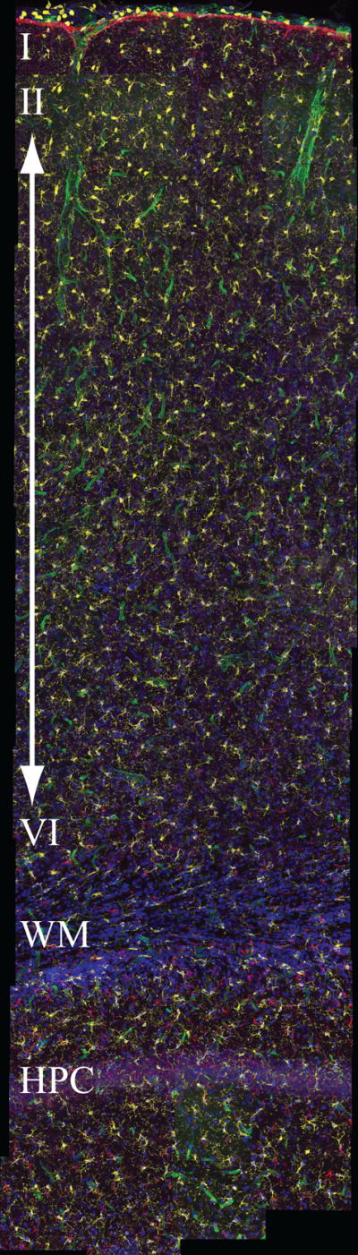
Maximum intensity projection of the montage of Dataset #2 taken from the rat cerebral cortex. The montage is 4,786×13,776×68 voxels in size. The five channels display: microglia in yellow, astrocytes in red, neurons in purple, vessel laminae in green, and nuclei in blue. The montage covers an entire strip of cerebral cortex, extending into corpus callosum and hippocampus.

Figure 11.

An example of accurate alignment of images around an electrode insertion site with very different magnifications. The dark hole in the center is indicative of the insertion site. The two separate images were taken using a 20× objective (0.9NA) with a zoom of 1.0 and 2.5 equaling a final magnification of 20× and 50×. (A) The 20× image of size 1,024×1,024×106, covering a tissue volume of 772×772×85μm³ (B) The 50× image of size 1,024×1,024×148, covering a tissue volume of 310×310×89μm³. (C) The result of registration. The 50× image shown in red is transformed to the space of the 20× image shown in green. The insertion site in yellow shows accurate alignment of the two images.

Table II summarizes measurements from the pair-wise registration (Step 1) on all distinct image pairs for the three datasets. Overall, less than 9% of all the image pairs tested in the two datasets overlap. The pair-wise registration step correctly and automatically eliminated 99.8% of pairs that do not overlap, and correctly registered 93% that do overlap. If we consider only images with an overlap greater than 7%, the success rate is 100%. The average NC errors were very small (< 0.05). Figure 8 shows 3 scatter plots summarizing the results of pair-wise registration (Step 1). Each data point in these scatter plots corresponds to an image pair. The NC error is plotted for each data point as a function of the image overlap (these overlaps are estimated from the validated joint registrations (Step 2), that are known to be accurate and reliable). The horizontal green lines indicate automatically estimated threshold values – data points below this threshold are declared as successful pair-wise registrations (indicated in black). Data points with NC error of 1 correspond to image pairs that overlap but failed to register on a pair-wise basis (indicated in blue). Points with zero overlap indicate image pairs (indicated in red) that should have failed, but were not declared as failures by Step 1. Happily, these points were all correctly recognized as failures by the joint estimation (Step 2). The few points between the threshold line but below NC = 1.0 represent mis-registered image pairs. Happily again, Step 2 correctly rejected these pairs. The scatter plot for Dataset #3 has an error threshold of 0.15. However, the wider spread of errors for correctly registered pairs (compared to the other two datasets) can be explained by the less favorable imaging conditions that resulted in irregular (non-affine) image distortion for some image pairs.

Figure 8.

Summary of registration and self-diagnosis performance as a function of image overlap. The NC is plotted for the 3 datasets in Tables I and II. Each data point in these scatter plots corresponds to an image pair. The horizontal lines indicate automatically estimated threshold values – data points above this threshold are declared failures by the joint registration (Step 2). Data points with NC error of 1 correspond to image pairs that overlap but fail to register. Points with zero overlap indicate image pairs that should have failed. (A) The scatter plot for Dataset #1 with the error threshold equal to 0.28. (B) The scatter plot for Dataset #2 with the error threshold equal to 0.16. (C) The scatter plot for Dataset #3 with the error threshold equal to 0.15. The wider spread of the errors for correctly registered pairs below the threshold value can be explained by the less favorable imaging conditions that result in irregular (non-affine) image distortion for some image pairs.

We next present visual examples illustrating aspects of our method. Figure 3A shows a 4-image montage from the upper-left region of Dataset #2 that was constructed based on pair-wise registration alone. The blue box indicates the image that was used as the anchor. The regions indicated by the red ellipses show significant alignment errors (largely attributable to the low overlaps). However, the joint registration results in Figure 3B show negligible alignment errors. In this example, the only image pair that does not have a transformation is the two images outlined in blue due to very low overlap. Figure 9 shows the only incorrect alignment from Dataset #2. Due to the complexity of the images (more channels that are rich in terms of cues), the second dataset has fewer incorrect alignments compared to the first dataset that has only two channels containing mostly blob shaped objects.

Figure 9.

The only instance of incorrect alignment from the Dataset #2, that was however, correctly detected as a registration failure automatically by the joint registration (Step 2). (A, B) The original images. (C) Registration results displayed by projecting the image in Panel A in red, and the Panel B in green. The NC error for this image pair is 0.28 pixels (>0.16), and is correctly recognized as an outlier in the joint registration.

We next examined our algorithm’s performance on images with deficient staining. While every histologist strives to produce tissue staining of impeccable quality, the practical reality is that imperfect staining does occur. Issues such as high background staining (uniform, but relatively low-level, staining of tissue components not of interest), or physical retention of staining molecules in aggregates within the tissue leading to a “noisy” image are commonplace, and for many research questions small amounts of staining imperfections are acceptable provided the signal of interest is not obscured. A range of imperfections exist for any given histological staining procedure that do not prevent a human observer from accurately interpreting the content of the stained image, and would therefore not require a second attempt at staining. Thus, for many researchers, one measure of quality of an automated method is its ability to produce an accurate output for input images at the margin of acceptable image quality produced in the laboratory. During testing of our algorithms, image sets that varied in background staining across individual confocal stacks were tested. The inconsistency in the background staining has no effect on initialization in the x – y plane since the extraction of corners and edges in Step 1 is robust to fluorescence signal variations. For refinement of the 3-D transformation, normalized cross-correlation is also designed to be robust under linear illumination changes. This is illustrated in Figure 10. The nuclear channel is displayed in blue and the neuronal channel in green. The confocal stack in panel A contains higher background staining when compared to the adjacent stack in panel B. The arrows indicate the corresponding areas in the two image stacks. Panel C shows a close-up of the montage of the neuronal channel. It demonstrates accurate alignment using the neuronal channels with neurons from A in green and neurons from B in red. When the two images are well aligned, the neurons in the overlap area correctly appear yellow, as seen here.

Figure 10.

Illustrating successful registration of images with problematic staining. The nuclear channel is in blue and the neuronal channel in green. The confocal stack in A contains higher background staining when compared to the adjacent stack in B. The arrows indicate the corresponding areas in the two image stacks. C is a crop of the montage of the neuronal channel. It demonstrates accurate alignment using the neuronal channels with neurons from A in green and neurons from B in red. When the two images are well aligned, the neurons in the overlap area correctly appear yellow, as seen here. Images in this figure are from dataset #1.

Next, we tested our algorithm on Dataset #3 that was taken under less ideal conditions. During image acquisition for Dataset #3, immersion oil that was contaminated with water was inadvertently used, and the last few collected confocal stacks show spatial distortions between optical slices within each stack. As one moves from one optical slice to the next, neuronal nuclei can be seen to shift in the x – y plane large distances relative to the small thickness (0.7 microns) of the optical slices (Figure 7A). This effect is not uniform between optical slices of a stack or within any individual optical slice; for instance, if one compares the left side of the three optical slices in panel A to the right side, one can see that the x – y shifts are greater for the left compared to the right. Thus there is no systematic transformation of the pixel information in the x – y plane. Despite this distortion of individual confocal stacks, the montage synthesis was successful (Figure 7C). Since this distortion is better appreciated when the user can move down through the z planes, a tif image containing the 3 planes indicated in Figure 7 (named Figure7Asupp.tif) has been included in the supplementary materials which can be opened in Irfanview or ImageJ.

The algorithm was also effective at aligning images of very different magnifications. Figures 11A & B are example images showing the microglia at an electrode insertion site. A single shank device was implanted into the neocortex of an adult Sprague-Dawley rat. Two maximum intensity projection micrographs from the same sample show reactive astrocyte distribution one week after device insertion. The dark hole within the center of the projection is indicative of the insertion site. The 3D confocal images were collected on a Leica TCS SP5 scanning confocal microscope. Two separate images were taken using a 20× objective (0.9NA) with a zoom of 1.0 and 2.5 equaling a final magnification of 20× and 50×. The transformation was accurately estimated in the x-y plane because the SIFT descriptors of the Lowe key points are scale-invariant. This property allows correct matching across scales. As seen from the seamless 2-color montage in Figure 11C, where the 50× image (displayed in red) is transformed to the space of the 20× image (displayed in green). The overlapping region appearing yellow shows accurate alignment of the two images, especially as evident in the processes of the microglia.

Overall, the methods described here are quite practical to use on common laboratory computers (Windows, Apple, Linux). Using a personal computer with a 2.94GHz Intel CPU and 12 GB of RAM, an image pair from Dataset #1 took about 15 seconds and a pair from Dataset #2 took about 60 seconds to register. For both datasets, the joint registration took a total of 10 seconds. If only considering the 4-neighbor adjacent pairs, the Dataset #1 and Dataset #2 took 40 and 130 minutes, respectively.

VI. Discussion and Conclusions

This work grew out of a real need to investigate problems in neuroscience that require analysis of fine sub-cellular details over extended tissue regions at the same time, problems that can only be addressed by step-and-repeat 3-D microscopy, and not by lower-resolution methods such as magnetic resonance imaging. Such questions include how neurons are organized into a layered architecture within the cerebral cortex; which neuronal populations form activated neural circuits during specific behaviors; how to map networks of gene expression involved in learning and memory; and how to characterize the cellular patterns of response to tissue injury following electrode or neuroprosthetic device implantation, as a function of distance from the implantation site. While these motivating problems are in the field of neurobiology, the innate generality of our algorithm design makes it useful to microscopists in other disciplines as well. These needs exist despite the advances over the past decade in microscopy instrumentation.

The net result of our advances is to make automated 3-D registration and mosaic synthesis accurate, robust, scalable, accessible, and usable for microscopy. By using a combination of feature- and intensity-based methods, generic features, robust estimation methods, design for low image overlaps, and globally-consistent alignment, the current method is useful to any microscopist working with image tiles regardless of the nature of the stained object or tissue. Highlights of our method include the fully “hands-free” automation without the need for careful adjustment of parameter settings, the benefit of automatic self-diagnosis of invalid registrations, and computational efficiency. These features make our approach inherently scalable for larger datasets.

Table III.

Results of pair-wise registration running on all distinct image pairs from the three datasets listed in Table II. The normalized cross-correlation error (NC) is dimensionless.

	# Pairs with overlap	# Registered pairs	# Incorrectly registered pairs	# Incorrectly failed pairs	Average NC error	NC Error threshold	Mean time per pair (sec)
Dataset #1	198	188	6	9	0.05	0.28	15
Dataset #2	145	131	1	14	0.03	0.16	60
Dataset #3	110	102	18	8	0.03	0.15	15

References

- Al-Kofahi O, Can A, Lasek S, Szarowski DH, Turner JN, Roysam B. Algorithms for accurate 3D registration of neuronal images acquired by confocal scanning laser microscopy. J Microsc. 2002;211:8–18. doi: 10.1046/j.1365-2818.2003.01196.x. [DOI] [PubMed] [Google Scholar]
- Appleton B, Bradley AP, Wildermoth M. Towards optimal image stitching for virtualmicroscopy. Digital Image Computing: Techniques and Applications. 2005:299–306. [Google Scholar]
- Bajcsy P, Lee S-C, Lin A, Folberg R. Three-dimensional volume reconstruction of extracellular matrix proteins in uveal melanoma from fluorescent confocal laser scanning microscope images. J Microsc. 2006;221:30–45. doi: 10.1111/j.1365-2818.2006.01539.x. [DOI] [PMC free article] [PubMed] [Google Scholar]
- Beck JC, Murray JA, Willows D, Cooper MS. Computer-assisted visualizations of neural networks: expanding the field of view using seamless confocal montaging. J Neurosci Methods. 2000;98:155–163. doi: 10.1016/s0165-0270(00)00200-4. [DOI] [PubMed] [Google Scholar]
- Becker D, Ancin H, Szarowski D, Turner JN, Roysam B. Automated 3-D montage synthesis from laser-scanning confocal images: application to quantitative tissue-level cytological analysis. Cytometry. 1996;25:235–245. doi: 10.1002/(SICI)1097-0320(19961101)25:3<235::AID-CYTO4>3.0.CO;2-E. [DOI] [PubMed] [Google Scholar]
- Bjornsson CS, Lin G, Al-Kofahi Y, Narayanaswamy A, Smith KL, Shain W, Roysam B. Associative image analysis: a method for automated quantification of 3D multi-parameter images of brain tissue. J Neurosci Methods. 2008;170:165–178. doi: 10.1016/j.jneumeth.2007.12.024. [DOI] [PMC free article] [PubMed] [Google Scholar]
- Brown LG. A survey of image registration techniques. ACM Computing Surveys. 1992;24:325–375. [Google Scholar]
- Can A, Stewart C, Roysam B, Tanenbaum H. A feature-based algorithm for joint linear estimation of high-order image-to-mosaic transformations: Mosaicing the curved human retina. IEEE Trans Pattern Anal Mach Intell. 2002;24:412–419. [Google Scholar]
- Capek M, Bruza P, Janacek J, Karen P, Kubinova L, Vagnerova R. Volume reconstruction of large tissue specimens from serial physical sections using confocal microscopy and correction of cutting deformations by elastic registration. Microsc Res Tech. 2009;72:110–119. doi: 10.1002/jemt.20652. [DOI] [PubMed] [Google Scholar]
- Capek M, Krekule I. Alignment of adjacent picture frames captured by a CLSM. IEEE Trans Inf Technol Biomed. 1999;3:119–124. doi: 10.1109/4233.767087. [DOI] [PubMed] [Google Scholar]
- Choe TE, Cohen L. Registration of multimodal fluorescein images sequence of the retina. Tenth IEEE International Conference on Computer Vision; Beijing, China. 2005. [Google Scholar]
- Chow SK, Hakozaki H, Price DL, Maclean NAB, Deerinck TJ, Bouwer JC, Martone ME, Peltier ST, Ellisman MH. Automated microscopy system for mosaic acquisition and processing. J Microsc. 2006;222:76–84. doi: 10.1111/j.1365-2818.2006.01577.x. [DOI] [PubMed] [Google Scholar]
- Emmenlauer M, Ronneberger O, Ponti A, Schwarb P, Griffa A, Filippi A, Nitschke R, Driever W, Burkhardt H. XuvTools free fast and reliable stitching of large 3D datasets. J Microsc. 2009;233:42–60. doi: 10.1111/j.1365-2818.2008.03094.x. [DOI] [PubMed] [Google Scholar]
- Feldmar J, Declerck J, Malandain G, Ayache N. Extension of the ICP algorithm to nonrigid intensity-based registration of 3d volumes. Comput Vis Image Underst. 1997;66:193–206. [Google Scholar]
- Fischler MA, Bolles RC. Random sample consensus: a paradigm for model fitting with applications to image analysis and automated cartography. CACM. 1981;24:381–395. [Google Scholar]
- Gholipour A, Kehtarnavaz N, Briggs R, Devous M, Gopinath K. Brain functional localization: a survey of image registration techniques. IEEE Trans Med Imaging. 2007;26:427–451. doi: 10.1109/TMI.2007.892508. [DOI] [PubMed] [Google Scholar]
- Gracias N, Santos-Victor J. Underwater video mosaics as visual navigation maps. Comput Vis Image Underst. 1999;79:66–91. [Google Scholar]
- Guzowski JF, Timlin JA, Roysam B, McNaughton BL, Worley PF, Barnes CA. Mapping behaviorally relevant neural circuits with immediate-early gene expression. Curr Opin Neurobiol. 2005;15:599–606. doi: 10.1016/j.conb.2005.08.018. [DOI] [PubMed] [Google Scholar]
- Higuchi K, Hebert M, Ikeuchi K. Building 3-d models from unregistered range images. Graph Models Image Process. 1995;57:315–333. [Google Scholar]
- Hill DL, Batchelor PG, Holden M, Hawkes DJ. Medical image registration. Phys Med Biol. 2001;46:1–45. doi: 10.1088/0031-9155/46/3/201. [DOI] [PubMed] [Google Scholar]
- Hsu L-Y, Loew MH. Fully automatic 3D feature-based registration of multimodality medical images. Image Vis Comput. 2001;19:75–85. [Google Scholar]
- Hsu W-Y, Poon W-FP, Sun Y-N. Automatic seamless mosaicing of microscopic images: enhancing appearance with colour degradation compensation and wavelet-based blending. J Microsc. 2008;231:408–418. doi: 10.1111/j.1365-2818.2008.02052.x. [DOI] [PubMed] [Google Scholar]
- Ibanez L, Schroeder W, Ng L, Cates J. The ITK Software Guide: The Insight Segmentation and Registration Toolkit. Kitware Inc; 2003. [Google Scholar]
- Maintz JB, Viergever MA. A survey of medical image registration. Medical Image Analysis. 1998;2:1–36. doi: 10.1016/s1361-8415(01)80026-8. [DOI] [PubMed] [Google Scholar]
- Jenkinson M, Smith S. A gobal optimization method for robust affine registration of brain images. Med Image Anal. 2001;5:143–156. doi: 10.1016/s1361-8415(01)00036-6. [DOI] [PubMed] [Google Scholar]
- Johnson A, Hebert M. Surface matching for object recognition in complex 3-dimensional scenes. Image Vis Comput. 1998;16:635–651. [Google Scholar]
- Karen P, Jirkovska M, Tomori Z, Demjenova E, Janacek J, Kubinova L. Three-dimensional computer reconstruction of large tissue volumes based on composing series of high-resolution confocal images by GlueMRC and LinkMRC software. Microsc Res Tech. 2003;62:415–422. doi: 10.1002/jemt.10405. [DOI] [PubMed] [Google Scholar]
- Lester H, Arridge SR. A survey of hierarchical non-linear medical image registration. Pattern Recognit. 1998;32:129–149. [Google Scholar]
- Lowe D. Distinctive image features from scale-invariant keypoints. Int J Comput Vis. 2004;60:91–110. [Google Scholar]
- Makela T, Clarysse P, Sipila O, Pauna N, Pham QC, Katila T, Magnin IE. A review of cardiac image registration methods. IEEE Trans Med Imaging. 2002;21:1011–1021. doi: 10.1109/TMI.2002.804441. [DOI] [PubMed] [Google Scholar]
- Maes F, Collignon A, Vandermeulen D, Marchal G, Suetens P. Multimodality image registration by maximization of mutual information. IEEE Trans Med Imaging. 1997;16:187–198. doi: 10.1109/42.563664. [DOI] [PubMed] [Google Scholar]
- Miller JV, Stewart CV. MUSE: Robust surface fitting using unbiased scale estimates. Proc IEEE Comput Soc Conf Comput Vis Pattern Recognit 1996 [Google Scholar]
- Oberlaender M, Bruno RM, Sakmann B, Broser PJ. Transmitted light brightfield mosaic microscopy for three-dimensional tracing of single neuron morphology. J Biomed Opt. 2007;12:064029. doi: 10.1117/1.2815693. [DOI] [PubMed] [Google Scholar]
- Preibisch S, Saalfeld S, Tomancak P. Globally optimal stitching of tiled 3D miscroscopic inage acquisitions. Bioinformatics. 2009;25:1463–1465. doi: 10.1093/bioinformatics/btp184. [DOI] [PMC free article] [PubMed] [Google Scholar]
- Price DL, Chow SK, Maclean NA, Hakozaki H, Peltier S, Martone ME, Ellisman MH. High-resolution large-scale mosaic imaging using multiphoton microscopy to characterize transgenic mouse models of human neurological disorders. Neuroinformatics. 2006;4:65–80. doi: 10.1385/NI:4:1:65. [DOI] [PubMed] [Google Scholar]
- Slamani M-A, Krol A, Beaumont J, Price RL, Coman IL, Lipson ED. Application of phase correlation to the montage synthesis and three-dimensional reconstruction of large tissue volumes from confocal laser scanning microscopy. Microsc Microanal. 2006;12:106–112. doi: 10.1017/S143192760606017X. [DOI] [PubMed] [Google Scholar]
- Stewart CV, Tsai C-L, Roysam B. The dual-bootstrap iterative closest point algorithm with application to retinal image registration. IEEE Trans Med Imaging. 2003;22:1379–1394. doi: 10.1109/TMI.2003.819276. [DOI] [PubMed] [Google Scholar]
- Sun C, Beare R, Hilsenstein V, Lackway P. Mosaicing of microscope images with global geometric and radiometric corrections. J Microsc. 2006;224:158–165. doi: 10.1111/j.1365-2818.2006.01687.x. [DOI] [PubMed] [Google Scholar]
- Thevenaz P, Unser M. User-friendly semiautomated assembly of accurate image mosaics in microscopy. Microsc Res Tech. 2007;70:135–146. doi: 10.1002/jemt.20393. [DOI] [PubMed] [Google Scholar]
- Viola P, Wells WM., III Alignment by maximization of mutual information. Int J Comput Vis. 1997;24:137–154. [Google Scholar]
- Yang G, Stewart CV, Sofka M, Tsai C-L. Alignment of challenging image pairs: refinement and region growing starting from a single keypoint correspondences. IEEE Trans Pattern Anal Mach Intell. 2007;23:1973–1989. doi: 10.1109/TPAMI.2007.1116. [DOI] [PubMed] [Google Scholar]
- Zitova B, Flusser J. Image registration methods: a survey. Image Vis Comput. 2003;21:977–1000. [Google Scholar]
Associated Data
This section collects any data citations, data availability statements, or supplementary materials included in this article.