High throughput, detailed, cell-specific neuroanatomy of dendritic spines using microinjection and confocal microscopy

Abstract

Morphological features such as size, shape and density of dendritic spines have been shown to reflect important synaptic functional attributes and potential for plasticity. Here we describe in detail a protocol for obtaining detailed morphometric analysis of spines using microinjection of fluorescent dyes, high resolution confocal microscopy, deconvolution and image analysis using NeuronStudio. Recent technical advancements include better preservation of tissue resulting in prolonged ability to microinject, and algorithmic improvements that compensate for the residual Z-smear inherent in all optical imaging. Confocal imaging parameters were probed systematically for the identification of both optimal resolution as well as highest efficiency. When combined, our methods yield size and density measurements comparable to serial section transmission electron microscopy in a fraction of the time. An experiment containing 3 experimental groups with 8 subjects in each can take as little as one month if optimized for speed, or approximately 4 to 5 months if the highest resolution and morphometric detail is sought.

INTRODUCTION

Spines are submicron-sized protrusions from dendritic branches and constitute the main sites of excitatory synaptic transmission in the brain. Time-lapse imaging in vivo has revealed that spines are, and remain throughout adulthood, highly motile structures (for reviews see^{1, 2}). Changes in size, shape and number of spines have been found in response to a large number of stimuli such as electrophysiological manipulations, learning, sensory enrichment or deprivation, and numerous disease models (for reviews see^2–8). Our laboratory has explored changes in spine size and number in animal models of stress, aging and menopause using single cell microinjections for two decades. In recent collaborative work, we have also explored spine changes in models of fear conditioning, depression and addiction.

Our first study using single cell microinjections with Lucifer Yellow was published in 1990⁹. At the time, our protocol was in its infancy and our analysis was restricted to neuronal morphology. Over the following decade and a half we slowly built upon this technique to incorporate dendritic density quantification by marking spines in manual 3D reconstructions of neurons under epifluorescence^10–12. Deconvolution (see Box 1) was added to our protocol as we began to obtain high resolution confocal z-stacks¹³ and our first spine size data were obtained using painstaking manual measurements of the head diameters and neck lengths of over 25,000 spines^{14, 15}. In 2008, following a longstanding collaboration with a computational group dedicated to the development of automated spine analysis techniques (see discussion below), we published our first study using NeuronStudio to semi-automatically quantify spine density and morphology¹⁶.

Box 1. Sources of uncertainty in confocal microscopy.

Images obtained with a confocal microscope suffer from a number of important physical limitations. Although some of these limitations can be compensated for by post-hoc image analysis, it is important to demarcate the exact capabilities of the methods used in this protocol. For a thorough examination of sources of uncertainty in a confocal system, we recommend the Handbook of Biological Confocal Microscopy⁴².

Uncertainty due to the wave nature of light

Point Spread Function

Objects imaged by a confocal microscope are convolved (i.e. distorted) by a complex pattern called the Point Spread Function (PSF). One of the main components of the PSF is the diffraction pattern resulting from light passing through a small aperture, which in the case of the confocal microscope is the pinhole. At its simplest description, the PSF can be described as a blurry sphere in the lateral direction (called an Airy disk), and a smeared ovoid in the axial direction.-In practice, the PSF can be measured by imaging an object that is smaller than the resolution limit. The top panels in the figure below depict the lateral and axial PSF when a 100 nm fluorescent bead with 560/580 nm excitation and emission peaks is imaged with our confocal setup with cubic voxels of 50 nm using a 100X 1.4NA oil immersion objective. Using the standard measurement for the size of an object in fluorescent images – the full width at half maximum (FWHM) intensity (yellow arrows in the figure below) – the bead has a lateral diameter of 280 nm and an axial diameter of 670 nm. For comparison, the sphere in the lower right corner of each panel in the figure below is 100 nm in diameter, i.e. the size of the actual bead. Consequently, all objects smaller than the PSF will appear exactly 280 nm in their XY diameter and 670 nm in their Z diameter. Using the formula for an ovoid,

$$\text{Volume}=\frac{4}{3}\pi ({{\text{r}}_{\text{XY}}}^2{\text{r}}_{\text{Z}})$$ (1)

our minimum resolvable volume is 0.028 μm³.

Deconvolution

The above calculated size of the smallest resolvable object in our confocal system is a serious limitation considering that the average dendritic spine in the CA1 region of the hippocampus has a head volume of 0.038 μm³ (see Anticipated Results). Can resolution be improved? Yes, by several methods, the most commonly employed one being post-hoc deconvolution. Deconvolution (available commercially and as open sourceat http://rsb.info.nih.gov/ij/plugins/fftj.html and http://cirl.memphis.edu/cosmos) is a computationally intensive image processing technique that improves contrast and resolution. Blind deconvolution is the preferred mathematical algorithm, as it first estimates the PSF from the image by calculating the blurring in all three dimensions, meaning that it can theoretically compensate for other optical aberrations present. Of the many deconvolution software packages available, we empirically found AutoDeblur (Media Cybernetics) to be the best. The bottom panels in the figure below show the same bead following deconvolution with AutoDeblur. The FWHM has been reduced to 180 nm laterally and 390 nm axially, resulting in a new minimum resolvable volume of 0.0066 μm³, which is only about twice the volume of the smallest spine head measured by ssTEM⁴³. Auspiciously, in rat CA1, only about 1% of spines have head volumes below this resolution limit (Hu and Chklovskii, personal communication).

Uncertainty due to the quantum nature of light

Shot noise

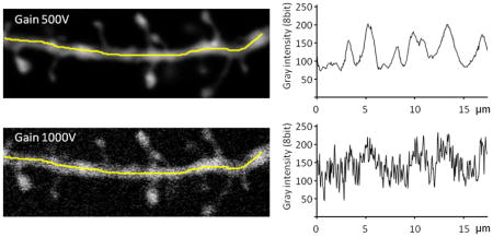
In a high quality, well-aligned confocal microscope the only noteworthy source of noise is that arising from the stochastic nature of photons. When the sample is really bright this is not an issue; however, when high gains are necessary to reach dynamic range (only a few pixels of minimum intensity and a few pixels of maximum intensity), this becomes detrimental to image quality. At a gain of 500V, a fully saturated pixel represents about 2000 photons, while at 1000V only about 11 photons are needed to reach saturation⁴⁴. Because of the quantal nature of light, the number of detected photons during a particular time interval varies around a mean and exhibits Poisson statistics, just like a coin toss experiment. Because in Poisson statistics the mean is equal to the variance, the lower the sample size, the more uncertainty exists about the outcome. Getting 3 heads out of 10 coin tosses does not necessarily mean that the coin is unfair, but getting 300 heads out of 1000 tosses will make anybody suspicious; yet in both cases there is an average outcome of 30% heads.

In order to quantify the shot noise in our system, which is defined as the standard deviation of the fluctuations in photon number, we used the root mean squared deviation (RMSD) between adjacent pixels along the dendrite, calculated as follows:

$$\text{RMSD}=\sqrt{{\sum }_i^n{(x_{1i}-x_{2i})}^2/n}$$ (2)

where x_{1 i} and x_2i are adjacent voxels and n is the total number of consecutive pixels analyzed.

As illustrated by both images and plots in the figure below, there is a significant increase in the fluctuation of the gray scale intensity along the dendrite when the gain is increased (achieved here experimentally by decreasing the power of the laser). The poor image quality when the shot noise is high is a serious problem when deciding what is and what is not a spine, both for the experimenter doing manual counts, as well as for NeuronStudio. Therefore, all measures should be taken to maximize the brightness of the sample, which is the main method to reduce the shot noise in the final image. If imaging a weakly stained neurite can’t be avoided, then methods that increase photon counting should be employed, such as increasing averaging and using longer scan times.

Spherical aberrations

Spherical aberrations result from differences in refraction and reflection of light rays striking the center versus periphery of an object when light travels through a spherical lens. In confocal microscopy, these spherical aberrations can be amplified by several factors that the experimenter has control over (discussed below). In a nutshell, as a result of spherical aberrations, objects deep within the tissue (and therefore far from the coverslip) will both appear less bright and be more blurred relative to objects closer to the coverslip. Because dendrites are found at varying focal depths, this can potentially lead to systematic bias of spine size data.

For the purpose of this protocol, we will restrict our discussion to narrowly defining spherical aberrations as resulting from one of two common mistakes: the use of the wrong coverslip thickness and mismatches in the refractive index (RI) of the immersion versus mounting media. However, it should be noted that some amount of spherical aberration is inherent to all objective types and a careful examination of the distortion under optimal conditions in your own system is very important for the determination of the range of depths at which dendrites should be imaged (see Experimental Design).

Coverslip thickness

All major microscope manufacturers (e.g. Zeiss, Olympus, Nikon and Leica) exclusively produce objectives that are designed to be used with 170 μm thick coverslips, which corresponds to a #1.5 coverslip size. In spite of this, #1 coverslips are the most widely sold type (~150 μm thick), followed closely by #2 coverslips (~220 μm thick). When imaging at or near the resolution limit, the use of the wrong coverslip size will render the data uninterpretable due to large effects on both the PSF⁴⁵ as well as on spherical aberrations⁴². Importantly, even coverslips that are sold as #1.5 can vary by more than 10 μm from their nominal value, which can still introduce large and fluctuating spherical aberrations into the dataset. One solution is to use a commercially available electro-mechanical micrometer to measure each coverslip before use and discard all coverslips found to deviate by more than a few microns from 170 μm. Another solution is to restrict the coverslip choice to Zeiss #1.5 coverslips (Part # 474030-9000), which are proposed to be the most precise in terms of their adherence to the nominal thickness.

RI mismatches

Each objective has a technical specification as to the immersion media that it was designed for, i.e. oil, water, air, or glycerol (although multi-immersion objectives also exist). Consequently, an oil objective for example, will only function ideally when all light going though it travels via media that is of the same RI as oil (1.52). Since the RI of the glass of the coverslip is also 1.52, in the case of oil objectives the problem begins at the interface between the coverslip and the mounting media. Mounting media with RIs close to 1.52 exist (e.g. DPX), but these usually require dehydration of the tissue, which is not desirable when precise size measurements will be attempted. For a variety of reasons, we have chosen VectaShield mounting media which has an RI of 1.46 and which therefore by definition will result in an increase in spherical aberrations. Whatever your objective may be, it is imperative that you try to match the RI of the immersion media, coverslip and mounting media to the specifications of the objectives as closely as possible. (For example, use a “Cytop” – a new type of coverslip with a RI of 1.34 – with a water immersion objective.) Unfortunately, it should be noted that even in cases in which the RIs of the media are matched perfectly, spherical aberrations will still exist, resulting from refractive differences in the specimen itself⁴²; for example, the RI of brain matter ranges from 1.40 to 1.47. Therefore, empirical determination of the magnitude of spherical aberrations in your setup and preparation is imperative in order to make an informed decision about the range of depths at which to image spines at high resolution (see Experimental Design).

Most recently, using the complete protocol described here, the quality of our morphometric data allowed us to parcel out an incredibly detailed view of the aging process in the prefrontal cortex of monkeys, where we found a dramatic loss of a particular morphologic subtype of thin spines¹⁷. We further showed that the remaining thin spines are shifted toward bigger sizes, potentially reflecting a loss of spine turnover, which has been shown to decrease in rodent aging cortex by two-photon time-lapse imaging¹⁸. Most interestingly, the mean volume of the remaining thin spines was highly significantly correlated with the cognitive status of the animal, while the volume of the unchanged mushroom spines showed no correlation to any behavioral index¹⁷.

Thus far, in our laboratory and in collaboration with other groups^{16, 19–21} we have used the current protocol in animal models ranging from rodent to monkey and brain areas as diverse as the prefrontal cortex, hippocampus, amygdala and nucleus accumbens. All models and regions we have tried thus far have been amenable to microinjection. However, it is conceivable that areas we do not have any experience with, such as brain stem and spinal cord, might not be amenable to microinjection.

The reliability and validity of this protocol can also be construed from the various other groups around the world who have published spine density and size data following microinjections with dyes such as Lucifer Yellow²², Alexa 488²³ and Alexa 594^24–26. Importantly, the parallel development of similar protocols in other laboratories points to a great degree of versatility in the necessary equipment. Confocal microscopes previously used range from Zeiss (in our own work), to Olympus²³, to Leica^24–26, to BioRad²²; objectives used range from 100x oil-immersion lenses with NA 1.4^{17, 22}, to a 63x water-immersion lens with NA 1.2²³ and a 63x glycerol-immersion lens with NA 1.3^24–26. Most commonly, 3D spine density data has previously been acquired by manual tracing of dendrites combined with marking of spines as they appear into view using software such as Imaris²², NeuroLucida^24–26 or Metamorph²³, while spine size data has been acquired with manual identification of spines followed by semi-automatic measurements using software such as Metamorph²³ or Imaris^{22, 24–26}.

Z-smear correction for accurate spine volumetric data

The crucial component that revolutionized our ability to conduct high-throughput, high resolution analysis of dendritic spines has been the computational innovation that led to automated spine-detection algorithms. Our laboratory currently exclusively uses NeuronStudio^{27, 28}, which is available for free download at http://research.mssm.edu/cnic/tools-ns.html. This program employs Rayburst Sampling, which very precisely identifies and measures the volume of objects from Z-stacks by casting a large number of “rays” from the center of mass of a 3D object to its surface^{27, 28}. This results in pyramids of volume (space contained between three adjacent rays), which are then used to precisely compute the volume and surface area of the object, irrespective of its shape. However, although the Rayburst algorithm accurately describes the volume of the spines in an image, it does not accurately describe the volume of the original spine, since one of the major drawbacks of confocal microscopy is a smear in the Z-direction (see Box 1).

Therefore, in order to circumvent this problem, we recently added a new function in NeuronStudio to mathematically compensate for the optical Z-smear. A correction factor is first computed heuristically by obtaining the ratio of the XY diameter of the dendrite to the diameter of the same branch in the Z-axis, adjusting for branch angle. The correction factor is then applied to the Z component of each ray used to calculate the Rayburst volume, effectively removing the Z-smear without affecting the shape or XY spread of the object. To illustrate, correcting the Z-smear for the fluorescent bead from Box 1 would force the axial full-width half maximum (FWHM) to 180 nm (i.e. matching the axial diameter to the lateral one), which would result in a new minimum resolvable volume of 0.003 μm³.

Fig. 1A shows the two-step resolution enhancement in our protocol, firstly by deconvolution with AutoDeblur (Media Cybernetics), which improves resolution laterally as well as axially, and secondly by Z-smear correction in NeuronStudio, which further adjusts the axial resolution with no effect laterally. For the 10 spines displayed in Fig. 1B, the average spine head volume is 0.104±0.015 μm³ in the raw confocal image, 0.053±0.006 μm³ in the deconvolved image and 0.032±0.003 μm³ following Z-smear correction (paired t-test p<0.001 for all comparisons). In a separate study of 114 spines from 7 dendrites, the Z-smear correction reduced the spine head volume by 35±1% (volume mean=0.053±0.003 μm³ without correction versus mean=0.034±0.002 μm³ with correction, data not shown). The percent decrease in volume varied a great deal among the spines, ranging from 14 to 78%, resulting from the fact that the correction is applied to the individual rays in the Rayburst, rather than globally. This allows the algorithm to maintain shapes (e.g. if a mushroom spine is ovoid it remains ovoid even after the correction) as well as ensures that other distances are not distorted; thus, neither dendritic length, spine head diameter, nor max spine length are affected by the Z-smear correction (data not shown).

Figure 1.

The final high-resolution image obtained by our methods results from a two-step improvement of the PSF by deconvolution followed by Z-smear correction. A. The lateral and axial views of a dendritic spine in a raw confocal image, after deconvolution and after the Z-smear correction. Note that while the deconvolution improves both the lateral as well as the axial resolution, the Z-smear correction is exclusively aimed at the axial distortion that remains even after optimal deconvolution. B. The two-step improvement in the 3D resolution is plotted for 10 spines (various colors) and their group average (black line). There is a 49% reduction in volume by deconvolution and a further 40% improvement by the Z-smear correction (paired t-test, p<0.001 for each step). Put another way, a spine in a raw confocal stack is on average 226% bigger than its actual volume (range 77–294% for the 10 spines shown here). Animal use in this experiment was conducted with strict adherence to our Institutional Animal Care and Use Committee.

Alternatives to microinjection

The most widely used technique for fast identification of cellular morphology throughout the past century has been the Golgi stain. However – although still widely used – this method only allows for 2D counts of spines. Constraints in the Z-resolution in widefield microscopy result in the detection of only about one-third of spines, with the remaining protrusions, located above or below their dendrite of origin, obscured. Additionally, it is difficult to use the Golgi stain to extract accurate measurements of spine size. The advent of confocal microscopy in the mid 20^th century made it possible to resolve 3D objects at the light level by the addition of a pinhole which rejects out of focus light. Since then, various methods of staining cells for confocal imaging have been employed in addition to microinjection, such as transgenic or viral delivery of fluorescent proteins²⁹ and Diolistics^30–32. Diolistics is traditionally viewed as being the easiest method to setup and perform. However, this technique results in very few complete, resolvable, individual neurons, due to a high degree of truncated neuronal segments and background staining. In addition, Diolistics is hard to combine with systematic studies of specific subpopulations of cells. Intracellular injections, on the other hand, can target very precise elements of circuits based on molecular attributes (e.g. transgenic mice expressing GFP in particular cell types¹⁹) or connectivity (using e.g. retrogradely labeled cells^{10, 33}).

Alternatives to confocal microscopy

The confocal system offers the highest resolution in diffraction-limited microscopy. However, in the past decade several new approaches have broken past the barrier of diffraction. Collectively known as “super-resolution,” some of these methods have realized resolutions on the order of nanometers; they include: structured illumination microscopy (SIM), stimulated emission depletion (STED), total internal reflection (TIRF), stochastic optical reconstruction microscopy (STORM) and photoactivated localization microscopy (PALM). A detailed discussion of these methods is beyond the scope of our protocol but is available elsewhere³⁴. Although these methods are noteworthy in that they offer the hope of one day achieving results superior to the confocal microscope in morphometric characterization of dendritic spines, they are at present neither widely available nor reasonably priced. In addition, there are more subtle disadvantages that should be considered prior to deciding on acquiring such a system for the purpose of imaging dendritic spines. TIRF for example, can only image the first 200 nm below the coverslip, rendering it useless in the setting of neuronal morphology. SIM, STED, STORM and PALM require significantly longer acquisition times than those necessary in confocal microscopy. In a recent study using STED microscopy to look at spines³⁵, pixel dwell time was reported to be 0.5–1 ms, which is up to 1000x slower than what we recommend in our protocol. Therefore, although super-resolution technology is enormously valuable in certain settings, such as subcellular localization of proteins³⁵, it is at present unclear what role it will play in morphometric analysis of dendritic spines.

Alternatives to NeuronStudio

To the best of our knowledge, the approach we employ with NeuronStudio^{27, 28}, including the addition of a Z-smear correction, is the first to give truly accurate spine volumetric measurements using fluorescent microscopy. However, in the past decade, several other programs aimed at automated spine identification have been developed (for review see³⁶), with Imaris Filament Tracer (Bitplane) offering one of the leading commercially available alternatives³⁰. However, to our knowledge, no other software has obtained data that is as closely correlated with serial section transmission electron microscopy (ssTEM) as NeuronStudio. For example, Imaris Filament Tracer suffers from the serious disadvantage of not having a way to define the spine head. As a result, the suggested alternative of spine terminal point volume, grossly underestimates the true spine volume. Although we have never used Imaris Filament in our own work, we briefly tested it on data from one animal in order to compare and contrast (animal 2 from Anticipated Results and Supplemental Fig. 1). The mean volume measured by NeuronStudio was 0.042±0.002 μm³, versus 0.019±0.002 μm³ measured by Imaris Filament (data not shown). This discrepancy is not merely a reflection of a scale-down in volumetric estimation, as normalizing the data still led to a significant difference in the distribution of head volumes (Kolmogorov-Smirnov test, p=2×10⁻²⁵, data not shown). Rather, it arises from the fact that in contrast to NeuronStudio, which uses the Rayburst algorithm to measure the entire extent of a spine head regardless of shape, Imaris Filament measures the minimum diameter of the terminal point and then computes the volume by simply plugging in this diameter into the formula for the volume of a sphere. As a result, Imaris Filament misses a great deal of the variability in volume that results from the biological diversity in spine shape, and this is reflected by a dramatic difference in the variance of the data obtained with the two programs (0.0016 μm⁶ for Imaris versus 0.0031 μm⁶ for NeuronStudio, data not shown).

The limitation described above pertains specifically to spine volumetric data, as our results in terms of spine density did not differ significantly between Imaris Filament and NeuronStudio; furthermore, in light of our admittedly limited experience with software other than NeuronStudio, the comparison is not meant to be comprehensive. Rather, we would like to suggest to the reader that a very careful analysis of potentially suitable software should be done prior to choosing one, and that methods outlined in this protocol will provide an excellent platform for evaluating any such software.

Strengths and limitations of the protocol

Presently, the most detailed anatomical measures of spines are performed with ssTEM. Although ssTEM offers an unparalleled look at connectomics³⁷, this is an exceedingly demanding and time-consuming technique, which has the additional limitation of being difficult to use when identification of specific subpopulations of neurons is desirable. Microinjection followed by high resolution confocal microscopy and post-hoc image analysis yields spine morphometric data in a fraction of the time. Furthermore, we now show that our protocol not only yields accurate 3D spine density counts, but – remarkably – also correctly captures spine head volumes (see Anticipated Results). While on an individual spine basis the precision of the volumetric measurement will remain uncertain until the same spines are imaged at both the light level and by ssTEM, the accuracy of averages and distributions derived from large datasets using the methods described in this protocol can comfortably be inferred based on the consistency of our data with previous results from the literature (see Anticipated Results).

The main limitation of this protocol is that the results are restricted to anatomy. Thus, unlike in studies using ssTEM, microinjection and fluorescent microscopy cannot for example confirm or deny the presence of a synapse. However, because most excitatory synapses in the brain occur on dendritic spines and because the vast majority of spines have been shown to have presynaptic partners³⁸, the quantification of these structures is highly relevant to brain circuitry. Of particular relevance to the present protocol is the evidence showing that spine volume is tightly correlated with postsynaptic density (PSD) size and number of AMPA receptors, which ultimately implies that spine volume reflects synaptic strength^{6, 39, 40}. In addition, spine head volume has been linked to relative plasticity and stability of spines in the context of cognitive performance^{2, 17}. The totality of structural findings from our work and others ultimately leads to a concept that has gained a lot of recent popularity^{4, 41}: namely, spine size can be thought of as a snapshot in time from which one can deduce something about the history of the circuit as well as its potential for future plasticity. As our data suggests, we can now use microinjection and confocal microscopy to evaluate synaptic plasticity in fixed tissue.

EXPERIMENTAL DESIGN

Tissue storage

One of the biggest drawbacks of microinjection has up until recently been the short time window during which the tissue is amenable to microinjection. Within one to two weeks tissue degradation begins to render cells unloadable, as evidenced by increasing leakage of dye and an inability to fill cells to their tips. This places a major constraint on the number of animals that can be included in a single experiment. We recently discovered however, that adding 0.1% sodium azide to the phosphate buffer can significantly prolong or even remove this time window. Fig. 2A shows an example of two sections from the same animal, loaded and imaged nine months apart. Our analysis of spine density (Fig. 2B), spine subtypes (Fig. 2C), and spine size (Fig. 2D), all indicated that there is no difference between the spines obtained with microinjection immediately after perfusion versus microinjection following prolonged storage. Because we serendipitously had monkey sections stored in phosphate buffer with sodium azide at 4 degrees from previous experiments, we were able to test even longer storage times and we successfully loaded tissue perfused up to 7 years prior. The removal of the time window for microinjection gives the experimenter additional to unlimited time to inject enough cells, and allows for going back to animals that are deemed important following the completion of other types of analysis (e.g. biochemistry, blood work, imaging, or behavior). It should be noted however, that prolonged storage only works well for well-perfused tissue. Therefore, prior to designing an experiment it is vital that the perfusion steps (Steps 2–6) are practiced until good tissue can be consistently obtained. Light fixations of less than an overnight in post-fixation might also not be amenable for storing. If light fixation is desired we recommend a pilot study to look at the effects of long-term storing.

Figure 2.

Microinjections can be performed immediately after or months to years following perfusion if tissue is stored in 0.1% sodium azide in PBS. A. Example of two CA1 sections from the same rat, microinjected and imaged nine months apart. No apparent loss of quality was observed in either the microinjection or the high resolution imaging. B. Spine density using fully automated NeuronStudio counts did not differ in four animals that were loaded either immediately after perfusion or nine months later (paired t-test, p=0.3). C, D. Neither subtype density nor subtype head diameter, plotted as means ± standard deviations, showed an interaction with storage condition (two-way ANOVA, p=0.5 and p=0.4, respectively). Animal use in this experiment was conducted with strict adherence to our Institutional Animal Care and Use Committee.

Sampling

All efforts should be made to obtain an unbiased sampling of spines. Picking the “best” spot should be avoided by creating very clear rules for choosing segments. Two such rules which we have employed in the past are:

1. Drawing concentric circles at known distances from the cell body (e.g. 60, 120, and 180 μm) and imaging all dendritic segments intersecting with the circles (e.g. in neocortex and nucleus accumbens)

2. Drawing lines at specific distances from the cell body layer (e.g. in CA1) or the pia (e.g. in neocortex) and imaging all dendrites intersecting with the lines

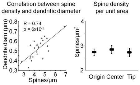
Additional rules we have used are: image only dendrites that are parallel with the section (because the time required to image dendrites that are transverse increases exponentially), avoid bifurcations, avoid first and last 10% of dendritic segments, and avoid large fluctuations in the dendritic diameter (as illustrated in Box 2, where we show a significant correlation between the dendrite diameter and spine density in rat CA1).

Box 2. Calculating spine density per unit surface area.

The large range in spine density in the male rat CA1 observed by us and others should be considered in the design and interpretation of results containing small sample sizes. Since the range within individual animals can be more than two-fold, an underpowered study comparing different experimental groups can easily result in false-positives. This is of particular importance in studies were it is not easily discernable what dendritic subcompartment is being imaged, which is often the case with diolistics, viral transfection, and other methods in which background is high and only a limited number of dendritic segments can be obtained. In order to evaluate whether the large variability in spine density could be compensated for in the final analysis, we looked at the correlation between spine density and dendritic diameter, noting that the beginning of neurites are on average thicker than the tips. Indeed, we found a very strong correlation (Pearson’s R=0.74, p = 6×10⁻⁵; see lefthand graph in the figure below), which led us to consider the effects of looking at the spine density per unit area rather than per unit length. For each dendrite, we computed its surface area by assuming it to be a cylinder and using the formula 2πr²+2πrh, where r is the mean radius of the dendrite (as reported by NeuronStudio) and h is the length. We then computed the density per unit area of each segment by dividing the number of spines by the surface area. This resulted in a much smaller range of values (mean 2.78±0.09 spines/μm², range 2.12–3.79 spines/μm²), perhaps indicating that spine number is scaled to the local amount of plasma membrane, and eliminated the difference between dendritic compartments (see righthand graph in the figure below; p>0.6 for all group comparisons). These data suggest that density per unit area of dendrite could be a useful normalization technique for underpowered studies, at least for the rat CA1 region.

In light of the large variability in spine density and spine size we have observed in several models (see Anticipated Results), we recommend sampling 5–10 animals per experimental group, 5–10 cells per animal and 5–8 segments per cell. If analysis will be conducted to look at differences between different cellular compartments, e.g. apical versus basal dendrites or proximal versus distal, it should be ensured that a minimum of 15 dendrites from each compartment are imaged. Statistics should be done by first averaging the dendrites from a cell, then averaging the cells in an animal, followed by averaging the animals in a group.

Range of depths appropriate for imaging

As outlined in Box 1, spherical aberrations can at times put severe limitations on the depths at which it is appropriate and/or feasible to image at high resolution. In order to test the effects of spherical aberrations in our system, we imaged 17 dendrites located at depths between 10 and 80 μm below the coverslip from two neighboring cells in monkey prefrontal cortex microinjected with Lucifer Yellow (Fig. 3). As expected, the gains necessary to reach dynamic range increased steadily at increasing focal depths and beyond about 80 μm it became unfeasible to image as a result of loss of intensity (see gains necessary to image each dendrite in Fig. 3A).

Figure 3.

Empirical evaluation of the effect of spherical aberrations on 2D and 3D resolution. A. Seventeen basal dendrites located 60 to 120 μm from the soma of two monkey prefrontal cortex layer III cells injected with Lucifer Yellow were imaged at varying focal depths. The figure shows the XZ views of a subset of neurites following deconvolution, placed at the anatomically correct depth from coverslip. The arrows point to the position and focal depth of the soma of each cell. The numbers next to each dendrite represent the gain necessary to image at full dynamic range. Beyond a focal depth of about 80 μm, the drop-off in intensity made it unfeasible to continue imaging since gains above 800V would have been necessary, leading to poor image quality. Scale bar=5 μm. B. Fully automatic NeuronStudio quantification of spine head diameter and spine head volume was performed on the same ~400 spines in raw confocal z-stacks (top), deconvolved z-stacks (middle), and using Z-smear correction on deconvolved z-stacks (bottom). Pearson’s correlations were used to evaluate the blurring effect as a function of focal depth. Spherical aberration has a significant effect on both 2D and 3D resolution in raw images (top). Deconvolution is able to compensate for the effect on 2D but not 3D resolution (middle). However, Z-smear correction extends the compensation to 3D resolution as well (bottom). All correlations were also run for the spines of each cell individually yielding very similar results (data not shown). Therefore, in our system and preparation, and using our post-hoc analysis techniques, the effect of spherical aberrations can be ignored at least up to a focal depth of 80 μm. Animal use in this experiment was conducted with strict adherence to our Institutional Animal Care and Use Committee.

We then conducted fully automated NeuronStudio analysis on the raw confocal z-stacks in order to evaluate the effect of spherical aberrations on 2D (spine head diameter) and 3D (spine head volume) resolution as applicable to our model, and found a significant – albeit small – blurring effect as a function of distance from the coverslip (Fig. 3B top graphs). Conducting the same analysis on deconvolved images showed that deconvolution can compensate for the blurring in 2D but not 3D (Fig. 3B middle graphs). Interestingly, when adding the Z-smear correction function to the deconvolved images, the effect of spherical aberrations in 3D also disappears (Fig. 3B bottom graphs). There was also no effect on spine density as a function of focal depth (Pearson’s correlation, p=0.61, data not shown).

In light of these data, we routinely image spines at focal depths of up 80 μm. However, we want to caution the reader that results could be very different in other systems and with other immersion and mounting media. The amount of spherical aberration and the ability of deconvolution and Z-smear correction to compensate for it should be carefully evaluated in your specific setup and preparation prior to deciding on the appropriate range of depths that dendrites can and should be imaged at.

Imaging parameters

The choice of imaging parameters will be based on experimental priority, quality of the material, the fluorophore used, and the available confocal system. While we offer a guide for how to choose parameters, please note that confocal systems and microscope optics differ quite a bit and we strongly recommend using our analysis below as a protocol for exploring your own system rather than as an absolute reference. Table 1 contains examples of two different sets of parameters we have used with our system, one designed for fast acquisition, the other designed for the highest resolution that we can obtain with our confocal microscope (see Anticipated Results for examples of data we have obtained with each of the two sets of parameters). In general, if the main interest is in spine density and relative size, very fast imaging can be employed; on the other hand, if accurate spine morphology is needed, slower imaging should be used. No matter what the choice, the same imaging parameters must be used for the entire study. In addition, all dendrites should be imaged at their dynamic range, meaning that the gain and offset should be adjusted such that in the final image only a few pixels are fully black (0 intensity) and only a few pixels, preferably in the dendrite and not the spines, are fully white (max intensity, e.g. 255 in an 8 bit image). Fig. 4 offers an overview of the effect on resolution in 2D (spine head diameter), resolution in 3D (spine head volume) and shot noise contributed by each imaging parameter in our system. The same spines were serially imaged while systematically changing the individual parameters. The data displayed in Fig. 4 is from rat CA1 dendritic segments. However, all experiments were also duplicated in monkey prefrontal cortex (where spines have on average 3–4 times bigger head volumes) yielding very similar results (data not shown).

Table 1.

Sample imaging parameters optimized for speed versus resolution.

Overview of two sets of parameters optimized for either speed or resolution in our confocal system. These parameters have been used for imaging LY filled cells with our Zeiss LSM 510 using an oil immersion 100x 1.4 NA objective and a 458 nm 30 mW Argon laser. Please note that these parameters cannot merely be applied to other systems, but rather are meant to serve as examples of successful application of the imaging principles described in this protocol.

Parameter	Optimization for speed	Optimization for resolution
Power	30%	10%
Raster size	1024×1024 (cropped to approx 1024×300)	512×512 (cropped to approx 512×200)
Zoom	2.5	3.3
Step size	0.3 μm	0.05 μm
Voxel size	33×33×300 nm3	50×50×50 nm3
Averaging	Line 4	Line 4
Speed	1.61 μs/pixel	6.39 μs/pixel
Average segment length	35±0.2 μm	26.5±0.2 μm
Time per segment	2–3 min	15–25 min

Figure 4.

Systematic analysis of the effect of imaging parameter choice on resolution and shot noise. Each parameter was varied in stepwise fashion and images of the same dendritic segment were acquired serially. Experiments were performed in both rat CA1 as well as in monkey prefrontal cortex, with both animal models yielding highly consistent results for all parameters, despite the large difference in spine size (monkey prefrontal cortex spines have heads that are 3–4x bigger in volume). Unless otherwise specifically varied, all imaging was performed at full dynamic range with 50×50×50 nm voxels, averaging of 4 frames, speed of 2 μs/pixel, and a pinhole of 1 AU. Column i provides an overview of how each parameter influences the delicate balance between efficiency and resolution. Examples of serially images spines are shown in column ii. All images in column ii (except Dii) were chosen from monkey prefrontal cortex where the lower spine density allows for easier visualization of individual spines. Spine head diameter and spine head volume was evaluated as a function of parameter only for spines automatically detected by NeuronStudio. Each color line in columns iii and iv represents a single spine from rat CA1, while the black lines represent the group averages. Shot noise, column v, was quantified in 2D images of dendrites using root mean square difference (RMSD) of gray scale intensity in consecutive pixels (see Box 1). In columns iii and v, the Y-scale was kept the same for easier comparison across experiments; this could not be achieved for column iv because of the large variability in volume resulting from changes in the sampling parameters. A. Gain has the biggest effect on shot noise (Av) and begins to affect the both the head diameter (Aiii) and the head volume (Aiv) above around 800V. All efforts should be made to optimize the microinjection technique so that images used for analysis have gains below about 750V. B. Averaging does not have an important effect on head diameter (Biii) and volume (Biv). In accordance with Poisson statistics, shot noise decreases proportionally to the square root of the number of frames averaged (Bv, red dotted line = theoretical decrease using Poisson statistics). However, averages of more than 4 frames are superfluous, and can negatively impact image quality if deconvolution is used (Bv, black dotted line). C. In good quality images of gains below 750V, imaging speed plays the least important role on 2D resolution (Ciii), 3D resolution (Civ), and shot noise (Cv). D. Decreasing the pinhole diameter can increase the resolution (Diii, Div), but is not practical unless extremely bright samples are used. This is because, when the pinhole aperture is minimized, less photons make it from the sample to the detector, which increases shot noise (Dv). For low gain applications (below 500V at 1 AU) such as the DAPI-stained epithelial nucleus shown in Dii, decreasing the pinhole diameter to 0.25 AU can improve resolution by 30%. E. Oversampling in the XY dimension increases the 2D resolution (Eiii), but decreases the 3D resolution (Eiv) if the size of the Z-step is kept the same, as was done here. This is due to the loss of voxel cubicity. Importantly, note that oversampling is actually a necessity for deconvolution to be capable of improving contrast (Ev). F. The use of cubic voxels is ideal for all applications in which imaging is followed by highly mathematical image analysis. The improvement in 2D resolution as a function of oversampling (Fiii) is now matched by a similar increase in 3D resolution (Fiv). Also note that when the Z-step is matched to the oversampling in the XY-dimension, deconvolution improves the contrast even more dramatically in response to decreasing voxel size (compare Ev with Fv, where the only difference is in Z-step). G. Although cubic voxels are decidedly the best for 3D resolution, keeping the Z-step close to the Nyquist optimal size can greatly speed up imaging without a change in 2D resolution (Giii). Furthermore, the spine head volumes change linearly as a function of Z-step size (Giv). This results in “volume scaling”, i.e. a tight correlation between individual spines’ head volumes at e.g. 50 nm versus 350 nm Z-step sizes (Gv). Consequently, although volumes measured from stacks with large step sizes are not accurate, meaningful comparisons among spines can still be performed. Animal use in this experiment was conducted with strict adherence to our Institutional Animal Care and Use Committee.

• Gain. Gain is the voltage applied in the photomultiplier (PMT) of the confocal detector in order to amplify the signal. A photon reaching the PMT is first converted into an electron and then at each of a number of steps amplified by a factor dependent on the voltage. The final number of electrons reaching the detector is then converted into a gray scale intensity value for the image. Gain is therefore a double-edge sword. On the one hand, higher gain is useful in allowing for identification of very dim samples. On the other hand, at higher gains, less photons are represented in the final image and therefore the image is of much poorer quality because of the increase in shot noise (see Box 1). The size of both spine head diameters (Fig. 4Aiii) and spine head volumes (Fig. 4Aiv) begin to show distortion at gains above 900V and 800V respectively, due to the inability of the deconvolution to fully compensate for the increase in shot noise (Fig. 4Av). The low (signal-to-noise ratio) SNR at high gains also causes higher uncertainty in both automatic and manual spine detection. Furthermore, when high gains are needed to reach dynamic range, indicating that very low amounts of dye have filled the dendrite, it is conceivable that the thinnest spines have not been filled at all and therefore will not be included in the analysis. Even though image quality can be improved with various methods that increase photon counting such as averaging and slower scan speeds, in practice, a good rule of thumb is to avoid imaging dendrites which need gains above 750V to reach dynamic range. The necessary gain is mainly affected by four variables the experimenter has control over: concentration of fluorophore (i.e. quality of microinjection), photons emitted per fluorophore molecule (e.g. Alexa Fluor dyes are brighter than Lucifer Yellow), mounting media (needs to contain antifade agent to protect fluorophore), and output power of excitation laser. Optimizing these parameters as outlined in this protocol has resulted in gains of 500–750V for all our experiments, in multiple animal models (mouse, rat, monkey) and many different brain regions (hippocampus, prefrontal cortex, intraparietal sulcus, amygdala, nucleus accumbens).

• Averaging. As a consequence of the Poisson statistics of photons, shot noise (see Box 1 for details) decreases proportionally to the square root of the number of frames averaged (red line in Fig. 4Bv represents the theoretical decrease in noise). However, averages of more than 4 frames result in poorer image quality following deconvolution (dotted line in Fig. 4Bv).

• Scanning speed. For well loaded material, the speed of the scanning system is the least important parameter (Fig. 4C). Speeds between 1 and 3 μs/pixel are sufficient for most applications.

• Pinhole. Decreasing the pinhole below the default setting of 1 airy units (AU) can dramatically improve resolution (theoretically by up to 30% when pinhole < 0.25 AU). Spine heads imaged with a pinhole setting of 0.5 AU have 6% smaller diameters (p<1×10⁻⁶, paired t-test, Fig. 4Diii) and 17% smaller volumes (p<1×10⁻⁵, paired t-test, Fig. 4Div) than when imaged with a 1 AU pinhole. However, as the pinhole is decreased, less light reaches the detector, and therefore higher gains are needed, ultimately resulting in increased shot noise (Fig. 4Dv). Therefore, for most applications, changing the pinhole is not feasible. However, when starting with very good material (gains at or below gain 600V at 1 AU), the pinhole can be decreased to about 0.75 AU.

• XY sampling. The Nyquist sampling theorem is the most commonly used criteria for choosing the dimensions of a voxel in imaging. According to this theorem, optimal sampling is achieved when using voxel sizes of half the smallest resolvable object. This is generally considered to be 100nm. However, when resolution is of crucial importance and deconvolution is used to remove the effects of the PSF (see Box 1), oversampling is essential. As shown in Fig. 4Ev, oversampling by a minimum of about a factor of 2 (50×50 nm voxels) is necessary for deconvolution to be able to compute accurately the PSF and improve image quality. Furthermore, spine head diameter decreases by 12% (p<1×10⁻³, paired t-test, Fig. 4Eiii) when oversampling by a factor of 3, i.e. using a voxel size of 33×33 nm, as compared to sampling according to Nyquist theorem. The resolution of the volume however, decreases dramatically when the XY voxel dimension is decreased while the Z-step (axial voxel dimension) is kept constant (Fig. 4Eiv). This is a result of loss of cubicity.

• Cubic voxels. Although the PSF in a confocal microscope is ovoid (with an axial smear), cubic voxels confer the ideal sampling for most algorithms that are used post-hoc on the data, such as deconvolution and spine detection with NeuronStudio. The mathematical reasons for this are beyond the scope of our discussion here, but note that when the XY oversampling is matched by progressively decreasing the step-size to maintain cubic voxels, a 10% improvement in 2D resolution (p<1×10⁻⁴, paired t-test, Fig. 4Fiii) with an oversampling of 2.5 (40×40 nm voxel), can be matched by a 13% improvement in 3D resolution (p=0.02, paired t-test, Fig. 4Fiv). The voxel dimension of 40×40×40 nm is the smallest cubic voxel that can be used with the Autodeblur deconvolution software. In practice, because there is no difference in either 2D (p=0.3, paired t-test) or 3D (p=0.9, paired t-test) resolution between a 40×40×40 and a 50×50×50 nm voxel, we consider the latter to be our optimal sampling dimension.

• Z-step. The optimal sampling in the Z direction, as computed by Nyquist theorem is around a 350 nm step-size. In practice this yields very fast images with unaffected 2D resolution (Fig. 4Giii) but very poor 3D resolution (Fig. 4Giv), due to the high asymmetry between the XY and XZ dimensions of the voxels. As shown above, in order to achieve optimal 3D resolution, step-sizes on the order of 50 nm are necessary (to match the XY optimal dimensions and create cubic voxels), resulting in an 80% improvement in resolution (80% decrease in spine head volume between a 350 nm and a 50 nm step-size, p<1×10⁻⁶, paired t-test, Fig. 4Giv). If speed is a primary objective in the experimental design, should a step-size close to Nyquist be used? Yes! The time saved by using a step-size of 350 nm versus 50 nm is 7-fold, yet both the spine density (see Anticipated Results) as well as the spine head diameter (Fig. 4Giii) will be unaffected. In addition, the inflated head volumes at bigger step-sizes are not random but rather scaled upward, maintaining their rank among their peers. Thus, there is a highly significant correlation in spine volume for spines imaged at different step-sizes. Fig. 4Gv shows a scatter-plot of the volume of 20 spines imaged with cubic 50 nm voxels versus the same spine’s imaged with 50×50×350 nm voxels (Pearson’s R=0.91, p<1×10⁻⁶).

Fluorophore and laser power

Lucifer Yellow (LY) is the most reliable and easy to use dye when injecting fixed tissue and we have used it for over two decades⁹. The Alexa Fluor dyes, which have been used by other groups^23–26, are on average brighter and because they come in a variety of colors with narrow excitation and emission spectra, they are a better choice in experiments in which double or triple labeling is desired. One slight drawback with the Alexa Fluor line is that they often fall out of solution, clogging the micropipette and preventing further microinjection. Please note that our investigation into the effects of imaging parameters in Fig. 4 was performed on cells injected with LY. If Alexa is chosen in your experiment, it is of even greater importance to explore the parameter space in your own confocal system in order to make an informed decision of appropriate imaging parameters.

Once a dye has been selected and the parameters of imaging decided upon, the laser power should be chosen as a careful balance between high power that results in low gains and low power that prevents bleaching. Serial time-lapse imaging of the same dendrite should be used to evaluate the bleaching of the fluorophore in consecutive scans. Fig. 5 shows the results from such an experiment. Five consecutive 2D scans (using the averaging, speed, pinhole, and XY sampling parameters that would later be used in the study) were obtained at varying power settings (adjusting the gain so as to start at full dynamic range for each time-series) and the drop in fluorescence max intensity between the first and last scan was calculated for 4 fluorophores and plotted as a function of percent of maximum power from our 30 mW Argon laser (for LY and Alexa Fluor 488) and 15 mW DPSS 561-10 laser (for Alexa Fluor 555 and Alexa Fluor 568). Generally speaking, a 10% drop in intensity between the first and last scan is acceptable for experiments in which the Z-step size will be kept at around Nyquist (250–350 nm); for experiments in which the step size will be optimized for optimal resolution (50–100 nm), the power should be chosen such that there is only a 3–5% drop. For example, we have used 25–30% excitation power for LY experiments optimized for speed and 10–15% excitation power in LY experiments optimized for resolution.

Figure 5.

The bleaching rate as a function of laser power varies dramatically among fluorophores and should therefore be determined empirically prior to start of imaging. Five consecutive 2D images were taken with 50 nm voxels, frame average of 4, speed of 2.5 μs/pixel, and 1 AU relative pinhole diameter. The peak intensity of 3–5 individual spines from 2–3 time series per fluorophore was measured in the first and last frame in order to calculate the percentage bleaching. Note that slower bleaching rate is not necessarily an indication of a brighter fluorophore (where brightness is defined as photons emitted per molecule per unit time), and should therefore not be used in as a factor in the choice of dye for microinjection. Rather, the bleaching rate should be determined in order to establish the optimal power for the chosen fluorophore and imaging parameters. Use a lower power (allow no more than 3–5% bleaching using the metric described here) if significant oversampling in the Z-dimension will be used, and a higher power (allow up to 10% bleaching) if imaging at or near a Nyquist Z-step optimal size. Animal use in this experiment was conducted with strict adherence to our Institutional Animal Care and Use Committee.

Using multiple fluorophores

One of the great advantages of microinjection is that an experimenter can target specific populations of cells. Additionally, multiple subtypes of cells can be labeled with different fluorophores, thus allowing for comparison between multiple cell types within a given circuit. (For example, one can inject GFP expressing cells in a D1-GFP transgenic mouse line with Alexa Fluor 555 and non-GFP containing cells with Alexa Fluor 488.) But will the spines be comparable in size? Fig. 6A shows a dendritic segment from a cell that was sequentially injected with Alexa Fluor 555 followed by Alexa Fluor 488. Images were taken of the same spines with the optimal excitation/emission for each dye using narrow band-pass filters to minimize cross-excitation/emission. When using a pinhole diameter of 1 AU for each dye, there was a significant difference in head volume. However, if the pinhole diameter for the red dye was reduced to 0.88 AU, to match the physical diameter of the 1 AU pinhole for the green dye, then no significant difference in head volume was observed (Fig. 6B). Therefore, Alexa Fluor 488 and Alexa Fluor 555 can be used in the same experiment as long the pinhole is maintained at the same absolute diameter for both dyes, rather than at its size relative to airy units. The pinhole diameter should be decided by setting it to 1 AU for the shortest wavelength fluorophore. If your experiment requires a different pair or more than two fluorophores, we recommend performing a similar analysis prior to deciding the appropriate imaging parameters. In general, we recommend not using Lucifer Yellow in multiple dye experiments, as it has very broad excitation/emission spectra.

Figure 6.

Multiple fluorophores can be used within an experiment, but the pinhole size should be kept at the same absolute diameter. A. A cell was sequentially injected with Alexa Fluor 555 (dendrite in red, top panel) and Alexa Fluor 488 (dendrite in green, middle panel). The bottom panel shows the dendrite when the two labels are superimposed, with yellow representing voxels containing both dyes. B. Images of the same dendritic segments were taken with the same relative pinhole (diameter set to 1 AU for each respective dye) or with the same absolute pinhole size (setting the pinhole diameter to 1 AU for Alexa Fluor 488 and maintaining it at the same diameter for Alexa Fluor 555, which resulted in a 0.88 AU pinhole for the red dye). Individual spine head volumes were measured using NeuronStudio following appropriate deconvolution of each fluorophore. Spine head volumes differed significantly when the same relative pinhole diameter was used (paired t-test, p<1×10⁻⁵), but not when the physical diameter of the pinhole was kept constant (paired t-test, p=0.6). Each colored line represents the volume of an individual spine head, while the black line represents the average volume of all measured spines. Animal use in this experiment was conducted with strict adherence to our Institutional Animal Care and Use Committee.

Controls for ensuring confidence in the data

The steps outlined in this protocol, including the systematic exploration of imaging parameters, should be carefully tested in your own system prior to beginning work on valuable animal tissue. If published ssTEM data is available in your model, then a comparison of your confocal-generated data with the published size and density results can be useful in ensuring that your data is within the expected range (see Anticipated Results). However, please note that the only way to build complete confidence in the data generated with this protocol is to microinject cells, image using a confocal microscope, then photoconvert the dye for the use of ssTEM on the same dendritic portions. This will result in the direct identification of the correspondence between measurements with each method at the level of the single spine.

MATERIALS

REAGENTS

• Experimental animals (e.g. mice, rats, monkeys) !CAUTION All experiments are to be performed in accordance with ethical and safety guidelines of the relevant institutions and authorities.

• Anesthetic, chosen in accordance with the relevant regulations of the IACUC of your institution (e.g. ketamine with xylazine, pentobarbital, etc.)

• Sodium Phosphate Monobasic (Sigma Aldrich, cat. no. SO751)

• Sodium Phosphate Dibasic Anhydrous (Sigma Aldrich, cat. no. 71640)

• Granular paraformaldehyde (EMS, cat. no. 30525-89-4) ▲ CRITICAL Do not use premade solutions. !CAUTION Product causes severe irritation and inflammation. Handle in well-ventilated fume hood.

• Glutaraldehyde (EMS, cat. no. 16314) !CAUTION Product causes severe irritation and inflammation. Handle in well-ventilated fume hood.

• Sodium Chloride (Fisher, cat. no. S271-3)

• Sodium Azide (Acros, cat. no. 19038-1000) !CAUTION Compound is a neurotoxin, especially in powder form. Handle in well-ventilated fume hood until into 0.1% solution.

• 4′,6-diamidino-2-phenyl-indole, dihydrochloride (DAPI) (Invitrogen, cat. no. D1306) !CAUTION Compound is a mutagen. Handle with gloves.

• Fluorescent dye, e.g. Lucifer Yellow CH lithium (Invitrogen, cat. no. L453), Alexa Fluor 488 hydrazide (Molecular Probes, cat. no. A10436), Alexa Fluor 568 hydrazide (Molecular Probes, cat. no. A10441)

• VectaShield mounting media (RI = 1.46, Vector Laboratories, cat. no. H-1000) or similar media that contains an antifade agent ▲ CRITICAL Mounting media will have a large effect on image quality if it is not closely matched to the RI specifications of the objective (see Box 1 for further discussion). However, there are other considerations in choosing a mounting media. For example, a plastic such as DPX will most closely match the RI of an oil objective, but this requires dehydration of the tissue, which results in tissue shrinkage and consequently an effect on size measurements. Water soluble mounting media is generally preferred because it allows for remounting when necessary due to air bubbles close to cells, and because it allows for further experimentation with the tissue following imaging of cells (e.g. immunohistochemistry).

• Immersion media matched to specifications of the high NA objective, most commonly oil (RI = 1.53–1.54, e.g Immersol 518F, Zeiss), but could be glycerol (RI = 1.47) or water (RI = 1.34)

EQUIPMENT

• Fume hood

• Surgical tools for perfusion

• Peristaltic pump for perfusion

• Timer

• Shaker

• 6, 12 or 24 well plates (do not need to be tissue culture grade; size depending on size of sections, general vendor)

• Kimwipe (general vendor)

• Paint brushes (to handle tissue)

• Brain matrix for appropriate animal model

• Razor blades

• Glue, e.g. Crazy glue or Quick Bond (EMS, cat. no. 72588)

• Vibratome (e.g. Leica, cat. no. VT1000S)

• Upright microscope for loading (e.g. Nikon, Leica, Olympus, Zeiss)

• Micromanipulator (Sutter Instruments, cat. no. MP85) ▲ CRITICAL Manually driven manipulators are better than motorized ones for microinjection

• Current source that can generate hyperpolarizing currents in the 1–20 nA range (e.g. WPI, cat no. SYS-260)

• Autodeblur deconvolution software (Media Cybernetics, cat. no. AQX210-BEBLUR-G-CF)

• Computer with high end processor, e.g. Dell Precision T7500 64 bit dual processor ▲ CRITICAL Although Autodeblur can run on most new desktops, this will become a very time-consuming step unless a computer with a fast processor is used

• Petri dishes of various sizes, e.g. 100×20 mm and 30×10 mm (do not need to be tissue culture grade; general vendor)

• Falcon tubes (general vendor)

• Platinum wire, 0.005″ bare, 0.0080″ coate (A-M systems, cat. no. 773000)

• Single barrel borosilicate capillary glass with microfilament (A-M systems, cat. no. 603500)

• Glass Microelectrode puller (Sutter Instruments, cat. no. P-87)

• Dental wax (e.g. EMS, cat. no. 72660)

• Cellulose nitrate membrane filters (47mm diameter, 0.45 μm thickness, Whatman, cat. no 7184-004); A harp can be used as an alternative (WPI, cat. no. 64-1415)

• Slice chamber, can be homemade (see Equipment Setup)

• Pipetter

• Extra long fine tipped pipette tips (Denville Scientific, cat. no. P1096-FR)

• Glass slides

• Secure seal spacers (20 mm diameter, 0.12 mm depth, EMS, cat. no 70327-20S)

• No 1.5 coverslips (170 μm, 22×30 mm, e.g. Zeiss, cat. no. 474030-9000, or Warner Instruments, model CS-22/3015) ▲ CRITICAL All major objectives (Zeiss, Leica, Olympus, Nikon) are corrected for no 1.5 coverslips. Coverslips that are thinner or thicker will create axial distortion (see Box 1).

• Nail polish (e.g. EMS, cat. no. 72180)

• Confocal microscope (e.g. Zeiss LSM 510)

REAGENT SETUP

PBS buffer

• 0.14 M phosphate buffer with 0.9% sodium chloride in deionized water (dH₂O); store at room temperature or 4°C for up to one year.

Fixative: 4% paraformaldehyde (PFA) with 0.125% glutaraldehyde

• Make a solution A by adding 27.6 g sodium phosphate monobasic to a final volume of 1L with dH₂O. Make a solution B by adding 28.4 g sodium phosphate dibasic anhydrous to a final volume of 1L with dH₂O. Solutions A and B can be stored at room temperature for up to one year. Heat 385 mL of Solution B to 53°C. Add 40 g granular PFA and allow 5–15 min of stirring until fully dissolved. Add 115 mL of solution A and 500 mL dH₂O. Adjust pH to 7.3 using hydrochloric acid or sodium hydroxide. Filter and chill. Add glutaraldehyde to a final percentage of 0.125% shortly before perfusion. ▲ CRITICAL PFA decomposes at temperatures above 55°C. If temperature ever reaches above this cutoff during the preparation, or if pH dramatically differs from 7.3, discard and prepare new solution. Fixative should always be made fresh. Allow no more than 12 hours from preparation to perfusion. ▲ CRITICAL Following many years of empirical testing of different fixative recipes, we found that sodium chloride based fixatives result in leaky tissue that is appropriate for immunohistochemistry but suboptimal for microinjection. However, the use of small amounts of hydrochloric acid or sodium hydroxide to adjust the pH which will produce small amounts of sodium chloride will not affect tissue quality. Furthermore, we have found that sodium chloride only interferes with tissue quality during the fixation phases (perfusion and post-fixation).

Fixative: 1% PFA

• Following the preparation of the 4% PFA and prior to the addition of the glutaraldehyde, use a small amount of the 4% PFA to dilute to 1% PFA in 0.1 M phosphate buffer (PB). The PB is prepared by mixing 115 mL of solution A with 385 mL of solution B and 500 mL dH₂O. Chill along with the 4% PFA until perfusion. The 1% PFA should always be made fresh.

Preservative

• 0.1% sodium azide solution in PBS. Can be stored at room temperature or 4°C for up to a year.

Fluorescent dye

• Dye can be dissolved in either water or 200 mM KCl. The recommended concentration is 100 mM for LY and 10 mM for Alexa Fluor, though lower concentrations can be used (as low as 1 mM for Alexa Fluor). Once the dye is reconstituted, store it at 4°C for up to one year. !CAUTION Alexa Fluor dyes do not dissolve easily in salt solution; therefore, dissolve first in dH₂O and then use an appropriately higher concentration of salt for the final 1–10 mM Alexa Fluor in 200 mM KCL.

EQUIPMENT SETUP

Perfusion

• Perfusion pump with appropriate tubing size and heads capable of generating flow rates from 5–200 mL/min. A stopcock valve must be used to separate the light from heavy fixatives. This allows a continuous flow of perfusates without stopping pump flow. Make sure to remove all air bubbles from tubing lines before animal is anaesthetized. Commercial canulas or blunted large-gauge syringe needles can be used for insertion into left ventricle. Flow rates should vary according to species size. We routinely use: 5 mL/min in mice, 50 mL/min in rat, and 175–250 mL/min in rhesus monkey.

Microinjection setup

• A fixed-stage microscope equipped with an epifluorescent light source, one low magnification objective (e.g. 4x), one higher magnification objective (40x preferred), and placed on an air table. Currently we use the following three, very different, upright microscopes without having established a clear preference: Nikon Labophot, Leica DMLFS, Olympus BX51WI. Both water immersion objectives (preferred for good resolution) and air objectives (preferred for stability and long working distance) can be used. We use a tissue chamber assembled in the lab by using a 2×3 inch microscope slide epoxied with a 60×15 mm petri dish bottom. Additionally a platinum wire is secured such that the ground wire (positive terminal of the current source generator) can be connected to the bath by an alligator clip. Manual micromanipulator should be stabilized to the table (e.g. via magnets). Angle of filling can vary, though we routinely use around a 45° angle. The negative terminal of the current source generator should be connected to the dye-filled glass pipette attached to the micromanipulator via platinum wire.

Microinjection glass capillaries

• Adjust microelectrode puller to yield micropipettes with highly tapered tips and resistance of 150–250 mΩ. Micropipettes should be pulled the same day as they are to be used.

Glass slides with spacers

• Slides can be prepared in advance by gluing the appropriate number of spacers to make a well matched to the thickness of the section. Spacers are only available at thickness of 120 μm, so for example, a section that is 250 μm thick will need two spacers stacked on top of each other. ▲ CRITICAL Spacers are necessary for highly accurate 3D measurements. Without them, the tissue will be compressed to about half its thickness by the weight of the coverslip, resulting in distortions in the Z-axis.

Confocal system setup

• The microscope should be equipped with one low NA objective for low resolution images of whole cells and one high NA objective (at least 1.2 and preferably 1.4 or above) for imaging spines. There is no difference in resolution between a 63x and a 100x objective if the NA is the same. The confocal laser scanning system needs to be optimized for each particular fluorophore used. Match the laser line to the excitation peak of the fluorophore (e.g. Argon 458 nm line for LY, Argon 488 nm line for Alexa Fluor 488, DPSS 561 nm line for Alexa Fluor 568 and Alexa Fluor 555). Match the dichroic beam-splitter in front of the laser to the laser used (i.e. 458 dichroic for the 458 laser line, etc). Use an emission filter that will maximize the amount of collected photons. Generally, a long pass filter is preferred over a band pass filter unless multiple fluorophores are being imaged simultaneously or there is high background due to autofluorescence. ▲ CRITICAL There are a large number of commercially available fluorophores of different wavelengths with high quantum yields and good photostability, such as the Alexa Fluor Hydrazides and Cadaverines (Molecular Probes); thus, the most important criteria in choosing a fluorophore should be the specifications of the available laser lines and dichroic beam-splitters. The Molecular Probes Handbook, 11^th edition, available online at http://probes.invitrogen.com/handbook is an excellent resource for all fluorescent applications.

PROCEDURE

Perfusion ● TIMING 20 min

• 1Anesthetize the animal. !CAUTION Animals should be handled and anesthetized in accordance with your laboratory and institutional policies and regulations.
• 2For large animals, such as monkeys, intubate and mimic respiration using an ambu bag to prevent anoxia. Continue use of ambu bag until perfusion flow-rate is initiated.
• 3Open the chest wall and pericardium to expose the heart.
• 4Insert the canula (or blunted large-gauge needle) from the end of the perfusion tubing into the left ventricle and quickly but carefully advance it into the ascending aorta. Once in the aorta immediately cut right atrium and start the perfusion with the 1% PFA in 0.1 M PB. For large animals, clamp descending aorta. When clear perfusate is observed from the right atrium, clamp the perfusion needle from the outside of the aorta with a hemostat. ▲ CRITICAL STEP The heart should still be beating when punctured. For best results, allow no more than a few seconds from insertion of canula into left ventricle until starting the perfusion.
• 5Continue perfusion with 1% PFA in 0.1 M PB for 1 min.
• 6Switch to 4% PFA with 0.125% Glutaraldehyde in 0.1 M PB and continue perfusion for an additional 12 min at the same flow-rate.
• 7Carefully remove brain from skull.

Postfix ● TIMING 2–24 h (most commonly 6–12 h)

• 8Place brain in a container filled with the same fixative as the perfusate, i.e. 4% PFA with 0.125% Glutaraldehyde in 0.1 M PB, and place on shaker at 4°C. ▲ CRITICAL STEP The ideal length of time for postfixation varies depending on brain region, animal model and experimental objective, and should be decided empirically prior to the start of experimentation with valuable subjects. Once a good length of time has been found, do not vary it throughout the rest of the experiment. Use shorter times for cortical regions and for experiments which require filling all the way to the tips of large cells (e.g. cortical layer 5 cells). Use longer times for deeper structures (e.g. hippocampus) and for experiments in which the long-term storage of sections is desirable. We routinely use between 6–14 hours of postfixation.

Brain sectioning ● TIMING 20 min

• 9Sub-block the brain to contain only the region of interest, with the cells in the desired orientation; for coronal sections, use a brain matrix.
• 10Mark one hemisphere. ▲ CRITICAL STEP Marking the slices allows for investigation of left versus right hemisphere difference. It also makes it easy to know which side was kept up during storage (the slice surface touching the plate well is sometimes hard to load).
• 11Glue the brain block onto the mounting plate of the vibratome.
• 12Place ice around the tray of the vibratome inset.
• 13Screw plate in place into tray and add PBS until the brain block is covered.
• 14Section the brain into 200–400 μm thick slices. Section into thin slices when the brain region is very small to increase amount of loadable tissue, otherwise use thicker sections for stability of tissue during microinjection.
• 15Using a brush, transfer the slices to a 6, 12 or 24 well-plate (depending on size of sections) containing the preservative (0.1% NaN₃ in PBS). ■ PAUSE POINT The sections in well-plates can be sealed using parafilm (to avoid evaporation) and stored at 4°C for months to years (see “Tissue storage” in Experimental Design for further details).

Microinjection ● TIMING 1–2 h

• 16Using a brush, place a slice into a few mL of DAPI solution in a 30×10 mm petri dish for 5 min at room temperature. This will enable the visualization of nuclei for identification of brain regions and/or specific cell types. This step can be skipped if the experimental tissue contains cells identified by other methods, such as virally transfected cells that express fluorescent markers, cells containing anterograde or retrograde markers, or transgenic animals expressing various fluorescent proteins.
• 17Fill a pre-pulled micropipette with 2–5 μl of fluorophore using a pipetter with an extra long fine tipped pipette tip and leave it in an upright secure place for a few minutes, until the dye has settled with no air bubbles remaining in the tip.
• 18Wash the section in a 100×20 mm petri dish containing PBS.
• 19Using a brush, place the slice (surface to be microinjected down) onto dental wax.
• 20Place a small piece of filter paper onto the slice and wait for a few seconds for the slice to bind lightly to it.
• 21Place the filter paper with the slice stuck to it in the slice chamber and place a small weight onto the filter paper, away from the slice and the path of the electrode.
• 22Add PBS to the chamber. If the objective to be used is a water-immersion lens, add enough liquid to fill the chamber. If the objective is an air lens, add just enough liquid to cover the slice. ▲ CRITICAL STEP Air objectives require the addition of 1–2 drops of PBS onto the slice every 5–10 min so the tissue doesn’t dry out.
• 23Place micropipette in the manipulator holder and with the microscope in a low magnification configuration in which you can see the slice (i.e. most commonly a dichroic filter allowing the visualization of DAPI) advance the tip until just a few micrometers over the slice.
• 24Switch to 40x and keep advancing until electrode just nudges the tissue.
• 25Switch dichroic filter to optimally visualize the fluorophore.
• 26Using only the diagonal movement axis and no current (movement in XY or Z planes will bend and/or break the tip), slowly advance the tip of the electrode into the tissue. ▲ CRITICAL STEP If the tissue was prepared, handled and stored properly, dendrites in the path of the electrode will light up brightly at the instant the electrode touches them, then almost immediately fade away as the electrode advances past them. If this is not observed and instead the dye is forming a fluorescent aura in the path of the micropipette, the tissue is not good quality and it is best to start over, i.e. perfuse a new animal. Although a small number of cells can be loaded even in very bad quality tissue, this will be an inefficient process that can take up to 10 times longer and produce only cells that are incompletely labeled.

  ?TROUBLESHOOTING

• 27For blind filling (i.e. random filling of non-identified cells), keep advancing the electrode until a cell body or large dendrite is impaled. For filling of GFP expressing or retrogradely labeled cells, advance the electrode towards a pre-identified cell. In case of the latter, because only diagonal movements are possible, this might necessitate several in and out movements (i.e. pull out of the tissue; using an educated guess based on Pythagorean theory move an appropriate amount in the XY and Z planes while above the tissue, and then advance toward the cell again). ▲ CRITICAL STEP If cell morphology will be evaluated, it is important to inject cells as deep as possible to minimize the extent of cut dendrites. In this case, it is sometimes a good idea to keep advancing the electrode past the first few cells encountered and only start “looking” for a cell once the electrode is at least 30 to 40 μm below the surface. This will yield minimally truncated cells.
• 28Using very fine and gentle movements in the diagonal axis and with continual visual monitoring, microadjust the location of the electrode until the intensity of the dye in the impaled cell is either constant or slowly increasing (even in the absence of current). ▲ CRITICAL STEP Often the tip will recoil slightly upon the release of the manipulator fine movement knob, which will be reflected in a slow decrease in the fluorescence intensity of the cell. In this situation, if the current is turned on, the dye will spread not only in the cell but also around it. Conversely, the electrode might need to be slightly retracted if originally a bit too far into the cell. This can sometimes be observed as a dimple in the membrane; it is also reflected in the lack of further spreading of dye into the dendrites. In this case, switching on the current could either break the membrane on the other side and leak out, or not fill the cell properly because the electrode tip is effectively “corked”, so a slight microadjustment backward is needed before the current is turned on.

  ?TROUBLESHOOTING

• 29Turn on 1–2 nA of negative current and leave it on for around 2 to 5 min while constantly visually monitoring the progress of the filling by focusing up and down and observing the intensity of the fluorescence in the tip of distal dendrites and spines. ▲ CRITICAL STEP The tip of the electrode can move slightly during filling, either due to manipulator drift or to the pressure created by the ejection of the fluorophore. If the intensity of the dye stops increasing or if the background around the cell increases, readjust the position of the manipulator as in Step 28.

  ?TROUBLESHOOTING

• 30When the distal tips of dendrites are filled, turn the current up slowly to about 10 nA for another 30 s to 1 min. When the background around the cell starts to obscure proximal dendrites, turn the current off and pull the micropipette out and away from the cell. ▲ CRITICAL STEP The most crucial element in obtaining the final high resolution image of dendritic spines is the amount of dye present in the cell (see discussion of shot noise in Box 1). For this reason, it is imperative to continue filling the cell slightly past the visually optimal point. Over time, the background fluorescence around the cell from this “overfilling” will dissipate completely, giving a final result of very high SNR.

  ?TROUBLESHOOTING

• 31Move the stage/microscope so that the filled cell is out of view.
• 32Repeat Steps 26 to 31 until the area of interest contains cells to full capacity.
• 33Repeat Steps 16 to 32 for one or more slices per animal, as necessary. ▲ CRITICAL STEP For most studies, 5 to 10 cells per region of interest per animal constitutes a sufficient sample size. To avoid oversampling, keep a running total of well-filled cells during microinjection and stop when you have reached about 15 cells. This will guarantee that at least 10 cells will be suitable for analysis and will minimize unnecessary effort. Depending on the size of the region and quality of the tissue, 1 to 4 slices will be used. The remainder can be stored for future experimentation.

Mounting and coverslipping ● TIMING 10 min

• 34Return filter paper with slice to the petri dish containing PBS.
• 35Using a brush, nudge the slice off the filter paper, being careful not to damage the area of interest. ■ PAUSE POINT The slice can be left in PBS at 4°C for up to about one week. ▲ CRITICAL STEP Although it is not absolutely necessary to mount the injected slice immediately, we highly recommend to do so when possible. Small amounts of dye will leak out of the cells during prolonged storage in aqueous environments.
• 36Place the slice on a glass slide with an appropriate number of spacers; for example, for a 250 μm section, stack two spacers on top of each other, which will build a 240 μm well (currently, spacers are only commercially available in 120 μm thickness). In general, if spacers can’t be matched to the exact thickness of the section, it’s better to make the well slightly shallower than the section; if the well is deeper than the section, the brain slice will sink to the bottom and will be father away from the coverslip, therefore resulting in a reduced depth to image.
• 37Using a Kimwipe, suction out excess PBS from around the slice by carefully touching the slice edges away from the area of interest.
• 38Let the slice air dry for 1 to 2 min. ▲ CRITICAL STEP If using VectaShield mounting media, prolonged drying increases occurrence of air bubbles being introduced in the mounting media during coverslipping.
• 39Place 1 to 3 drops of mounting media directly on the slice.
• 40Gently place the coverslip on slice but do not let it stick too much to the spacer.
• 41Check under microscope that no air bubbles are located close to any cells. If air bubbles are found, remove coverslip and repeat Steps 36 to 40.
• 42Using your nail, press the coverslip onto the spacer all around.
• 43Seal with nail polish. ■ PAUSE POINT Properly fixed, loaded and coverslipped tissue can be imaged up to several years after injections with no apparent loss of quality.

Imaging ● TIMING 2–10 h

• 44Take low resolution images of each cell that was properly loaded (i.e. dye reached tips of dendrites. Example settings: 25x objective, 256×256 raster size, pinhole=2a.u., step=3 μm, image average of 2, fastest scanning speed).

  ▲ CRITICAL STEP These images have to be low enough resolution that spines are not visible, so as not to interfere with an unbiased approach to selection of the segments that will be used for high resolution imaging. If the example setting above still produces images in which spines are resolvable, decrease the resolution by either switching to a lower magnification or lower NA objective or reducing the raster size to e.g. 128×128.

  ▲ CRITICAL STEP To avoid photo-bleaching the cell in this step, use low power and high gain. (e.g., for Lucifer Yellow, use 5% power and gain between 700 and 800V).

• 45Mark all dendritic segments that will be imaged at high resolution. See “Experimental Design” for how to choose segments.
• 46Switch to a high NA objective.
• 47Find the first dendrite and place it in the middle of the field of view. (Cropping at the edge of the field of view can lead to an increase in optical aberrations.) Using VectaShield mounting media, correct coverslips (number 1.5), and a 100X 1.4NA objective, you should be able to image dendrites down to about 80 μm below the coverslip.

  ?TROUBLESHOOTING

• 48Crop around the dendrite to remove “black space”.
• 49Acquire a Z-stack using parameters optimized for the particular experimental design in question. See “Experimental Design” for how to decide power, voxel dimensions, speed, gain, pinhole size, averaging number and z-step.

  ?TROUBLESHOOTING

• 50Repeat Steps 47 – 49 for all marked dendrites.

Deconvolution ● TIMING 1–2 h

• 51Open up all images in Autodeblur.
• 52Make sure image settings are accurately imported. If not, manually enter settings.
• 53Input the emission peak for the dye used (e.g. 519 nm for Alexa Fluor 488).
• 54Save output file as a 16-bit .tif file (NeuroStudio is not capable of reading 32-bit files).
• 55Start 3D blind deconvolution.

NeuronStudio ● TIMING 1–3 h

• 56Open image.
• 57Adjust settings, especially the voxel dimensions.
• 58Use the dynamic range and the blur function in the “Run” menu to optimize visualization of neurite.

  ?TROUBLESHOOTING

• 59Perform automated detection of neurite and spines.
• 60Manually adjust the spines that are missed or detected wrong. !CAUTION NeuronStudio uses a locally computed threshold for manually detected spines, while automatically detected spines are measured using a global threshold computed along the dendrite. This discrepancy in thresholding results in values shifted toward larger sizes for manually added spines. Therefore, it is best to either perform minimal adjustments to the automatic detection, or later only include automatically detected spines in size analyses, while using all spines for the spine density analyses.
• 61Save spine morphological data.

  ?TROUBLESHOOTING

● TIMING

Overall timing required for a study will vary a lot with respect to the questions asked and the level of detail required. The times listed throughout the procedure are per individual animal, assuming about 20 dendritic segments will be analyzed. For example, an experiment with 3 groups and 8 animals per group will require one day of perfusion, an overnight of postfixation, one day of sectioning on the vibratome, followed by 7–10 days of microinjection, mounting and coverslipping. Alternatively, if all subjects cannot be perfused at the same time, try to balance groups on any given day; for example, perfuse 6 animals with 2 subjects from each group on three different days. If time is of essence and imaging is optimized for speed, data can then be obtained in approximately two to three weeks (assuming around 20 dendrites per animal with 1–2 min z-stacks). If morphology, especially spine volume, is of essence, then the sampling and image acquisition should be optimized for image quality. Such an experiment might include around 50 dendritic segments per animal (allowing for basal versus apical and proximal versus distal dendritic spine comparisons) imaged for 10–15 min each, and will require a total of 4 to 5 months to complete. See Table 1 for examples of parameters optimized for fast versus high resolution imaging.

? TROUBLESHOOTING

Troubleshooting advice can be found in Table 2.

Table 2.

Troubleshooting table.

Step	Problem	Possible reason	Solution
26	Tissue is leaky/dye is spreading	Poor perfusion/perfusate	Ensure that the perfusate does not contain sodium chloride, is not heated above 53° C, is of pH between 7.2 and 7.4 and is prepared the day of perfusion
		Too long time elapses between opening the chest cavity and start of perfusion	Practice perfusions until there is minimal delay between opening the chest and initiating the perfusion, with no more than a few seconds elapse between impaling the needle in the left ventricle, initiating flow, and opening the right atrium.
		Postfixation too short for specific tissue	Increase the postfixation time
28	Dye enters the soma but doesn’t seem to spread into the distal dendrites	Postfixation too long for specific tissue	Decrease the postfixation time
29	Dye doesn’t	Tip is clogged (for LY, tip will appear red)	With tip away from slice but inside PBS, apply opposite current (i.e. positive current) of 10–40 nA for a few seconds. If tip still clogged, switch to a new glass micropipette
		Micropipette tip too small	Adjust puller to give pipettes with slightly less resistance
		Tip is resting on membrane or nucleus	Tap manipulator to unclog tip; also try very minute readjustments of pipette
29	Current injector is beeping and no dye is coming out	The current circuit is broken	Check entire current path; if platinum is coated, remove coat with a razor blade; if the platinum wire has kinks in it, replace it; for air objective setups, ensure that there is enough liquid to create a current path between micropipette and ground
26–30	Dendrites appear beaded	Too long time elapses between opening of chest cavity and start of perfusion	See troubleshooting for step 26
		A non-fixative (e.g. PB) was used before perfusate	DO NOT use any non-fixative such as saline to “clear” the blood-vessels; this increases the duration of hypoxia of the brain and starts the apoptotic/necrotic process
47	Can only visualize and image dendrites that are less than 30 μm below the surface	Coverslip is slanted	Remount
		Objective spring is broken	Send in objective for repair
49	Dendrite appears to be moving across the screen during confocal imaging	Nail polish has not had enough time to harden or not enough nail polish has been applied	Because the recommended mounting media is aqueous and therefore never hardens, the stability of the slide prep relies on sufficient and hardened nail polish; wait 2–3 days before imaging; if movement is still seen, apply another coat of nail polish and wait another couple of days
49,58	Some dendrites or portions of dendrites appear fuzzy in the confocal image	Air bubbles in the immersion oil	Remove oil from slide and add a fresh amount of oil
		Air bubbles in mounting media	Remount
		Dendrite is under a blood vessel	Move on to the next segment; do not use for analysis
56–61	Problems with NeuronStudio		Consult the online manual http://research.mssm.edu/cnic/help/ns/index.html

ANTICIPATED RESULTS

Microinjection of fluorescent dyes followed by high resolution confocal imaging, deconvolution and NeuronStudio analysis currently yields the most detailed neuroanatomical analysis aside from ssTEM. We have used the protocol described here in mouse, rat and monkey in a variety of brain areas. Interestingly, the models we have worked in have yielded highly diverse results; for example, spine densities in aged rhesus monkey prefrontal cortex¹⁷ hover at around 1 spine/μm while mouse nucleus accumbens core dendrites²⁰ have on average 3.8 spine/μm, with individual animals as high as 4.3 spine/μm²⁰. In collaborative work with the Ledoux laboratory, using the parameters optimized for efficiency from Table 1, we have found the spine density in the lateral amydgala (LA) in control male rats to be 2.3±0.1 spines/μm based on 25,000 spines in 6 animals (unpublished observation). In a report from the same laboratory⁴⁶, using animals from the same vendor and housed in identical conditions, the spine density in the LA of 3 control animals was determined to be 2.2±0.2 spines/μm using ssTEM (Ostroff, personal communication), an astonishing correspondence!

Although we have published extensively using our protocol (see Introduction), we have not previously worked in the model that has traditionally been most widely studied by ssTEM – the male rat hippocampus. Therefore, to illustrate the correspondence between data obtained with our methods versus the gold-standard of ssTEM, we undertook a very detailed investigation of spine density and morphology in the male rat hippocampus, using the parameters optimized for resolution from Table 1. Cells in the CA1 region of 5 perfusion-fixed adult male rats (350–450 g) were microinjected and segments of oblique dendrites located 150 to 200 μm from the cell body layer were imaged (Figs. 7A). A total of 23 segments were imaged and analyzed (Supplemental Fig. 1). NeuronStudio was performed fully automatically to ensure that all spines are measured using the same criteria. However, because NeuronStudio sometimes detects two spines as one and we did not want to bias data toward unusually large spines, all spines that had head volumes above 0.2 μm³ were looked at individually in 3 dimensions. Out of 35 spines above this size cutoff, 32 were deemed unitary spines and 3 were deleted because they represented more than one spine.

Figure 7.

Detailed spine morphometric analysis in control rat CA1 hippocampal region was undertaken using the highest resolution imaging and analysis available. Imaging parameters optimized for high resolution in Table 1 were used. A. Experimental design showing an example of a section, two cells and two dendrites included in the analysis. Blue rectangle indicates the cell body layer. In total, 23 dendrites from 5 different animals were imaged from a distance of 150 to 200 μm from the cell body layer. Scale bar=100 μm in cell overview and 5 μm in images of dendrites. B. Spine density using fully automated 3D counts from NeuronStudio for individual segments from each animal (diamonds), as well as mean ± SEM calculated first as an animal average then as a group average (bar graph). C–E. Head volume, head diameter and length distributions for the 2,623 automatically detected spines. Insets show the tails of the distributions. Animal use in this experiment was conducted with strict adherence to our Institutional Animal Care and Use Committee.

A total of 2,623 spines were detected and analyzed. Consistent with our expectations based on the ssTEM literature^47–52, spine densities are highly variable within each animal (Fig. 7B), overall ranging between 2.76 and 6.83 spines/μm, with a mean of 4.33±0.12 spine/μm. Spine head volumes range between 0.0001 and 0.53 μm³, with a mean of 0.037±0.0008 μm³, and display an exponentially decaying distribution (Fig. 7C). Although the upper portion of the range is consistent with findings from ssTEM (the biggest ssTEM identified CA1 spine we could find in the literature⁴⁷ was 0.55 μm³), the low portion is below the smallest spines reported by ssTEM^47–50 (0.003 μm³) and reflects the inaccuracy of measurements based on signal intensity when the object is below the optical resolution (see Box 1, in which we show that the smallest resolvable object in our system is 0.0066 μm³, and see the Introduction for further improvement on this with the Z-smear correction). Figs. 7D and E display the distributions of spine head diameters (mean 0.258±0.002 μm, range 0.068–0.696 μm) and spine maximum lengths (mean 0.932±0.007 μm, range 0.21–2.64 μm).

Overall, our results are remarkably consistent with measurements reported in the literature^47–52. As can be immediately gleamed from Fig. 8A, which is a graphical representation of our averages and ranges as compared with values from laboratories using ssTEM to study the same model, our measurements are unquestionably within previously reported ranges. Yet our data was obtained in less than one week!

Figure 8.

Rat Ca1 dendritic spine morphometry using microinjection, confocal microscopy, deconvolution and NeuronStudio is within the same range as measurements obtained by various laboratories using serial section transmission electron microscopy (ssTEM). A. Mean and range of spine density, spine head volume, spine length and dendrite diameter using our confocal methods (green) are plotted in relation to measurements obtained by ssTEM (gray). The laboratories from which the published ssTEM values were obtained are listed rather than the leading author, and in some cases multiple citations from the same laboratory were used: Harris^{5, 47, 48}, Chklovskii⁴⁹, Spruston⁵⁰, Gulyás⁵¹, Stevens⁵². B., C. The 23 dendrites used in our analysis were classified according to which dendritic subcompartment they came from: third closest to the branching point, middle third, or distal third. Consistent with a recent report using ssTEM⁵⁰, segments representing the dendritic compartment closest to the branching point have higher spine densities and display a significant shift toward bigger spine head volumes (Kolmogorov-Smirnov test, p<0.05). *p<0.05, **p<0.01. D. Spine head volume survival functions for all spines combined (black line) and for each individual animal color-coded as in Supplemental Fig. 1 and plotted similarly as in a recent report using ssTEM⁴⁹. Animal use in this experiment was conducted with strict adherence to our Institutional Animal Care and Use Committee.

In order to further evaluate the ability of our spine morphological measurements to capture the same information as ssTEM, we evaluated whether or not our methods can discern small, circuit-specific differences. Katz et al used ssTEM to demonstrate that CA1 oblique dendrites in stratum radiatum have higher spine densities and bigger spine sizes close to their branch origin as compared to their tips⁵⁰. We therefore classified each of the 23 dendrites into representing the first third (dendrites A1ii, A1iv, A2iii, A2iv, A3ii, A4i, A5ii, A5v in Supplemental Fig. 1), middle third (dendrites A1i, A1iii, A2i, A2ii, A3iv, A4ii, A4iv, A5i, A5iii in Supplemental Fig. 1), or distal third (A2v, A3i, A3iii, A4iii, A5iv, A5vi in Supplemental Fig. 1) of its parent neurite. Consistent with the report by Katz et al⁵⁰, our data shows both an increase in spine density (Fig. 8B) as well as a shift toward larger spine volumes in the segments representing branch origins as compared to dendritic tips (Fig. 8C).

Finally, based on a recent report from the Chklovskii laboratory, we plotted the survival function of spine head volume as in a recent report by Mishchenko et al.⁴⁹ (Fig. 8D). In collaboration with the Chklovskii laboratory, using the same curve fitting method as Mishchenko et al., the exponential decays of the spine head volumes for our five animals are as follows: 0.038, 0.092, 0.039, 0.039, and 0.055 μm³ (Hu and Chklovskii, personal communication) – a remarkable correspondence with an exponential decay of 0.037 μm³ calculated from ssTEM data⁴⁹.

In conclusion, we have developed highly efficient methods that for the first time offer the unique opportunity to acquire accurate measurements of spine volumes as a proxy for synaptic strength and spine plasticity using fluorescent microscopy. This approach will be useful across a broad spectrum of investigations aimed at determining the synaptic basis for alterations in behavior.

References

- 1.Bhatt DH, Zhang S, Gan WB. Dendritic spine dynamics. Annu Rev Physiol. 2009;71:261–282. doi: 10.1146/annurev.physiol.010908.163140. [DOI] [PubMed] [Google Scholar]
- 2.Kasai H, Fukuda M, Watanabe S, Hayashi-Takagi A, Noguchi J. Structural dynamics of dendritic spines in memory and cognition. Trends Neurosci. 2010;33:121–129. doi: 10.1016/j.tins.2010.01.001. [DOI] [PubMed] [Google Scholar]
- 3.Alvarez VA, Sabatini BL. Anatomical and physiological plasticity of dendritic spines. Annu Rev Neurosci. 2007;30:79–97. doi: 10.1146/annurev.neuro.30.051606.094222. [DOI] [PubMed] [Google Scholar]
- 4.Bourne J, Harris KM. Do thin spines learn to be mushroom spines that remember? Curr Opin Neurobiol. 2007;17:381–386. doi: 10.1016/j.conb.2007.04.009. [DOI] [PubMed] [Google Scholar]
- 5.Sorra KE, Harris KM. Overview on the structure, composition, function, development, and plasticity of hippocampal dendritic spines. Hippocampus. 2000;10:501–511. doi: 10.1002/1098-1063(2000)10:5<501::AID-HIPO1>3.0.CO;2-T. [DOI] [PubMed] [Google Scholar]
- 6.Nimchinsky EA, Sabatini BL, Svoboda K. Structure and function of dendritic spines. Annu Rev Physiol. 2002;64:313–353. doi: 10.1146/annurev.physiol.64.081501.160008. [DOI] [PubMed] [Google Scholar]
- 7.Yuste R, Bonhoeffer T. Genesis of dendritic spines: insights from ultrastructural and imaging studies. Nat Rev Neurosci. 2004;5:24–34. doi: 10.1038/nrn1300. [DOI] [PubMed] [Google Scholar]
- 8.Garcia-Lopez P, Garcia-Marin V, Freire M. The discovery of dendritic spines by Cajal in 1888 and its relevance in the present neuroscience. Prog Neurobiol. 2007;83:110–130. doi: 10.1016/j.pneurobio.2007.06.002. [DOI] [PubMed] [Google Scholar]
- 9.de Lima AD, Voigt T, Morrison JH. Morphology of the cells within the inferior temporal gyrus that project to the prefrontal cortex in the macaque monkey. J Comp Neurol. 1990;296:159–172. doi: 10.1002/cne.902960110. [DOI] [PubMed] [Google Scholar]
- 10.Nimchinsky EA, Hof PR, Young WG, Morrison JH. Neurochemical, morphologic, and laminar characterization of cortical projection neurons in the cingulate motor areas of the macaque monkey. J Comp Neurol. 1996;374:136–160. doi: 10.1002/(SICI)1096-9861(19961007)374:1<136::AID-CNE10>3.0.CO;2-S. [DOI] [PubMed] [Google Scholar]
- 11.Duan H, Wearne SL, Morrison JH, Hof PR. Quantitative analysis of the dendritic morphology of corticocortical projection neurons in the macaque monkey association cortex. Neuroscience. 2002;114:349–359. doi: 10.1016/s0306-4522(02)00305-6. [DOI] [PubMed] [Google Scholar]
- 12.Duan H, et al. Age-related dendritic and spine changes in corticocortically projecting neurons in macaque monkeys. Cereb Cortex. 2003;13:950–961. doi: 10.1093/cercor/13.9.950. [DOI] [PubMed] [Google Scholar]
- 13.Radley JJ, et al. Repeated stress induces dendritic spine loss in the rat medial prefrontal cortex. Cereb Cortex. 2006;16:313–320. doi: 10.1093/cercor/bhi104. [DOI] [PubMed] [Google Scholar]
- 14.Hao J, et al. Estrogen alters spine number and morphology in prefrontal cortex of aged female rhesus monkeys. J Neurosci. 2006;26:2571–2578. doi: 10.1523/JNEUROSCI.3440-05.2006. [DOI] [PMC free article] [PubMed] [Google Scholar]
- 15.Hao J, et al. Interactive effects of age and estrogen on cognition and pyramidal neurons in monkey prefrontal cortex. Proc Natl Acad Sci U S A. 2007;104:11465–11470. doi: 10.1073/pnas.0704757104. [DOI] [PMC free article] [PubMed] [Google Scholar]
- 16.Radley JJ, et al. Repeated stress alters dendritic spine morphology in the rat medial prefrontal cortex. J Comp Neurol. 2008;507:1141–1150. doi: 10.1002/cne.21588. [DOI] [PMC free article] [PubMed] [Google Scholar]
- 17.Dumitriu D, et al. Selective changes in thin spine density and morphology in monkey prefrontal cortex correlate with aging-related cognitive impairment. J Neurosci. 2010;30:7507–7515. doi: 10.1523/JNEUROSCI.6410-09.2010. [DOI] [PMC free article] [PubMed] [Google Scholar]
- 18.Yang G, Pan F, Gan WB. Stably maintained dendritic spines are associated with lifelong memories. Nature. 2009;462:920–924. doi: 10.1038/nature08577. [DOI] [PMC free article] [PubMed] [Google Scholar]
- 19.Russo SJ, et al. The addicted synapse: mechanisms of synaptic and structural plasticity in nucleus accumbens. Trends Neurosci. 2010;33:267–276. doi: 10.1016/j.tins.2010.02.002. [DOI] [PMC free article] [PubMed] [Google Scholar]
- 20.LaPlant Q, et al. Dnmt3a regulates emotional behavior and spine plasticity in the nucleus accumbens. Nat Neurosci. 2010;13:1137–1143. doi: 10.1038/nn.2619. [DOI] [PMC free article] [PubMed] [Google Scholar]
- 21.Christoffel D, et al. IkappaB kinase regulates social defeat stress induced synaptic and behavioral plasticity. J Neurosci. 2011;31:314–321. doi: 10.1523/JNEUROSCI.4763-10.2011. [DOI] [PMC free article] [PubMed] [Google Scholar]
- 22.Vecellio M, Schwaller B, Meyer M, Hunziker W, Celio MR. Alterations in Purkinje cell spines of calbindin D-28 k and parvalbumin knock-out mice. Eur J Neurosci. 2000;12:945–954. doi: 10.1046/j.1460-9568.2000.00986.x. [DOI] [PubMed] [Google Scholar]
- 23.Wallace W, Bear MF. A morphological correlate of synaptic scaling in visual cortex. J Neurosci. 2004;24:6928–6938. doi: 10.1523/JNEUROSCI.1110-04.2004. [DOI] [PMC free article] [PubMed] [Google Scholar]
- 24.Knafo S, et al. Widespread changes in dendritic spines in a model of Alzheimer’s disease. Cereb Cortex. 2009;19:586–592. doi: 10.1093/cercor/bhn111. [DOI] [PubMed] [Google Scholar]
- 25.Knafo S, et al. Morphological alterations to neurons of the amygdala and impaired fear conditioning in a transgenic mouse model of Alzheimer’s disease. J Pathol. 2009;219:41–51. doi: 10.1002/path.2565. [DOI] [PubMed] [Google Scholar]
- 26.Merino-Serrais P, Knafo S, Alonso-Nanclares L, Fernaud-Espinosa I, Defelipe J. Layer-specific alterations to CA1 dendritic spines in a mouse model of Alzheimer’s disease. Hippocampus. 2010 doi: 10.1002/hipo.20861. [DOI] [PubMed] [Google Scholar]
- 27.Rodriguez A, Ehlenberger DB, Hof PR, Wearne SL. Rayburst sampling, an algorithm for automated three-dimensional shape analysis from laser scanning microscopy images. Nat Protoc. 2006;1:2152–2161. doi: 10.1038/nprot.2006.313. [DOI] [PubMed] [Google Scholar]
- 28.Rodriguez A, Ehlenberger DB, Dickstein DL, Hof PR, Wearne SL. Automated three-dimensional detection and shape classification of dendritic spines from fluorescence microscopy images. PLoS One. 2008;3:e1997. doi: 10.1371/journal.pone.0001997. [DOI] [PMC free article] [PubMed] [Google Scholar]
- 29.Russo SJ, et al. Nuclear factor kappa B signaling regulates neuronal morphology and cocaine reward. J Neurosci. 2009;29:3529–3537. doi: 10.1523/JNEUROSCI.6173-08.2009. [DOI] [PMC free article] [PubMed] [Google Scholar]
- 30.Shen H, Sesack SR, Toda S, Kalivas PW. Automated quantification of dendritic spine density and spine head diameter in medium spiny neurons of the nucleus accumbens. Brain Struct Funct. 2008;213:149–157. doi: 10.1007/s00429-008-0184-2. [DOI] [PubMed] [Google Scholar]
- 31.Zhang Y, et al. A neurocomputational method for fully automated 3D dendritic spine detection and segmentation of medium-sized spiny neurons. Neuroimage. 2010;50:1472–1484. doi: 10.1016/j.neuroimage.2010.01.048. [DOI] [PMC free article] [PubMed] [Google Scholar]
- 32.Kim Y, et al. Phosphorylation of WAVE1 regulates actin polymerization and dendritic spine morphology. Nature. 2006;442:814–817. doi: 10.1038/nature04976. [DOI] [PubMed] [Google Scholar]
- 33.Shansky RM, Hamo C, Hof PR, McEwen BS, Morrison JH. Stress-induced dendritic remodeling in the prefrontal cortex is circuit specific. Cereb Cortex. 2009;19:2479–2484. doi: 10.1093/cercor/bhp003. [DOI] [PMC free article] [PubMed] [Google Scholar]
- 34.Huang B, Babcock H, Zhuang X. Breaking the diffraction barrier: super-resolution imaging of cells. Cell. 2010;143:1047–1058. doi: 10.1016/j.cell.2010.12.002. [DOI] [PMC free article] [PubMed] [Google Scholar]
- 35.Blom H, et al. Spatial distribution of Na+-K+-ATPase in dendritic spines dissected by nanoscale superresolution STED microscopy. BMC Neurosci. 2011;12:16. doi: 10.1186/1471-2202-12-16. [DOI] [PMC free article] [PubMed] [Google Scholar]
- 36.Donohue DE, Ascoli GA. Automated Reconstruction of Neuronal Morphology: An Overview. Brain Res Rev. 2010 doi: 10.1016/j.brainresrev.2010.11.003. [Epub ahead of print] [DOI] [PMC free article] [PubMed] [Google Scholar]
- 37.Chklovskii DB, Vitaladevuni S, Scheffer LK. Semi-automated reconstruction of neural circuits using electron microscopy. Curr Opin Neurobiol. 2010;20:667–675. doi: 10.1016/j.conb.2010.08.002. [DOI] [PubMed] [Google Scholar]
- 38.Arellano JI, Espinosa A, Fairen A, Yuste R, DeFelipe J. Non-synaptic dendritic spines in neocortex. Neuroscience. 2007;145:464–469. doi: 10.1016/j.neuroscience.2006.12.015. [DOI] [PubMed] [Google Scholar]
- 39.Nusser Z. AMPA and NMDA receptors: similarities and differences in their synaptic distribution. Curr Opin Neurobiol. 2000;10:337–341. doi: 10.1016/s0959-4388(00)00086-6. [DOI] [PubMed] [Google Scholar]
- 40.Matsuzaki M, et al. Dendritic spine geometry is critical for AMPA receptor expression in hippocampal CA1 pyramidal neurons. Nat Neurosci. 2001;4:1086–1092. doi: 10.1038/nn736. [DOI] [PMC free article] [PubMed] [Google Scholar]
- 41.Kopec C, Malinow R. Neuroscience. Matters of size Science. 2006;314:1554–1555. doi: 10.1126/science.1137595. [DOI] [PubMed] [Google Scholar]
- 42.Pawley JB, editor. Handbook of Biological Confocal Microscopy. 3. Springer Science+Business Media; New York, New York, USA: 2006. [Google Scholar]
- 43.Harris KM, Kater SB. Dendritic spines: cellular specializations imparting both stability and flexibility to synaptic function. Annu Rev Neurosci. 1994;17:341–371. doi: 10.1146/annurev.ne.17.030194.002013. [DOI] [PubMed] [Google Scholar]
- 44.Murray JM. Practical aspects of quantitative confocal microscopy. Methods Cell Biol. 2007;81:467–478. doi: 10.1016/S0091-679X(06)81022-8. [DOI] [PubMed] [Google Scholar]
- 45.Diaz-Zamboni JE, et al. 3D automatic quantification applied to optically sectioned images to improve microscopy analysis. Eur J Histochem. 2008;52:115–126. doi: 10.4081/1201. [DOI] [PubMed] [Google Scholar]
- 46.Ostroff LE, Cain CK, Bedont J, Monfils MH, Ledoux JE. Fear and safety learning differentially affect synapse size and dendritic translation in the lateral amygdala. Proc Natl Acad Sci U S A. 2010;107:9418–9423. doi: 10.1073/pnas.0913384107. [DOI] [PMC free article] [PubMed] [Google Scholar]
- 47.Harris KM, Stevens JK. Dendritic spines of CA 1 pyramidal cells in the rat hippocampus: serial electron microscopy with reference to their biophysical characteristics. J Neurosci. 1989;9:2982–2997. doi: 10.1523/JNEUROSCI.09-08-02982.1989. [DOI] [PMC free article] [PubMed] [Google Scholar]
- 48.Harris KM, Jensen FE, Tsao B. Three-dimensional structure of dendritic spines and synapses in rat hippocampus (CA1) at postnatal day 15 and adult ages: implications for the maturation of synaptic physiology and long-term potentiation. J Neurosci. 1992;12:2685–2705. doi: 10.1523/JNEUROSCI.12-07-02685.1992. [DOI] [PMC free article] [PubMed] [Google Scholar]
- 49.Mishchenko Y, et al. Ultrastructural analysis of hippocampal neuropil from the connectomics perspective. Neuron. 2010;67:1009–1020. doi: 10.1016/j.neuron.2010.08.014. [DOI] [PMC free article] [PubMed] [Google Scholar]
- 50.Katz Y, et al. Synapse distribution suggests a two-stage model of dendritic integration in CA1 pyramidal neurons. Neuron. 2009;63:171–177. doi: 10.1016/j.neuron.2009.06.023. [DOI] [PMC free article] [PubMed] [Google Scholar]
- 51.Megias M, Emri Z, Freund TF, Gulyas AI. Total number and distribution of inhibitory and excitatory synapses on hippocampal CA1 pyramidal cells. Neuroscience. 2001;102:527–540. doi: 10.1016/s0306-4522(00)00496-6. [DOI] [PubMed] [Google Scholar]
- 52.Schikorski T, Stevens CF. Quantitative ultrastructural analysis of hippocampal excitatory synapses. J Neurosci. 1997;17:5858–5867. doi: 10.1523/JNEUROSCI.17-15-05858.1997. [DOI] [PMC free article] [PubMed] [Google Scholar]
Associated Data
This section collects any data citations, data availability statements, or supplementary materials included in this article.