

Abstract
Complex networks are used to describe interactions in many real world systems, including economic, biological and social systems. An analysis was done of inter-student friendship, enmity and kinship relationships at three elementary schools by building social networks of these relationships and studying their properties. Friendship network measurements were similar between schools and produced a Poisson topology with a high clustering index. Enmity network measurements were also similar between schools and produced a power law topology. Spatial confinement and the sense of belonging to a social group played vital roles in shaping these networks. Two models were developed which generate complex friendship and enmity networks that reproduce the properties observed at the three studied elementary schools.
Introduction
Complex networks are widely applied in disciplines as varied as economics [1], biology [2], information technology [3] and sociology [4], [5]. Further development of complex networks theory is therefore a vital research area, with recent efforts focusing on measurements [6], topologies [7], [8] and the way data is disseminated through them [9].
Complex networks are a tool for modeling systems in which elements interrelate. Social networks are systems that describe phenomena in which individuals interact within a society (e.g. people, companies, etc.); nodes represent individuals and links represent the social relationships between them. Recent research has focused on the patterns of face-to-face interaction dynamics. In one study, radio frequency identification devices were used to calculate the proximity and duration of interpersonal interactions, and thus create social networks to understand community behavior and apply diffusion processes for infectious diseases and information [10]. Using the same technology, studies have been done in high schools [11] and elementary schools [12] of the mixing patterns of students in a school environment that describe social network’s temporal evolution and apply infectious disease diffusion processes to identify high-risk situations and establish vaccination strategies.
When studying data dissemination within a social system, an understanding is needed of the network topology that models the interactions produced within it. To this end, the present study objective was to evaluate the properties of friendship and enmity networks representing interactions between elementary school students and develop models that reproduce them. This will facilitate future research into problems such as scholastic performance, disease transmission and evolution of the cultural environment, among other important phenomena occurring in schools which could benefit from the formalism of complex networks [13]–[15].
We describe the methodology used to collect the data and generate the databases used in developing the networks. These data have certain characteristics that are not reproduced by classic models of complex network theory. The tests used to analyze friendship networks are described in section ‘Friendship Networks Analysis’ and implementation of the proposed model is described in section ‘Friendship Network Model’, while the enmity networks are addressed in section ‘Enmity Network Analysis’ and the proposed descriptive model in section ‘Enmity Network Model’. Promising future research emphases are proposed.
Methodology
The methodology used in this research was approved by the Bioethics Committee for Research in Human Beings of the Centro de Investigación y de Estudios Avanzados del IPN. We obtained written consent from the guardians of the children who participated in this study. Also, all data was analyzed anonymously once these arrived to researchers.
No empirical data were available for analysis, so we designed and applied an instrument to  students at three elementary schools. This confidential, mixed questionnaire [16] consisted of twelve questions, six for general student data and six for data on friendship, enmity and kinship relationships between students at the same school. To avoid conflict or misunderstanding, the term ‘enmity’ was replaced by ‘non-affective relationships’ in the questionnaire. The instrument was applied by three qualified survey takers to groups of ten students at a time. A pilot test was run previously at one of the studied schools to identify any problems and confirm questionnaire item clarity.
The instrument was applied at three elementary schools where first through sixth grades are taught:
School1: rural, 108 students in 6 classrooms.
School2: rural, 226 students in 9 classrooms.
School3: urban, 419 students in 12 classrooms.
One classroom at School1 contained two groups,  and
and  grades, although each group engaged in separate activities.
After collection, the data were used to build three adjacency matrices:  ,
,  and
and  , where
  and
and  are students. These were categorized as follows:
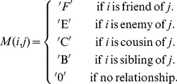 |
(1) |
Consistency within the data was attained by applying logic rules and research hypotheses:
 and
and  are siblings
  at least one says they are the sibling of the other and they have the same surnames.
If
 is sibling to

 is sibling to
  .
.If
 is sibling to
  and
and  is sibling to

 is sibling to
  .
. and
and  are cousins
  at least one says they are the cousin of the other and they have a surname in common.
If
 is cousin to

 is cousin to
  .
.If
 is cousin to
  and
and  is sibling to

 is cousin to
  .
.Friendship is a bilateral relationship.
Enmity is a bilateral relationship.
Rules 1–6 were applied because small children sometimes forgot to mention their kinship ties. Both friendship and enmity relationships were considered reciprocal which is why the analysis was focused on bilateral relationships, that is, the cases in which both students said they were friends ( ‘F’ and
  ‘F’) or enemies (
 ‘E’ and
  ‘E’). Kinship relationships were included as friendship relationships. Therefore, by applying rules 1–8 the adjacency matrices become symmetrical matrices.
Friendship Networks Analysis
Once the symmetrical matrices were generated, a friendship network was created for each studied school and their measurements calculated (all defined in [17]). All three school friendship networks shared the same properties (Table 1):  (average friends per student) was relatively high in all; they were low density networks; they had short path lengths; and a high clustering index. This similarity carried through when they were graphed (Fig. 1B).
Table 1. Friendship network measurements.
| School1 | School2 | School3 | |
| Order | 108 | 226 | 419 |
| Size | 503 | 985 | 1575 |
| <k> | 9.315 | 8.717 | 7.518 |
| Diameter | 5 | 6 | 7 |
| Density | 0.087 | 0.039 | 0.018 |
| Clustering | 0.292 | 0.248 | 0.226 |
| Geodesic | 2.477 | 2.962 | 3.898 |
| Betweenness | 0.014 | 0.009 | 0.007 |
| Closeness | 0.407 | 0.340 | 0.259 |
Figure 1. Friendship network topology.

Figure 1 is a graphic representation of the friendship network topology, each node represents a student and lines between nodes indicate friendship relations. This example with  ,
,  and
and  . A)
. A)  ; B)
; B)  , dashed lines represent introduced shortcuts; and C)
  .
.
When the degree distributions were graphed for each school, we believed that they belonged to Poisson distributions (Fig. 2).
Figure 2. Friendship network degree distributions.

Figure 2 shows degree distribution of friendship networks. Dots: Observed school friendship network degree distributions. Line: Adjusted Poisson( ) distribution (where
  is the maximum likelihood estimator of the goodness of fit tests), with
  ,
,  and
and  for School1, School2 and School3, respectively.
To verify that the friendship networks’ degree distribution originated in a Poisson distribution, we ran goodness-of-fit tests [18]. A Karl-Pearson statistic [19] was used to measure statistical differences between the observed data and the theoretical distribution (i.e. Poisson). For each test,  was the maximum likelihood estimator and in all three cases the p-value was sufficiently significant (Table 2), and therefore evidence exists that the friendship network distributions originated in a Poisson(
 ) distribution; see the adjusted Poisson distributions (Fig. 2).
Table 2.
 test results.
| School1 | School2 | School3 | |
| <k> | 9.315 | 8.717 | 7.518 |
| χ 2 | 16.997 | 20.441 | 24.703 |
| p-value | 0.107 | 0.059 | 0.025 |
 test results, we prove that observed data meet a Poisson(
 ) distribution, where
  is the maximum likelihood estimator.
Given the Poisson distribution of the friendship networks at the three schools, it can be expected that they could be reproduced with the Erdös-Rényi (ER) model [20] because this generates complex networks with a degree distribution given by.
| (2) |
The ER model has two parameters:  is the network order; and
  is the probability that a link exists between any
  and
and  node pair. However, the clustering index will be low because in ER networks the clustering index (
 ) tends to be equal to network density. In the studied system, this means that the model did not reproduce the fact that if
  and
and  have a common friend in a certain student then
  and
and  tend to be friends also.
The Watts-Strogatz (WS) model [21] is known to produce networks with high clustering index values. This model has three parameters:  is the network order;
  is the degree of the initial regular network; and
  is the probability of redirecting each network link. However, the degree of distribution for WS networks, developed in [22], is given by.
 |
(3) |
and defined by  , with
  and
and  . On the one hand, distribution 3 differs significantly from the Poisson distribution in that it tends to centralize in
  . In the present study system, this is equivalent to saying that almost all the students would have
  friends, thus leaving out introvert (few friendship relationships) and extrovert (many friendship relationships) students. On the other hand, distribution 3 tends toward a Poisson distribution when parameter
  , but when this occurs the model tends toward an ER model and, as mentioned previously, the ER model does not reproduce all observed measurements.
Friendship Network Model
Neither the ER nor the WS models completely reproduced the friendship networks at the three studied schools. In response, we decided to develop a model to more accurately represent them. All three friendship networks exhibited spatial confinement caused by the fact that in schools students are grouped by classroom which is where they primarily interact. In other words, a student in a given classroom (e.g.  grade) has lots of friends in his classroom but few in other classrooms. In addition, students also experience a sense of belonging to a social group [23], [24]. These phenomena cause friendship networks to exhibit the atypical characteristic of a Poisson topology coupled with a high clustering index.
Spatial confinement and a sense of belonging are significant phenomena in these networks and were thus considered when designing the proposed model. What we call the School Friendship Network (SFN) encompasses four parameters:  , number of students;
  , number of classrooms in the school;
  , average number of friends per student; and
  , the probability of introducing shortcuts into the network. The goal was for the SFN model to reproduce the degree distribution and measurements observed in the three studied schools.
Spatial Confinement and Sense of Belonging to a Social Group
To reproduce spatial confinement, it was decided to generate  isolated networks
  for
for  , where each
  has the probabilistic construction ER
 representing the friendship relationships within each classroom (Fig. 1A). In this way,
  has
has  students (nodes) and a degree distribution as follows.
| (4) |
where  is the probability of any two students in the same classroom being friends. Given that in the ER networks
  (
( density) and
  (
( clustering index) are met, then from the first property follows
| (5) |
Given that the entire network, called  , is defined by
  , then the degree distribution is also given by distribution 4, and its clustering index, denoted
  , is given by.
| (6) |
Equation 6 indicates that  depends on
  and
and  such that when classrooms are sufficiently large with respect to
  ,
,  will be small. This assumes a problem in model construction. However, group dynamic theory [23] describes two types of groups: primary [25], and secondary [26]. Primary groups are composed of a small number of members with affective and intimately bonded relationships which share interests, values, goals, etc., and each member has a sense of belonging to the group. Secondary groups, in contrast, have a large number of members, which precludes proximity amongst them and any proximity is generally imposed (e.g. by institutional rules). In the relationship between these two group types, primary groups tend to appear within secondary groups. Taking this into account, we considered that relatively small classrooms have primary group characteristics, that is, members have a sense of belonging to the social group where they are spatially confined. If the group is large, however, it will have secondary group characteristics with primary groups forming within it which then interact inside the classroom in which they are spatially confined. We use this to apply a rule that will allow creation of subgroups within classrooms. Of note is that the social phenomenon of primary group formation within large classrooms also occurs at the studied schools, although it is not as evident as spatial confinement. We refer here to the fact that the spatial confinement produced by grouping into classrooms is evident in the adjacency matrices, but grouping within the classrooms produced by sense of belonging to a primary group is only evident in detailed observation of the interaction networks.
Based on the observed clustering indices, we proposed a threshold such that if  , therefore, instead of creating
  networks,
  subnetworks are created within each
  classroom, where
  is given by
| (7) |
By applying this process,  will be within the interval
  and the total network will be
  , with
  for
for  . To create each one of the
  networks, a recursive process was applied which is analogous to that described previously in this subsection.
Adding Shortcuts
The function  = shortcuts
 receives two parameters, where
  is a network composed of isolated subnetworks and
  is the probability of creating shortcuts in
  network. This is done by eliminating each
  link with the probability
  , thus creating a new link between two randomly chosen
  nodes. This process creates a
  network which conserves the same number of nodes and links as
  (Fig. 1B).
Algorithm
The algorithm for the SFN model involves four steps:
Calculate
 , where
  is the number of students per classroom.
-
If
 :
:Calculate
 of Equation 7, where
  is the number of subnetworks for each classroom.
Calculate
 and
and  , where
  is the number of students in each subnetwork (within each classroom) and
  is the probability that any two students in the same subnetwork (within each classroom) will be friends.
For each of
 classrooms: Create
  ER
ER networks.
For each of
 classrooms: Apply the shortcuts
 function, where each
  is the network formed by
  isolated networks.
-
If
 :
:Calculate
 , where
  is the probability that any two students in the same classroom will be friends.
For each of
 classrooms: Create an ER
 network.
Apply the shortcuts
 function, where
  is the network formed by
  isolated networks.
In this way the model defines networks that are an interpolation between totally random isolated networks with a binomial distribution ( ) and a totally random network with a Poisson distribution (
 ) (Fig. 1). Each of the subnetworks (Fig. 1A), as well as the overall network (Fig. 1C), have the same probabilistic construction. Of note is that parameter
  was expressly introduced, and a future research goal is to find a theoretical way of calculating
  .
.
When the SFN model was applied to the data, measurements (Table 3) and distributions (Fig. 3) did not differ from those observed in the studied schools. We ran Kolmogorov-Smirnov tests [18] to verify that the distributions produced by the SFN model did not differ statistically from the observed distribution (i.e. null hypothesis). The resulting p-values (School1  ; School2
  ; School3
  ) indicate that there is enough evidence to confirm that the distributions generated by the SFN model did not differ significantly from the empirical distributions.
Table 3. Friendship network measurements generated with SFN model.
| SFN1 | SFN2 | SFN3 | |
| Order | 108 | 226 | 419 |
| Size | 502.84 | 985.13 | 1574.8 |
| <k> | 9.312 | 8.718 | 7.517 |
| Diameter | 4.684 | 5.913 | 6.918 |
| Density | 0.087 | 0.039 | 0.0180 |
| Clustering | 0.284 | 0.239 | 0.221 |
| Geodesic | 2.550 | 3.211 | 3.832 |
| Betweenness | 0.014 | 0.010 | 0.007 |
| Closeness | 0.395 | 0.315 | 0.261 |
Friendship network measurements generated with the proposed model. SFN1:  ,
,  ,
,  and
and  . SFN2:
  ,
,  ,
,  and
and  . SFN3:
  ,
,  ,
,  and
and  . Each value corresponds to an average over
  independent simulations.
Figure 3. Friendship network degree distribution with SFN model.

Figure 3 shows degree distribution of friendship networks with SFN model. Circles:  ,
,  ,
,  and
and  . Squares:
  ,
,  ,
,  and
and  . Triangles:
  ,
,  ,
,  and
and  . Each point corresponds to an average over
  independent simulations.
Studies do exist of friendship networks in a school environment [2], [27] (e.g. Zachary karate club [28], college football [2]), but these are aimed at developing models to detect communities. The SFN model creates communities to produce a structure similar to the observed networks, with the same approximate measures and distributions.
Enmity Network Analysis
Among the three studied schools, the enmity networks had similar measurements; for example, all three had low  (average enemies per student) values, were low density networks, had short path lengths and a low clustering index value (Table 4). Since the three networks happen to be not connected, the diameter and betweenness are calculated from the principal component, while geodesic was estimated as the reciprocal of closeness. All three networks also had a similar structure when graphed (Fig. 4B). Degree distribution for the three schools (School1, School2, School3) was believed to conform to power law distributions (Fig. 5).
Table 4. Enmity network measurements.
| School1 | School2 | School3 | |
| Order |

|

|
419 |
| Size |

|

|

|
| <k> |

|

|

|
| Diameter |

|

|

|
| Density |

|

|

|
| Clustering |

|

|

|
| Geodesic |

|

|

|
| Betweenness |

|

|

|
| Closeness |

|

|

|
Figure 4. Enmity network topology.

Figure 4 is a graphic representation of the enmity network topology, each node represents a student and lines between nodes indicate enmity relations. This example with  ,
,  and
and  . A)
. A)  ; B)
; B)  , dashed lines represent introduce shortcuts; and C)
  .
.
Figure 5. Enmity network degree distributions.

Figure 5 shows degree distribution of enmity networks. Dots: Observed school enmity network degree distributions. Line: Potential regression model  , with
  ,
,  ;
;  ,
,  and
and  ,
,  for School1, School2 and School3, respectively. Inset: Kolmogorov-Smirnov test, observed data and adjusted power law.
To verify that the enmity networks degree distributions originated in a power law distribution, potential regression tests [29] were done with the model  . This was done without including
  . The
. The  -adjusted was greater than
  in all three cases (Table 5), although this test is inconclusive, only suggesting that the observed data could be distributed under a power law.
Table 5. Potential regression model adjustment and Kolmogorov-Smirnov test results.
| School1 | School2 | School3 | |
| γ |

|

|

|
| C |

|

|

|
| R 2-adjusted |

|

|

|
| α |

|

|

|
| kmin |

|

|

|
| p-value |

|

|

|
Top: Potential regression model adjustment,  -adjusted value show fit greater than
  in all three cases. Bottom: Kolmogorov-Smirnov test results, we prove that observed data meet a distribution in equation 8, where
  is the lowest
  value for which the power distribution hold and
  is the maximum likelihood estimator.
Kolmogorov-Smirnov tests, described in [30], were run to improve validation, adjusting the data to the distributions
| (8) |
where  is the lowest
  value for which the power distribution is met and
  is the maximum likelihood estimator for the observed data; both were estimated as described in [30]. This test uses the
  statistic, which measures the maximum absolute difference of the accumulated distribution functions for the observed data and theoretical distribution. In all three cases, the p-value
 , and therefore evidence exists that the enmity network distribution tails originated in a power law (Table 5). This is visible in the graphics showing the observed data and corresponding adjusted power law for each school (Fig. 5).
Once it was clear that the enmity networks exhibited a distribution with a power law tail, it is to be expected that the Barabási-Albert (BA) model [31] could reproduce them. This model has a distribution given by
| (9) |
where  and
and  . There are two parameters in the BA model:
  is the network order, and
  is the number of links contributed by each node as it enters the network. However, this model produces networks in which all nodes are at least 1 degree and are connected. This means that these networks’ degree distributions differed significantly from those of the studied enmity networks.
Enmity Network Model
Once it was confirmed that the enmity networks were not completely reproduced by the BA model, we decided to develop a model to more accurately represent them. Distributions exist with this form.
| (10) |
where  [30]. Based on the previous tests and the Fig. 5 (graphics inset), we conclude that distribution 10 best represents the observed data. This being the case, the proposed model must contemplate both preferential attachment (to model the power law) and randomness (to model the exponential) when links are introduced into the network. As is to be expected, spatial confinement also occurs in the studied enmity networks, which is why the School Enmity Network (SEN) includes four parameters:
  is number of students;
  is number of classrooms;
  is average number of enemies per student; and
  is the probability of introducing shortcuts into the networks. In contrast to the SFN model, the SEN model generates networks with preferential attachment, applying the rules.
| (11) |
where  is the degree of node
  , that is, a node has a greater probability of being selected when its degree is higher. The SEN
 model algorithm is as follows.
Calculate
 and
and  , where
  is number of students per classroom and
  is number of enmity relationships per classroom.
For each one of
 classrooms: Create a
  network (
 ) with preferential attachment, where
  will have
  nodes and
  links introduced by connecting two of its nodes, one chosen preferentially according to equation 11 and the other chosen randomly (Fig. 4A).
For each link in the
 network (
 ), this is eliminated with probability
  and a new link created between two
  nodes (one chosen preferentially according to equation 11 and the other chosen randomly).
Therefore, the model defines networks which are an interpolation between isolated preferential attachment networks ( ) and a preferential attachment network (
 ) (Fig. 4). As occurred with the SFN model, each of the subnetworks (Fig. 4A) and the overall network (Fig. 4C) had the same probabilistic construction. Measurements were then generated by applying this model to the observed data (Table 6), and degree distributions for these networks graphed (Fig. 6). We ran Kolmogorov-Smirnov tests comparing the SEN model distributions with the observed distributions. The resulting p-values (School1
  , School2
  , School3
  ) indicate that these distributions do not differ significantly from the empirical values.
Table 6. Enmity network measurements generated with SEN model.
| SEN1 | SEN2 | SEN3 | |
| Order |

|

|

|
| Size |

|

|

|
| <k> |

|

|

|
| Diameter |

|

|

|
| Density |

|

|

|
| Clustering |

|

|

|
| Geodesic |

|

|

|
| Betweenness |

|

|

|
| Closeness |

|

|

|
Enmity network measurements generated with the proposed model. SEN1:  ,
,  ,
,  and
and  . SEN2:
  ,
,  ,
,  and
and  . SEN3:
  ,
,  ,
,  and
and  . Each value corresponds to an average over
  independent simulations.
Figure 6. Enmity network degree distribution with SEN model.

Figure 6 shows degree distribution of enmity networks with SEN model. Circles:  ,
,  ,
,  and
and  . Squares:
  ,
,  ,
,  and
and  . Triangles:
  ,
,  ,
,  and
and  . Each point corresponds to an average over
  independent simulations.
Models do exist which are more flexible in response to the introduction of links into the network (e.g. extended BA model [32]). Depending on their parameters, they can generate networks with distribution 10, even though these do not consider the spatial confinement, a characteristic vital to reproducing the structure of the networks we are studying.
Conclusions and Discussion
In the three studied schools, friendship relationships had a Poisson topology while enmity relationships had a power law topology. New models were necessary to accurately reproduce the observed data, both in terms of measurements and degree distributions. Spatial confinement and a sense of belonging to a social group both played important roles since their incorporation allowed studying and understanding the characteristics and phenomena which occur in the studied school networks.
As mentioned in section ‘Methodology’, School1 had one classroom containing two grades ( and
and  ). For study purposes, these groups were treated as separate classrooms because the principle observed in subsection ‘Spatial confinement and sense of belonging to a social group’ was observed here. Despite the spatial confinement in this classroom, the sense of belonging to a primary group was manifested. In response, two subgroups were created, one of
  grade students and the other of
  grade students, with some interactions between them, exactly as if they were two classrooms.
Promising future research areas include theoretical analysis of the network properties produced in these models. Another possible study would be to apply a diffusion process (e.g. disease transmission) to these networks, observe how the disease infects other students and propose ways of preventing propagation. An analysis could also be run of the link(s) between the friendship network and enmity network within the same school. Another interesting area of inquiry is network assortativity classes [33], that is, the tendency observed in social networks in which nodes connect to other nodes with similar properties. This property generally refers to the degree of nodes, but we can also speak of social assortativity (as mentioned previously) in the studied friendship and enmity networks. Assortativity manifests in our model because students mainly relate to students in their own classroom. After analyzing the networks, however, other types of assortativity become evident, such as sex, in which boys have friendships and enmities mainly with boys and girls mainly with girls. In rural schools, assortativity occurs based on kinship in that students have friendships with relatives, although this does not hold for enmity networks.
The proposed models (SFN and SEN) generated complex networks with fractal characteristics. It is highly probable that a study of the friendship and enmity networks between students from different schools in the same location would find that the relationships between schools have the same structure as the relationships observed here between classrooms. In other words, there would be a high number of relationships between students at the same school and few between students from different schools. This pattern could repeat itself in an analysis of relationships between students from different locations, thus forming a fractal structure. If this were the case, the proposed models could be generalized and used to represent the network structure of an entire community, although reaching this point will require further research.
Acknowledgments
The authors thank the administrators and teachers of ‘Silvestre Chi Elementary School’, ‘Rafael Ramírez Castañeda Elementary School’ and ‘Ignacio Zaragoza Elementary School’ in Yucatán, México, for allowing us to carry out part of this study with their students. Thanks also to Arely Paredes-Chi and Karla Atoche-Rodríguez, Environmental Education Ph.D. students at Deakin University, Australia, for their assistance in applying the data collection instruments in the studied schools.
Funding Statement
There were no funders for this research.
References
- 1. Jackson MO, Wolinsky A (1996) A Strategic Model of Social and Economic Networks. J Econ Theory 71: 44–74. [Google Scholar]
- 2. Girvan M, Newman MEJ (2002) Community Structure in Social and Biological Networks. PNAS 99: 7821–7826. [DOI] [PMC free article] [PubMed] [Google Scholar]
- 3. Albert R, Jeong H, Barabási AL (1999) Diameter of the World Wide Web. Nature 401: 130–131. [Google Scholar]
- 4. Lozano S, Arenas A, Sánchez A (2008) Mesoscopic Structure Conditions the Emergence of Cooperation on Social Networks. PLoS ONE 3(4): e1892 doi:10.1371/journal.pone.0001892. [DOI] [PMC free article] [PubMed] [Google Scholar]
- 5. Apicella CL, Marlowe FW, Fowler JH, Christakis NA (2012) Social networks and cooperation in hunter-gatherers. Nature 481: 497–501. [DOI] [PMC free article] [PubMed] [Google Scholar]
- 6. Villas Boas PR, Rodrigues FA, Travieso G, Costa LdaF (2010) Sensitivity of Complex Networks Measurements. J Stat Mech 3: P03009. [Google Scholar]
- 7. Barabási AL, Albert R, Jeong H (1999) Mean-field Theory for Scale-free Random Networks. Physica A 272: 173–187. [Google Scholar]
- 8. Amaral LAN, Scala A, Barthélémy M, Stanley HE (2000) Classes of Small-World Networks. PNAS 97: 11149–11152. [DOI] [PMC free article] [PubMed] [Google Scholar]
- 9. Boccaletti S, Latora V, Moreno Y, Chavez M, Hwang DU (2006) Complex Networks: Structure and Dynamics. Phys Rep 424: 175–308. [Google Scholar]
- 10. Cattuto C, Van den Broeck W, Barrat A, Colizza V, Pinton J-F, et al. (2010) Dynamics of Person-to-Person Interactions from Distributed RFID Sensor Networks. PLoS ONE 5(7): e11596 doi:10.1371/journal.pone.0011596. [DOI] [PMC free article] [PubMed] [Google Scholar]
- 11. Salathé M, Kazandjieva M, Lee JW, Levis P, Feldman MW, et al. (2010) A High-Resolution Human Contact Network for Infectious Disease Transmission. PNAS 107: 22020–22025. [DOI] [PMC free article] [PubMed] [Google Scholar]
- 12. Stehlé J, Voirin N, Barrat A, Cattuto C, Isella L, et al. (2011) High-Resolution Measurements of Face-to-Face Contact Patterns in a Primary School. PLoS ONE 6(8): e23176 doi:10.1371/journal.pone.0023176. [DOI] [PMC free article] [PubMed] [Google Scholar]
- 13. Mednick SC, Christakis NA, Fowler JH (2010) The Spread of Sleep Loss Influences Drug Use in Adolescent Social Networks. PLoS ONE 5(3): e9775 doi:10.1371/journal.pone.0009775. [DOI] [PMC free article] [PubMed] [Google Scholar]
- 14. Onnela JP, Arbesman S, González MC, Barabási AL, Christakis NA (2011) Geographic Constraints on Social Network Groups. PLoS ONE 6(4): e16939 doi:10.1371/journal.pone.0016939. [DOI] [PMC free article] [PubMed] [Google Scholar]
- 15. Hock K, Fefferman NH (2011) Violating Social Norms when Choosing Friends: How Rule-Breakers Affect Social Networks. PLoS ONE 6(10): e26652 doi:10.1371/journal.pone.0026652. [DOI] [PMC free article] [PubMed] [Google Scholar]
- 16.Hartas D (2010) Survey Research in Education. In: Hartas D, editor. Educational Research and Inquiry. Qualitative and Quantitative Approaches. New York: Continuum International Publishing Group. 257–269.
- 17.Vega-Redondo F (2007) Complex Social Networks. Cambridge: Cambridge University Press.
- 18.Thas O (2009) Comparing Distributions. New York: Springer Publishing Company.
- 19. Plackett RL (1983) Karl Pearson and the Chi-Squared Test. Int Stat Rev 51: 59–72. [Google Scholar]
- 20. Erdös P, Rényi A (1960) On the Evolution of Random Graphs. Publ Math Inst Hung Acad Sci 5: 17–61. [Google Scholar]
- 21. Watts DJ, Strogatz SH (1998) Collective Dynamics of ‘Small-World’ Networks. Nature 393: 440–442. [DOI] [PubMed] [Google Scholar]
- 22. Barrat A, Weigt M (2000) On the Properties of Small-World Network Models. Eur Phys J B 13: 547–560. [Google Scholar]
- 23.Hogg MA, Abrams D (1998) Social Identifications: a Social Psychology of Intergroup Relations and Group Processes. New York: Routledge.
- 24.Capozza D, Brown R (2000) Social Identity Processes: Trends in Theory and Research. London: SAGE Publications.
- 25.Cooley CH (2005) Social Organization: a Study of the Larger Mind. Introduction by Philip Rief. New Jersey: Transaction Publishers.
- 26.Olmsted MS (1963) The Small Group. New York: Random House.
- 27.Balakrishnan H, Deo N (2006) Discovering Communities in Complex Networks. Proceedings of the 44th Annual Southeast Regional Conference. New York: Association for Computing Machinery. 280–285.
- 28. Zachary WW (1977) An Information Flow Model for Conflict and Fission in Small Groups. J Anthropol Res 33: 452–473. [Google Scholar]
- 29.Casella G, Berger RL (2002) Statistical Inference 2ed. California: Duxbury.
- 30. Clauset A, Rohilla C, Newman MEJ (2009) Power-Law Distributions in Empirical Data. SIAM Review 51: 661–703. [Google Scholar]
- 31. Barabási AL, Albert R (1999) Emergence of Scaling in Random Networks. Science 286: 509–512. [DOI] [PubMed] [Google Scholar]
- 32. Albert R, Barabási AL (2000) Topology of Evolving Networks: Local Events and Universality. Phys Rev Lett 85: 5234–5237. [DOI] [PubMed] [Google Scholar]
- 33. Newman MEJ (2002) Assortative Mixing in Networks. Phys Rev Lett 89: 208701. [DOI] [PubMed] [Google Scholar]