Context-Sensitive Markov Models for Peptide Scoring and Identification from Tandem Mass Spectrometry

Abstract

Peptide and protein identification via tandem mass spectrometry (MS/MS) lies at the heart of proteomic characterization of biological samples. Several algorithms are able to search, score, and assign peptides to large MS/MS datasets. Most popular methods, however, underutilize the intensity information available in the tandem mass spectrum due to the complex nature of the peptide fragmentation process, thus contributing to loss of potential identifications. We present a novel probabilistic scoring algorithm called Context-Sensitive Peptide Identification (CSPI) based on highly flexible Input-Output Hidden Markov Models (IO-HMM) that capture the influence of peptide physicochemical properties on their observed MS/MS spectra. We use several local and global properties of peptides and their fragment ions from literature. Comparison with two popular algorithms, Crux (re-implementation of SEQUEST) and X!Tandem, on multiple datasets of varying complexity, shows that peptide identification scores from our models are able to achieve greater discrimination between true and false peptides, identifying up to ∼25% more peptides at a False Discovery Rate (FDR) of 1%. We evaluated two alternative normalization schemes for fragment ion-intensities, a global rank-based and a local window-based. Our results indicate the importance of appropriate normalization methods for learning superior models. Further, combining our scores with Crux using a state-of-the-art procedure, Percolator, we demonstrate the utility of using scoring features from intensity-based models, identifying ∼4-8 % additional identifications over Percolator at 1% FDR. IO-HMMs offer a scalable and flexible framework with several modeling choices to learn complex patterns embedded in MS/MS data.

Introduction

Rapid advances in the field of proteomics are elucidating fundamental biomolecular processes such as protein expression and interactions, post-translational modifications, and their role as biomarkers of clinical conditions in diseases (Vitek, 2009). Tandem Mass Spectrometry (MS/MS) coupled with Liquid Chromatography is one such key methodology facilitating large-scale identification and characterization of proteins in complex samples such as plasma, urine, and blood (Aebersold et al., 2001; Nesvizhskii, 2007). Routine MS/MS experiments yield large datasets of mass-spectra and require confident identification of peptides that generated them. A typical approach to achieve this goal is called Database Searching, and proceeds via scoring candidate peptides (obtained from a protein sequence database) against experimental spectra for possibility of a match (Nesvizhskii et al., 2007; Steen et al., 2004).

A critical step in scoring involves theoretical modeling of peptide fragmentation. The scorer then compares the theoretical with experimental spectra to compute agreement. Several scoring algorithms, some heuristic while others probabilistic, have been developed, some widely used being SEQUEST (Eng et al., 1994), Mascot (Perkins et al., 1999), X!Tandem (Craig et al., 2004), MyriMatch (Tabb et al., 2007), and OMSSA (Geer et al., 2004). These algorithms are routinely applied to complex proteomic investigations. However, they rely on oversimplified theoretical fragmentation models and heuristics that either completely ignore or underutilize the intensity dimension of MS/MS spectra. In large-scale experiments, less than 30% spectra are confidently assigned with peptides, and inadequacies of scoring algorithms is a key contributing factor, among others (Marcotte, 2007).

Our overall research goal is to incorporate the influence of peptide physicochemical properties on fragmentation, into the process of their scoring. Recent studies have shown that peptide fragmentation is reproducible under similar experimental conditions, and hence theoretically predictable (Hubbard et al., 2010; Paizs et al., 2005). A qualitative theory called the “Mobile Proton Theory” identifies that under low-energy conditions (the usual situation), peptide fragmentation strongly depends on the “mobility” of the added charge along the peptide backbone. Mobility, in turn, depends on the peptide primary structure, charge state, and positions of basic residues on the peptide chain (Paizs et al., 2005; Tabb et al., 2004; Wysocki et al., 2000). Effects of several amino acids on fragmentation behavior have also been investigated and clearly establish the link between the peptide primary structure and its fragmentation efficiency (Breci et al., 2003; Tabb et al., 2004; Tsaprailis et al., 2004; Vaisar et al., 1996). These developments, along with accessibility to large repositories of complex MS/MS datasets, have encouraged the use of machine learning algorithms for learning fragmentation patterns (Craig et al., 2004; Desiere et al., 2006; Martens et al., 2005).

Elias et al. (2004) used probabilistic decision trees (Jensen et al., 2007) to model intensity distributions of peptide fragments from a large set of peptide properties. Zhou et al. (2008) used similar properties with a Bayesian artificial neural network (Bishop, 1996) for predicting intensities of the commonly observed b- and y-ions. Although a significant advance, these algorithms assume independence of fragments and ignore any correlations that might exist in series of observed ion intensities. Klammer et al. (2008) used dynamic bayesian networks (Murphy, 2002) to model the intensities of different fragment ion-types, individually as well as in pairs, and utilized a smaller set of physicochemical properties. Scores from their models were combined using the support vector machine (SVM) (Cortes et al., 1995; Vapnik 1998) algorithm to discriminate true from false peptide identifications. Khatun et al. (2008) used a Hidden Markov Model (HMM) (Rabiner, 1989) to learn intensity dependence on ion-type and their mass distributions, as well as on flanking amino acids

In this article, we present a novel scoring algorithm called Context-Sensitive Peptide Identification (CSPI) that builds upon these recent fragmentation models and principles underlying peptide fragmentation. Our methods are based on Input-Output Hidden Markov Models (IO-HMM) (Bengio et al., 1995; Bengio et al., 2001), which are used to stochastically model data that contain pairs of sequences, called ‘input’ and ‘output’. In the case of peptide identification, ‘input’ refers to a representation of the peptide sequence, while ‘output’ refers to a representation of the MS/MS spectrum intensities. The modular architecture of IO-HMM can represent complex probability distributions using varied functional forms. Their sequential nature captures dependencies between observed fragment-ion intensity series, facilitating learning and computing the desired probability, P(spectrum | peptide).

To illustrate these capabilities, we include several features in our models that are known to influence peptide fragmentation. We also evaluate two intensity normalization schemes (output representation). Using this framework, we show significant improvement in peptide identification accuracies as compared with two popularly used algorithms: Crux (Park et al., 2008) and X!Tandem (Craig et al., 2004). In addition, we combine the individual heuristic scores using a recent state-of-the-art score combination procedure called Percolator (Kall et al., 2007) and demonstrate the utility of intensity-based models. Percolator was chosen due to its good performance characteristics and ease of implementation. To the best of our knowledge, this is the first study that develops and tests an IO-HMM-based modeling framework to score peptide-spectrum matches (PSMs). Being highly flexible and scalable, it is easy to extend resulting models using additional features/context, thus making them attractive to explore further.

Materials and Methods

CSPI model structure and parameterization

IO-HMMs are an extension of the classic Hidden Markov Models (HMM) and are used to model sequence pairs rather than individual sequences (Fig. 1). In the discussion that follows, we denote a generic input sequence as and an output sequence as , where ‘t’ refers to the location within the sequences being modeled, while ‘T’ is the total length of the sequence. We use the same length ‘T’ for all sequences for notational convenience.

FIG. 1.

(A) Classical Hidden Markov Model; (B) Input-Output Hidden Markov Model.

The model represents the conditional probability distribution , where ‘Θ’ are the model parameters. Similar to HMM, an intermediate hidden layer facilitates modeling sequential dependencies. However, the additional conditioning on the input layer makes the transition and/or emission probability distributions potentially nonstationary in location. This means that, unlike HMM, instead of a transition matrix (or emission vector) of probabilities that remains fixed throughout the hidden layer, we now have a probabilistic function that takes the context (input features x_t) available at the specific location ‘t’ under consideration, thus facilitating dynamic mapping of input-to-output sequences. Both x_t and y_t can be univariate or multivariate, discrete or continuous, whereas the hidden states, q_t, are typically discrete. Additionally, the input sequence can be constructed with arbitrary features (from the domain) that may or may not overlap in location, allowing rich contextual information at local (specific location), as well as global (sequence) level to be incorporated in the sequence mapping tasks. The goal, then, is to learn the sequential dependencies between the input and the output.

Input Layer ()

Our input layer is a sequential representation of the peptide sequence being evaluated. Each amide-bond position in the peptide sequence (from N- to C-terminus) is represented as a feature vector that forms the ‘input’ x_t at the corresponding location, and represents the global (peptide- or fragment-level) and local (fragmentation site-level) context influencing observed fragmentation. For example, a peptide of length 10 has 9 amide bond positions and is represented in the input layer as a sequence of 9 feature vectors, each being of same length as the number of features used.

The features used in the model are described in Table 1. The “Mob” feature uses an accepted definition of mobility [ChargeState – Number of Arg – 0.5*(Number of His+Number of Lys)] (Huang et al., 2008). We grouped the mobility values into four bins as shown in the table. Similarly, ‘length’ feature was grouped into three categories: short (<13), medium (between 13 and 23), and long (>=23), binned roughly at 25^th and 75^th percentiles of peptide lengths in the training dataset.

Table 1.

Contextual Features Used in the IO-HMM Input Layer

Feature	Type (Length)	Description	Influence
NAA	Binary (19)	Flanking N-terminal Amino acid (Considering Pro as baseline; 1 binary feature for remaining 19 possible)	Local
CAA	Binary (19)	Same as NAA	Local
FracMz	Numeric (1)	Fractional mass-to-charge (m/z) of fragment relative to the m/z of the parent peptide; Range: (0,1)	Local
Mob	Binary (3)	Mobility value of the peptide (<= 0: baseline; one binary feature for 0.5, 1, >1)	Global
CTerm=R?	Binary (1)	Is the C-terminus of peptide Arg?	Global
K/H in b-fragment	Binary (1)	Is there a Lys or His in the b-fragment (other than NAA/CAA)	Fragment
R in b-fragment	Binary (1)	Is there an Arg in the b-fragment (other than NAA/CAA)?	Fragment
Length	Binary (2)	Length of the peptide, discretized into 3 bins (length<13: baseline; one binary feature each for 13<= len<23 and 23<= len)	Global
Total	47

Output Layer ()

The output layer consists of the sequence of observed intensities of the most predominant fragment ions, b- and y-ions, of the peptide under low energy Collision-Induced Dissociation (CID). Since b- and y-ions follow different intensity distributions, we learn separate IO-HMM models for each, and call them IO-HMM_b and IO-HMM_y, using b- and y-ion intensities as output layer, respectively. The same input features are used in both models. The directionality used in the b-ion models is from N-terminus to C-terminus, while that for y-ion models is from C-terminus to N-terminus. In order to handle wide variation in the observed fragment intensities, instead of using raw values, we subject the spectra to several pre-processing steps before training or testing the models (see section PSM Properties, Spectrum Pre-Processing). Finally, a normalized intensity value is used for each observed fragment at each fragmentation site.

Normalization

We have evaluated two different normalization schemes, which we call “Rank-norm” and “Window-norm”.

For ‘Rank-norm’ scheme (after spectrum pre-processing), the peaks of the spectrum are assigned ranks, which are then normalized to range [0.001, 0.999], 0.001 being the highest intensity and 0.999 being the lowest. This normalization range was chosen instead of [0, 1] to avoid difficulties in parameter estimation for the emission distributions used for rank-norm scheme (see Emission functions, below). Such rank-based normalization has been used in recent studies in order to reduce variation, and makes intensities comparable across spectra (Klammer et al., 2008; Wan et al., 2006). Fragment ions that are not observed in the experimental spectrum are represented as “Null” in the output layer.

For “Window-norm” scheme (after spectrum pre-processing), the output/emission value used is the log of the fraction of intensity explained by the fragment within±75 Da window around its m/z value, the rationale being that the fragments from the true peptide should explain more abundant peaks than those from false peptides. Again, if a fragment is not observed the observation at that location is designated as “Null”.

Parameter representation

IO-HMM, in its most general form, contains two kinds of probabilistic dependencies: a) emission or observation probabilities P(y_t | q_t, x_t), and b) hidden-state transition probabilities P(q_t | q_t-1, x_t); these can be represented with arbitrary probabilistic functions as:

(1)

where f and g are any linear or non-linear functions with valid probabilistic outputs. The parameters Θ of the model comprise the parameters of these emission and transition functions.

Emission functions

In our model, emission functions are represented as simple distributions, conditioned only on the hidden state value (q_t), [i.e., P(y_t | q_t, x_t)=P(y_t | q_t)]. We have used an IO-HMM with four hidden-state values. One is reserved for “Null” emission (i.e., when the fragment is not observed), and has emission probability of 1. The other three values correspond to observed fragments with continuous emission distributions. These can be thought of as states producing “Low”, “Medium”, and “High” intensity observations (on average, determined by the “mean” of the emission distribution used). For rank-norm scheme, we have used Exponential emission distribution for b/y-ions from true peptides and Beta distribution for those from false/random peptides. For window-norm scheme, we have used Gaussian emission distribution for both b/y-ions and from true and false peptides. The distribution of observed intensities of b- and y-ions from validated PSMs was used as a guide for these choices (see Results).

Transition functions

IO-HMM model structure results in one transition function for each hidden-state value. Given the hidden-state value q_t-1=q (t>1) and the context (input x_t), the corresponding function provides the probability distribution over hidden-state values at current location t, [i.e., P(q_t | q_t-1=q, x_t)]. The output of this function changes as the input x_t varies along the peptide sequence. Additionally, there is an initial-state function for computing the distribution over hidden-state values at the start of the sequence [i.e., P(q_t=1 | x_t=1)]. We model all these distributions using logistic functions (see Supplementary Methods, section 1; supplementary data are available online at www.liebertonline.com/omi).

The initial-state and transition functions together predict the hidden state transition probabilities along the peptide sequence. Based on the sequence (context), some state transitions will be more likely than others. IO-HMM models compute probabilities over all such possible state transitions over the entire peptide chain, in order to compute the contribution to the overall score (see Supplementary Methods, section 3).

IO-HMM training

The structure of IO-HMM model is fixed a priori, in terms of input–output representation and number of hidden states. Training consists of estimating the parameters of the model structure from a training dataset which comprises of a set of input-output sequence pairs , where N is the size of the training dataset. These are derived from high-confidence and validated PSMs, with representations as described above. Parameter estimation of IO-HMM is done using the “Maximum-Likelihood” approach. Due to presence of hidden variables () and absence of a closed-form solution, this is achieved using the iterative numerical optimization method called “Generalized Expectation Maximization” (GEM) (Bengio et al., 1995; Dempster A, 1977) (see Supplementary Methods, section 2). Computational complexity of training our models is given by O((s²+p)*L) for each iteration of the EM algorithm, where ‘s' is the number of hidden states, ‘p’ is the number of parameters in the model, and ‘L’ is the sum of lengths of all the input (or output) sequences in the training dataset (Bengio et al., 1995).

IO-HMM inference

Trained IO-HMM models are used to score and rank candidate peptides obtained via Database Search for each spectrum. Inference involves evaluating the joint probability of observing the spectrum (a particular fragment ion series, b- or y-) given the peptide and the model (learned parameters) [i.e., ]. This is done using the ‘Forward Procedure’, which follows similar mechanics as in HMM (Bengio et al., 1995) (see Supplementary Methods, section 3). In order to discriminate between true and false peptide identifications, we learn two different models, one for true PSMs and one for random/false PSMs. In each random PSM, the peptide sequence (input) used is a random/false sequence of (nearly) same mass as the true peptide. We call these models the True and the Null models, with parameters Θ^True and Θ^Null, respectively. The score for a candidate PSM then is computed as the log of likelihood ratio of the spectrum conditioned on the input peptide, from the true and null models:

(2)

Scores from b- and y-ion models are computed in similar fashion, by replacing the output sequence with the normalized intensities of appropriate fragment ion series, b or y. We report the peptide identification performance of three PSM scores: (i) CSPI_Score^b (from IO-HMM_b), (ii) CSPI_Score^y (from IO-HMM_y), and (iii) composite CSPI_Score^byAdded (=CSPI_Score^b+CSPI_Score^y). Further, in order to handle large MS/MS datasets efficiently, we used our recently proposed simple parallelization scheme for the database searching workflow (Grover et al., 2012) (also see Supplementary Methods, section 5).

Datasets

We have evaluated the performance of IO-HMM models on four public datasets of different sizes, complexity and nature, as briefly summarized in Table 2. Details of their experimental protocol can be found in the respective references.

Table 2.

Characteristics of MS/MS Datasets Used for Comparing Algorithms

#	Name	Usage	Size	Instr	Validation	Source
1	SO-DR	Train	13, 249	LCQ+LTQ	FT-ICR	Shewanella Oneidensis, Deinococcus radiodurans (Huang et al., 2008)
2	18Mix1_LCQ	Test	19, 822	LCQ	FDR	Standard 18 protein mix (Mix1) (Klimek et al., 2008)
3	18Mix1_LTQ	Test	53, 507	LTQ	FDR	Standard 18 protein mix (Mix1) (Klimek et al., 2008)
4	Yeast_LTQ	Test	34, 499	LTQ	FDR	Yeast whole cell lysate (Kall et al., 2007)

Since our models contain many tunable parameters, a large training dataset is required to avoid overfitting. In the absence of such large, expert-validated ‘gold-standard’ identifications, a common strategy is to use a set of high-confidence identifications. Dataset 1 (SO-DR) contains high-scoring identifications made initially using the SEQUEST algorithm, and further validated via accurate mass detection at the same retention time by FT-ICR (Marshall et al., 1998) and under identical chromatographic conditions. All identifications that could not be validated were removed from the dataset. As a consequence, a large fraction of these identifications are expected to be correct and hence form a good training dataset for our models. Roughly two-thirds of this data came from an LTQ and remainder from an LCQ instrument. For the current study, all our models were trained using the SO-DR dataset. While SO-DR consisted of only validated high-confidence PSMs, other datasets (18Mix1_LCQ, 18Mix1_LTQ, Yeast_LTQ) are large collections of MS/MS spectra and represent a real-world scenario where the goal is to assign peptides to the spectra and assess significance of the matches.

PSM properties, Spectrum pre-processing

In this work, we have restricted our analysis to a constrained but significant set of peptides. First, only tryptic peptides with both ends adhering to trypsin cleavage specificity are used for all evaluations. Considering imperfect efficiency of trypsin digestion, we also allow up to three internal Lys/Arg residues in peptides where trypsin misses to cleave. Second, we focus on precursor charge state +2 since these peptides fragment well while generating relatively less complex spectra than higher charge states. This class also constitutes the majority for Electospray Ionization (Wilm, 2011), which is widely used for ionizing peptides. Finally, under low-energy collision-induced dissociation (CID), peptides largely fragment at amide bonds along the peptide backbone, (most commonly) yielding singly charged N-terminal fragments (b-ions) and/or a singly charged C-terminal fragments (y-ions); we focus only on these ions. These search parameters were kept the same to the extent possible for all algorithms compared in this work.

As part of building IO-HMM models, we also perform certain pre-processing steps on the MS/MS spectra before they are used either for learning model parameters or searched against databases for candidate peptides. This is crucial so as to make spectra more comparable across each other as well as across multiple datasets, and includes the following steps (in order of operation): a) Remove the peak corresponding to the precursor as this can be very intense and thus overshadow many other shorter peaks; b) Square-root transform all peaks in order to reduce the influence of very intense peaks; c) Normalize all the peaks so that the intensity of the tallest (base) peak is 100, while all other peaks are scaled accordingly; d) Filter noise peaks, where noise threshold is user-defined (default is set to 0.025, i.e., 2.5% or lesser of the base peak); e) Remove the peaks below the low-mass cut-off region (default threshold used is 0.3 times the m/z value of the precursor; ion-trap instruments typically do not retain peaks in this region and filtering reduces the chance of modeling noise); f) finally, select 200 most intense peaks (at max) of those that remain.

The choice of low-mass cut-off is based solely on the properties of the ion-trap instruments that have been established and is commonly used in the literature (Li et al., 2011). As far as noise is concerned, there is no commonly accepted threshold. Our goal was to avoid too stringent a cut-off and at the same time avoid extremely low intensity noisy peaks. This is also the rationale behind choosing the 200 most intense peaks, as is also done in the SEQUEST/Crux algorithm by default. Although these choices have no effect on the complexity (time or space) of the models, they will likely affect the learned parameter values from training the CSPI models. For the purpose of this research, due to computationally intensive nature of training, sensitivity of parameters to different pre-processing choices was not performed.

Database search, performance evaluation

We have compared IO-HMM models with two widely used programs: Crux (version 1.33) (Park et al., 2008) which is a re-implementation of the original SEQUEST algorithm, and X!Tandem (version CYCLONE 2010.12.01.1), which is another popular open-source peptide identification algorithm.

We evaluated MS/MS spectra using the same search parameters to the extent possible, for all algorithms. Candidate sequences were searched using constraints as described above, with a fixed carbamidomethylation modification applied on cysteine residues. We used precursor tolerance of±3.0 Da and fragment tolerance of±0.5 Da. Since IO-HMM models are computationally expensive we applied a simple filter, which picks only top 500 unique candidates for each spectrum, based on their number of theoretical fragments observed in the experimental spectrum. Only these shortlisted peptides are scored using IO-HMM.

For computing and controlling False Discovery Rates (FDR), we use the simple target-decoy strategy described in Kall et al., (2008). Briefly, after performing separate target and decoy searches, FDR at a score threshold, t, is approximated as:

(3)

where n_t(d)=# top - ranked target (decoy) peptides with score≥t

N_t(d)=total number of targets (decoys)

π₀=estimated proportion of target PSMs that are incorrect (fixed at 0.9 as described in Refs. 28 and 33)

Q-values are then computed for each individual PSM as the minimum FDR at which the PSM is called significant. These statistics were computed for Crux, X!Tandem, and IO-HMM using their primary search scores XCorr, Hyperscore, and CSPI_Score^b (or CSPI_Score^y or the composite score CSPI_Score^byAdded), respectively.

Since SO-DR dataset was obtained from Shewanella Onedensis (SO) and Deinococcus radiodurans (DR), the target database used for these spectra was the concatenated protein FASTA sequences for SO and DR (∼7000 proteins). Datasets 18Mix1_LCQ and 18Mix1_LTQ were obtained from controlled mixture of 18 proteins. Hence the target for these spectra was the corresponding set of protein FASTA sequences appended with common contaminant proteins (http://www.thegpm.org/crap/index.html). Likewise, for the Yeast_LTQ dataset, the target used was Yeast FASTA sequences appended with common contaminants (∼6, 500 proteins). Q-values for SO-DR were estimated using two different decoys: reversed SO/DR FASTA and a much larger reversed Human FASTA (∼90,000 proteins; IPI v.74-3, http://www.ebi.ac.uk/IPI). Using a large decoy provides a more rigorous test of performance due to much larger number of candidates being evaluated for each spectrum. For all other test datasets we used reversed Human FASTA appended with corresponding reversed target database as the decoy.

Score combination

The FDR procedure described above can be used to compare performance of different scoring heuristics. However, individual scores are far from perfect and vary a lot from one spectrum to another depending upon PSM properties (such as the spectrum quality, noise-level, the peptide's propensity to fragment and charge-state). Several potentially true PSMs fall in the region where the individual score distribution overlaps with that from false PSMs. One definitive way to improve identification accuracies is to combine several heuristic measures of PSM match-quality, which are also reported alongside with the primary database search score, or by combining the scores from multiple different algorithms. Often such combination provides additional complementary information that can significantly boost performance (Kall et al., 2007; Keller et al., 2002; Searle et al., 2008).

A recent strategy described in the literature is the semi-supervised learning algorithm, Percolator (Kall et al., 2007), which uses a target-decoy approach together with Support Vector Machine (SVM) classifier to combine heuristic scores, learning new parameters for each new dataset. The procedure iterates over the following steps until convergence: a) Identify a set of high-confidence target PSMs to use as positive training data; b) using decoy PSMs as negative training data, train an SVM classifier; c) score the entire set of target PSMs using the trained SVM. The iterations are initialized using high-confidence targets based on SEQUEST cross-correlation score, while subsequent iterations use SVM-based discriminant score. Confidence is measured using q-value (as described earlier) based on these scores. The procedure converges when no new targets are identified at high confidence.

We follow a similar, albeit simplified, strategy as in Percolator with the following two differences: a) we use Logistic Regression classifier instead of SVM, and use the posterior probability of target PSMs from the model as the composite score from which FDR and q-values are computed, and b) we do not learn a cost-matrix for errors in classification. Due to these differences, our implementation, which we call “LogitPercolator” for the remainder of this article, can be considered as the baseline. The procedure provides appropriate weighted combination of CSPI_Score^b and CSPI_Score^y scores, along with other heuristics.

Further details of all the methods can be found in Grover (2015) and in Supplementary Methods.

Results

Normalized intensity distributions

Figures 2 and 3 show the distribution of rank-norm and window-norm intensities for the observed b/y-ions in SO-DR (training) dataset. The upper panel shows the distributions for fragments from true peptides, while the lower panel shows the same for random/false peptides.

FIG. 2.

Distribution of observed rank-normalized intensities of b- and y-ions from True and False/Random PSMs, for SO-DR training dataset. True PSMs consisted of pairs of validated peptide-spectrum matches as reported in the SO-DR dataset. False PSMs were generated from the same spectra by performing database search using reversed SO-DR FASTA database, and randomly selecting one peptide from top 500 candidates based on fraction of total spectrum intensity explained by the candidates.

FIG. 3.

Distribution of observed window-normalized intensities of b- and y-ions from True and False/Random PSMs, for SO-DR training dataset. True and False PSMs used are the same as for Figure 2.

As expected, a larger fraction of the true b/y-ions appear at lower (or higher) intensity values for rank-norm (or window-norm) schemes as compared to false b/y-ions. The separation is greater for y-ions than for b-ions, which is also expected for ion-trap data, which result in more abundant and stable y-ions. The shapes of these distributions guided our choice of emission/output distributions in the IO-HMM models for the two normalization schemes used (as described earlier).

Cross-validation experiment (SO-DR training dataset)

Cross-validation is a commonly used re-sampling strategy, based on splitting the training dataset, to estimate the average performance of statistical models on unobserved data. We performed five-fold cross-validation (5-CFV) on SO-DR dataset by splitting it into five equal parts. Of these, four parts are used for training IO-HMMs while the remaining one-fifth samples are used for testing. The process is repeated five times so that each part becomes the test set once. X!Tandem and Crux do not involve any training, but each time they are evaluated on the same set of one-fifth samples as IO-HMMs to facilitate performance comparison. Database search is performed on each of these test sets as described above. For IO-HMM three scoring schemes were used for computing q-values: (i) CSPI_Score^b, (ii) CSPI_Score^y, and (iii) CSPI_Score^byAdded. For X!Tandem and Crux, their respective primary scores, Hyperscore and XCorr, were used for computing q-values.

Based on the size of the training dataset, each test set consisted of 2649 MS/MS spectra. After performing database search on these and controlling the FDR at q-value<= 1%, we computed the percentage of the (assumed known) correct peptide identifications, retrieved correctly by each scoring heuristic. Here, ‘correctness' refers to the case that the peptide sequence identified is the same as the original high-confidence assignment provided in the dataset. For example, if in a test set ‘n’ is the actual number of correct identifications among all those ‘estimated as correct’ at 1% q-value, the reported performance is computed as n/2649. Table 3 reports this performance averaged over 10 test sets obtained by executing 5-CFV twice (2×5-CFV) on the SO-DR dataset.

Table 3.

Cross-Validation Experiment on SO-DR Dataset Reporting % of (Assumed Known) Correct Identifications, Correctly Retrieved by Respective Scoring Heuristic; All Values are Averaged over 2-times 5-fold Cross-Validation (2649 test MS/MS spectra per fold; q-value=0.01)

	Decoy 1 (Reversed SO-DR)		Decoy 2 (Reversed Human)
Algorithm	Rank-norm	Window-norm	Rank-norm	Window-norm
CSPI_Scoreb	26.8%	39.4%	17.7%	26.6%
CSPI_Scorey	71.0%	75.4%	62.8%	66.5%
CSPI_ScorebyAdded	74.4%	81.6%	64.7%	72.8%
Crux	77.2%		62.0%
X!Tandem	71.7%		63.2%

We observe that over both normalization schemes and decoys, byAdded models perform better than y-ion models, which in turn perform better than b-ion models (p<0.001 from one-sided two-sample paired Wilcoxon signed-rank test). Also, within each group (b-, y- or byAdded models) window-norm scheme outperforms rank-norm (p<0.001), providing a significant boost in the number of correct identifications.

Individually, b-ion models perform unfavorably as compared to both Crux and X!Tandem for both normalization schemes and decoys (p<0.001). On the other hand, y-ion models perform much more favorably (better than X!Tandem for window-norm/decoy-1/2, p<0.001; better than Crux for window-norm/decoy-2, p<0.001; worse than Crux for rank-norm/decoy-1, p<0.001; worse than Crux for window-norm/decoy-1, p<0.05; no significant difference in remaining cases). The composite byAdded models perform the best, particularly for window-norm scheme (better than both Crux and XTandem for window-norm/decoy-1/2, p<0.001; better than Crux and X!Tandem for rank-norm/decoy-2 and rank-norm/decoy-1, respectively, p<0.005; worse than Crux for rank-norm/decoy-1, p<0.01; no significant difference from XTandem for rank-norm/decoy-2). It is worth noting that the commercial version of Crux (i.e., SEQUEST) was used to originally identify the peptides in this dataset, and only validated high-confidence PSMs were retained. Despite this bias in favor of Crux, our IO-HMM models show superior performance, particularly for the composite score and window-norm scheme.

Independent test dataset validation

A more reliable evaluation is to train and test on completely different datasets. In Figure 4, we report q-value plots for different algorithms compared when the IO-HMM models were trained on SO-DR dataset while tested on the 18Mix1_LCQ and 18Mix1_LTQ datasets.

FIG. 4.

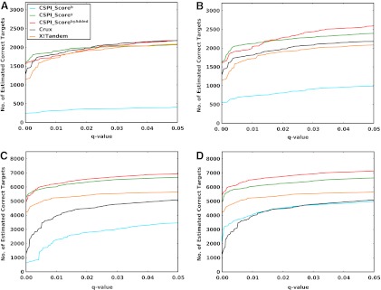
FDR curves; Train on SO-DR dataset, test on: (A) 18Mix1_LCQ, Rank-normalization; (B) 18Mix1_LCQ, Window-normalization; (C) 18Mix1_LTQ, Rank-normalization; (D) 18Mix1_LTQ, Window-normalization. Q-value is a measure of FDR. Different scoring measures are compared using target-decoy strategy, and higher number of estimated correct targets is considered better.

Here we see similar trends in terms of relative performance of heuristics based on IO-HMM models. Specifically, the composite score CSPI_Score^byAdded (red) outperforms the individual b- or y-ion models (blue and green, respectively) for both normalization schemes except for 18Mix1_LCQ dataset (upper panel) for which y-ion models perform better at lower q-values. Comparing rank-norm (left panel) with window-norm (right-panel) scheme, we see a significant performance improvement in both b- and y-ion models, and therefore the composite byAdded score, except for y-ions (green) for 18Mix1_LTQ (lower panel) which perform comparably for both normalizations. We note that the contribution of b-ion models to the composite score appears to be limited and needs further investigation and fine-tuning. Both IO-HMM_y and IOHMM_byAdded models outperform Crux and X!Tandem by a wide margin over an acceptable range of q-values (<0.05) for window-norm scheme on both datasets, and for rank-norm scheme on 18Mix1_LTQ dataset. Specifically, at q-value=0.01, IO-HMM models can achieve over ∼25% improvement in the number of estimated correct peptide identifications.

In order to test the generalization of results from controlled protein mixture to a real-world dataset, we evaluate performance on an additional dataset, Yeast_LTQ. This dataset was generated from yeast whole-cell lysate and consists of a set of ∼35K spectra. We trained IO-HMM models on SO-DR dataset, and Figure 5 shows the corresponding q-value plots. Again, we see a significant performance boost in byAdded models using window-norm scheme, with contribution from improvement in both b- and y-ion models as compared with rank-norm scheme. Additionally, for the window-norm scheme y-ion and byAdded models significantly outperform both X!Tandem and Crux, with ∼11% and 22% more estimated correct identifications (than X!Tandem, which does better than Crux in this case) at q-value=0.01, respectively. All of the above results were generated from CSPI models with four hidden states that achieve a good balance between model performance and complexity. Supplementary Methods (section 4) provides further evidence supporting this choice, by comparing results with three and five hidden states for the Yeast_LTQ dataset.

FIG. 5.

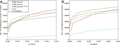
FDR curves; Train on SO-DR dataset, test on: (A) Yeast_LTQ, Rank-normalization; (B) Yeast_LTQ, Window-normalization. Interpretation is same as for Figure 4.

Score combination

As described earlier, multiple heuristics, either from the same or different search algorithms, can be combined to achieve greater performance. In this experiment, we have evaluated the benefit achieved by adding our intensity-based scores from IOHMM on top of other heuristics and scores. Top-ranking PSMs (both targets and decoys) were first extracted from Crux results' files using in-house python scripts, after which IOHMM models trained on SO-DR dataset were applied to them. For this experiment, random decoy peptide sequences generated by Crux were used instead of those from reversed human FASTA. Different sets of features were combined using LogitPercolator and also compared with original Percolator applied on Crux results. Since, from previous results, it is clear that window-norm is superior to rank-norm scheme, this section evaluates LogitPercolator only on window-norm scheme.

Figure 6 shows the q-value plots for various combinations of features, from 18Mix1_LCQ, 18Mix1_LTQ, and Yeast_LTQ datasets. As expected, a dramatic increase in performance is observed as compared with results in the previous section where a single scoring heuristic was used (up to ∼63 % extra estimated correct identifications at q-value=0.01 than the best performing individual heuristic). Without IOHMM scores, comparable performance was achieved for 18Mix1_LTQ and Yeast_LTQ datasets by our baseline LogitPercolator(Crux+) compared to that of the original Percolator, which provides confidence in our comparison and interpretation. Further addition of IOHMM-based heuristics provides upto ∼4%–8% additional estimated number of correct identifications than without them, at q-value=0.01. However we note that ‘delta_IOHMM’ scores (i.e., difference in primary IOHMM scores between top-ranking and the next best candidate) in LogitPercolator(Crux+,IOHMM+) do not always provide significant additional benefit and require further experimentation.

FIG. 6.

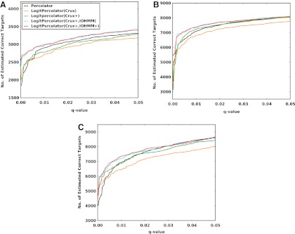
FDR curves; Train on SO-DR dataset, apply on top-ranking targets/decoys from Crux; LogitPercolator: our implementation of Percolator using Logistic Regression Classifier; Percolator: original Percolator; Crux: heuristics from Crux {XCorr, deltaCn, SpScore}; Crux+: heuristics [Crux, fracMatch (fraction of peptide fragments observed), fracExp (fraction of explained spectrum intensity)]; IOHMM: heuristics {Crux+, CSPI_Score^b, CSPI_Score^y}; IOHMM+: heuristics {IOHMM, delta_CSPI_Score^b, delta_CSPI_Score^y}, where delta is the difference between scores from top-ranking and the next best peptide (from original crux ranking); (A) 18Mix1_LCQ, Window-normalization; (B) 18Mix1_LTQ, Window-normalization; (C) Yeast_LTQ, Window-normalization. Interpretation is the same as for Figure 4.

Discussion

Scoring and confident identification of peptides is at the heart of mass spectrometry-based proteomics. In this article, we develop and test a novel and robust scoring algorithm based on learning peptide fragmentation from a large dataset of previously confidently identified peptides. Our framework is highly flexible and scalable, and can exploit different representations of PSM features in order to learn complex underlying patterns.

Using our prototype system, we have experimented with different pre-processing and normalization protocols, including a global rank-based method and a more local window-based method. Differences in these steps can dramatically alter the performance of the scoring system. Our results suggest that local normalization schemes may be superior to global approaches, possibly due the fact that different regions of the m/z range of MS/MS spectra show wide variability in both the density as well as intensity of peaks. This is well established in the literature, specifically for ion-trap data, where more and abundant peaks are generally observed from the middle of the peptides. Although our window-norm procedure is conceptually reasonable and achieves good performance, we acknowledge the existence of several pre-processing methods in the literature, (for example, Renard et al., 2009), that could be worth investigating within the CSPI framework.

With a good choice of features representing the problem at hand, machine learning methods have the potential to learn complex patterns even with noisy data like that obtained from MS/MS experiments. Incorporating several peptide properties in our models, we have shown how arbitrary features can be easily plugged into and tested with the CSPI framework. Although we have not evaluated each feature individually, the prototype appears to model y-ion intensities well, providing good discrimination between correct and incorrect peptides. The b-ion models clearly need additional fine-tuning of input layer features, normalization or both. From our experience, one reason for inadequate performance of b-ion models is the nature of the datasets used. Specifically, for ion-trap data from trypsin-digested proteins, y-ions are preferably more abundant in number and intensity than b-ions, which, in many cases, are much harder to discriminate from random noise matches. For most correctly identified peptides, several fragments from at least one ion-series (b- or y-) are observed. Since this information is lost when each ion-series is modeled separately, it might be beneficial to build joint models from b- and y-ion series.

Due to above factors, the composite score obtained by simple addition which gives equal weight to scores from b-ion and y-ion models does not optimally combine the evidence. In order to account for that as well as to take advantage of other available heuristics of PSM quality, we utilized LogitPercolator, a post hoc heuristic score combination tool based on the recent Percolator algorithm. Our results provide evidence suggesting that: i) IOHMMs provide a useful framework for modeling peptide fragmentation behavior and ii) intensity-based modeling can significantly improve peptide identification accuracies over current state-of-the-art.

In the current study, we have focused on a constrained set of peptides. However, the methods developed are general and can be extended to other precursor charge states, protein digestion enzymes, fragmentation protocols, or types of mass spectrometer, the only requirement being availability of validated (high-confidence) training data. These avenues will be explored in the future on diverse datasets for training and testing. Our prototype system is currently implemented as a set of stand-alone python scripts that allow creating FASTA database indexes, searching/scoring candidate peptides, re-scoring Crux results using IOHMM models and score combination using LogitPercolator. We have also implemented a multiprocessing version that can take advantage of multiple processors/cores on a computer system (if available) for computational speed-up. These scripts are available from authors upon request. Future work includes plans to develop software based on these scripts, which can be easily incorporated into established systems permitting broad distribution of our modeling framework.

Abbreviations Used

CFV

cross-fold validation.

CID

collision-induced dissociation

CSPI

context-sensitive peptide identification

FDR

false discovery rate

GEM

generalized expectation maximization

HMM

Hidden Markov Models

IO-HMM

Input-Output Hidden Markov Models

MS/MS

tandem mass spectrometry

PSM

peptide-spectrum match

SVM

support vector machine

Acknowledgments

We thank Dr. Vicky H. Wysocki for providing tandem MS data (SO-DR). We thank Drs. David Tabb and Michael MacCoss for useful comments and suggestions on the experiments and manuscript. We are also greatful to the Pittsburgh Supercomputing Center for providing computational resources. This work was supported in part by Grant numbers K25GM071951 from the NIGMS and RO1LM010950 from the NLM at the National Institutes of Health.

Author Disclosure Statement

No competing financial interests exist.

References

- Aebersold R. Goodlett DR. Mass spectrometry in proteomics. Chem Rev. 2001;101:269–295. doi: 10.1021/cr990076h. [DOI] [PubMed] [Google Scholar]
- Bengio Y. Frasconi P. Advances in Neural Information Processing Systems. The MIT Press; Cambridge, MA: 1995. An Input Output HMM Architecture; pp. 427–434. [Google Scholar]
- Bengio Y. Lauzon V-P. Ducharme RJ. Experiments on the application of IOHMMs to model financial returns series. IEEE Trans Neural Networks. 2001;12:113–123. doi: 10.1109/72.896800. [DOI] [PubMed] [Google Scholar]
- Bishop C. Neural Networks for Pattern Recognition. Oxford University Press; New York: 1996. [Google Scholar]
- Breci LA. Tabb DL. Yates JR., 3rd Wysocki VH. Cleavage N-terminal to proline: Analysis of a database of peptide tandem mass spectra. Anal Chem. 2003;75:1963–1971. doi: 10.1021/ac026359i. [DOI] [PubMed] [Google Scholar]
- Cortes C. Vapnik V. Support-vector networks. Machine Learning. 1995;20:273–297. [Google Scholar]
- Craig R. Beavis RC. TANDEM: Matching proteins with tandem mass spectra. Bioinformatics. 2004;20:1466–1467. doi: 10.1093/bioinformatics/bth092. [DOI] [PubMed] [Google Scholar]
- Craig R. Cortens JP. Beavis RC. Open source system for analyzing, validating, and storing protein identification data. J Proteome Res. 2004;3:1234–1242. doi: 10.1021/pr049882h. [DOI] [PubMed] [Google Scholar]
- Dempster LN. Rubin DB. Maximum likelihood from incomplete data via the EM algorithm. J Royal Stat Soc. 1977;39:1–38. [Google Scholar]
- Desiere F. Deutsch EW. King NL. Nesvizhskii AI. Mallick P. Eng J, et al. The PeptideAtlas project. Nucleic Acids Res. 2006;34(Database issue):D655–658. doi: 10.1093/nar/gkj040. [DOI] [PMC free article] [PubMed] [Google Scholar]
- Elias JE. Gibbons FD. King OD. Roth FP. Gygi SP. Intensity-based protein identification by machine learning from a library of tandem mass spectra. Nat Biotechnol. 2004;22:214–219. doi: 10.1038/nbt930. [DOI] [PubMed] [Google Scholar]
- Eng J. Mccormack A. Yates J. An approach to correlate tandem mass spectral data of peptides with amino acid sequences in a protein database. J Am Soc Mass Spectrom. 1994;5:976–989. doi: 10.1016/1044-0305(94)80016-2. [DOI] [PubMed] [Google Scholar]
- Geer LY. Markey SP. Kowalak JA. Wagner L. Xu M. Maynard DM, et al. Open mass spectrometry search algorithm. J Proteome Res. 2004;3:958–964. doi: 10.1021/pr0499491. [DOI] [PubMed] [Google Scholar]
- Grover H. University of Pittsburgh; 2012. Context-sensitive Markov models for peptide scoring and identification from tandem mass spectrometry. Ph.D. Thesis. [DOI] [PMC free article] [PubMed] [Google Scholar]
- Grover H. Gopalakrishnan V. Efficient processing of models for large-scale shotgun proteomics data. International Workshop on Collaborative Big Data. 2012 doi: 10.4108/icst.collaboratecom.2012.250716. [DOI] [PMC free article] [PubMed] [Google Scholar]
- Huang Y. Tseng GC. Yuan S. Pasa-Tolic L. Lipton MS. Smith RD, et al. A data-mining scheme for identifying peptide structural motifs responsible for different MS/MS fragmentation intensity patterns. J Proteome Res. 2008;7:70–79. doi: 10.1021/pr070106u. [DOI] [PMC free article] [PubMed] [Google Scholar]
- Hubbard SJ. Jones AR. Gucinski AC. Dodds ED. Li W. Wysocki VH. Understanding and exploiting peptide fragment ion intensities using experimental and informatic approaches. Proteome Bioinformatics. 2010;604:73–94. doi: 10.1007/978-1-60761-444-9_6. Human Press. [DOI] [PubMed] [Google Scholar]
- Jensen FV. Nielsen TD. Bayesian networks and decision graphs. 2nd. Springer; New York: 2007. [Google Scholar]
- Kall L. Canterbury JD. Weston J. Noble WS. Maccoss MJ. Semi-supervised learning for peptide identification from shotgun proteomics datasets. Nat Methods. 2007;4:923–925. doi: 10.1038/nmeth1113. [DOI] [PubMed] [Google Scholar]
- Kall L. Storey JD. Maccoss MJ. Noble WS. Assigning significance to peptides identified by tandem mass spectrometry using decoy databases. J Proteome Res. 2008;7:29–34. doi: 10.1021/pr700600n. [DOI] [PubMed] [Google Scholar]
- Keller A. Nesvizhskii AI. Kolker E. Aebersold R. Empirical statistical model to estimate the accuracy of peptide identifications made by MS/MS and database search. Anal Chem. 2002;74:5383–5392. doi: 10.1021/ac025747h. [DOI] [PubMed] [Google Scholar]
- Khatun J. Hamlett E. Giddings MC. Incorporating sequence information into the scoring function: A hidden Markov model for improved peptide identification. Bioinformatics. 2008;24:674–681. doi: 10.1093/bioinformatics/btn011. [DOI] [PMC free article] [PubMed] [Google Scholar]
- Klammer AA. Reynolds SM. Bilmes JA. Maccoss MJ. Noble WS. Modeling peptide fragmentation with dynamic Bayesian networks for peptide identification. Bioinformatics. 2008;24:i348–356. doi: 10.1093/bioinformatics/btn189. [DOI] [PMC free article] [PubMed] [Google Scholar]
- Li W. Ji L. Goya J. Tan G. Wysocki VH. SQID: An intensity-incorporated protein identification algorithm for tandem mass spectrometry. J Proteome Res. 2011;10:1593–1602. doi: 10.1021/pr100959y. [DOI] [PMC free article] [PubMed] [Google Scholar]
- Marcotte E. How do shotgun proteomics algorithms identify proteins? Nature Biotechnol. 2007;25:755–757. doi: 10.1038/nbt0707-755. [DOI] [PubMed] [Google Scholar]
- Marshall AG. Hendrickson CL. Jackson GS. Fourier transform ion cyclotron resonance mass spectrometry: A primer. Mass Spectrom Rev. 1998;17:1–35. doi: 10.1002/(SICI)1098-2787(1998)17:1<1::AID-MAS1>3.0.CO;2-K. [DOI] [PubMed] [Google Scholar]
- Martens L. Hermjakob H. Jones P. Adamski M. Taylor C. States D, et al. PRIDE: The proteomics identifications database. Proteomics. 2005;5:3537–3545. doi: 10.1002/pmic.200401303. [DOI] [PubMed] [Google Scholar]
- Murphy K. UC Berkeley: 2002. Dynamic Bayesian networks: Representation, inference and learning. Ph.D. Thesis. [Google Scholar]
- Nesvizhskii AI. Protein identification by tandem mass spectrometry and sequence database searching. Methods Mol Biol. 2007;367:87–119. doi: 10.1385/1-59745-275-0:87. [DOI] [PubMed] [Google Scholar]
- Nesvizhskii AI. Vitek O. Aebersold R. Analysis and validation of proteomic data generated by tandem mass spectrometry. Nat Methods. 2007;4:787–797. doi: 10.1038/nmeth1088. [DOI] [PubMed] [Google Scholar]
- Paizs B. Suhai S. Fragmentation pathways of protonated peptides. Mass Spectrom Rev. 2005;24:508–548. doi: 10.1002/mas.20024. [DOI] [PubMed] [Google Scholar]
- Park CY. Klammer AA. Kall L. Maccoss MJ. Noble WS. Rapid and accurate peptide identification from tandem mass spectra. J Proteome Res. 2008;7:3022–3027. doi: 10.1021/pr800127y. [DOI] [PMC free article] [PubMed] [Google Scholar]
- Perkins DN. Pappin DJ. Creasy DM. Cottrell JS. Probability-based protein identification by searching sequence databases using mass spectrometry data. Electrophoresis. 1999;20:3551–3567. doi: 10.1002/(SICI)1522-2683(19991201)20:18<3551::AID-ELPS3551>3.0.CO;2-2. [DOI] [PubMed] [Google Scholar]
- Rabiner L. A tutorial on hidden Markov models and selected applications in speech recognition. Proceedings of the IEEE. 1989;77:257–286. [Google Scholar]
- Renard BY. Kirchner M. Monigatti F. Ivanov AR. Rappsilber J. Winter D, et al. When less can yield more. Computational preprocessing of MS/MS spectra for peptide identification. Proteomics. 2009;9:4978–4984. doi: 10.1002/pmic.200900326. [DOI] [PubMed] [Google Scholar]
- Searle BC. Turner M. Nesvizhskii AI. Improving sensitivity by probabilistically combining results from multiple MS/MS search methodologies. J Proteome Res. 2008;7:245–253. doi: 10.1021/pr070540w. [DOI] [PubMed] [Google Scholar]
- Steen H. Mann M. The ABC's (and XYZ's) of peptide sequencing. Nat Rev Mol Cell Biol. 2004;5:699–711. doi: 10.1038/nrm1468. [DOI] [PubMed] [Google Scholar]
- Tabb DL. Fernando CG. Chambers MC. MyriMatch: Highly accurate tandem mass spectral peptide identification by multivariate hypergeometric analysis. J Proteome Res. 2007;6:654–661. doi: 10.1021/pr0604054. [DOI] [PMC free article] [PubMed] [Google Scholar]
- Tabb DL. Huang Y. Wysocki VH. Yates JR., 3rd Influence of basic residue content on fragment ion peak intensities in low-energy collision-induced dissociation spectra of peptides. Anal Chem. 2004;76:1243–1248. doi: 10.1021/ac0351163. [DOI] [PMC free article] [PubMed] [Google Scholar]
- Tsaprailis G. Nair H. Zhong W. Kuppannan K. Futrell JH. Wysocki VH. A mechanistic investigation of the enhanced cleavage at histidine in the gas-phase dissociation of protonated peptides. Anal Chem. 2004;76:2083–2094. doi: 10.1021/ac034971j. [DOI] [PMC free article] [PubMed] [Google Scholar]
- Vaisar T. Urban J. Probing the proline effect in CID of protonated peptides. J Mass Spectrom. 1996;31:1185–1187. doi: 10.1002/(SICI)1096-9888(199610)31:10<1185::AID-JMS396>3.0.CO;2-Q. [DOI] [PubMed] [Google Scholar]
- Vapnik VN. Statistical learning theory. Wiley; New York: 1998. [DOI] [PubMed] [Google Scholar]
- Vitek O. Getting started in computational mass spectrometry-based proteomics. PLoS Comput Biol. 2009;5:e1000366. doi: 10.1371/journal.pcbi.1000366. [DOI] [PMC free article] [PubMed] [Google Scholar]
- Wan Y. Yang A. Chen T. PepHMM: A hidden Markov model based scoring function for mass spectrometry database search. Anal Chem. 2006;78:432–437. doi: 10.1021/ac051319a. [DOI] [PubMed] [Google Scholar]
- Wilm M. Principles of electrospray ionization. Mol Cell Proteomics. 2011;10:M111 009407. doi: 10.1074/mcp.M111.009407. [DOI] [PMC free article] [PubMed] [Google Scholar]
- Wysocki VH. Tsaprailis G. Smith LL. Breci LA. Mobile and localized protons: A framework for understanding peptide dissociation. J Mass Spectrom. 2000;35:1399–1406. doi: 10.1002/1096-9888(200012)35:12<1399::AID-JMS86>3.0.CO;2-R. [DOI] [PubMed] [Google Scholar]
- Zhou C. Bowler LD. Feng J. A machine learning approach to explore the spectra intensity pattern of peptides using tandem mass spectrometry data. BMC Bioinform. 2008;9:325–341. doi: 10.1186/1471-2105-9-325. [DOI] [PMC free article] [PubMed] [Google Scholar]
Associated Data
This section collects any data citations, data availability statements, or supplementary materials included in this article.