Simple electrolyte solutions: Comparison of DRISM and molecular dynamics results for alkali halide solutions

Abstract

Using the dielectrically consistent reference interaction site model (DRISM) of molecular solvation, we have calculated structural and thermodynamic information of alkali-halide salts in aqueous solution, as a function of salt concentration. The impact of varying the closure relation used with DRISM is investigated using the partial series expansion of order-n (PSE-n) family of closures, which includes the commonly used hypernetted-chain equation (HNC) and Kovalenko-Hirata closures. Results are compared to explicit molecular dynamics (MD) simulations, using the same force fields, and to experiment. The mean activity coefficients of ions predicted by DRISM agree well with experimental values at concentrations below 0.5 m, especially when using the HNC closure. As individual ion activities (and the corresponding solvation free energies) are not known from experiment, only DRISM and MD results are directly compared and found to have reasonably good agreement. The activity of water directly estimated from DRISM is nearly consistent with values derived from the DRISM ion activities and the Gibbs-Duhem equation, but the changes in the computed pressure as a function of salt concentration dominate these comparisons. Good agreement with experiment is obtained if these pressure changes are ignored. Radial distribution functions of NaCl solution at three concentrations were compared between DRISM and MD simulations. DRISM shows comparable water distribution around the cation, but water structures around the anion deviate from the MD results; this may also be related to the high pressure of the system. Despite some problems, DRISM-PSE-n is an effective tool for investigating thermodynamic properties of simple electrolytes.

INTRODUCTION

Physiological fluids always include various ions, and the biological activity of biomolecules cannot be understood separately without knowing their interactions with these ions. Computational simulation is a convenient tool for studying electrolyte solutions and visualizing their behavior at atomistic resolution. Implicit solvent models can be a useful alternative because they save considerable computational time. One popular approach treats water as a dielectric continuum augmented by a continuous charge distribution to represent mobile co- and counter-ions (as in the original Debye-Hückel theory). The generalized Born^{1, 2, 3} and Poisson-Boltzmann models^{4, 5, 6} belong to this category. However, these models fail to describe atomistic details of the solvent molecules and only provide rough estimates of the thermodynamics of the system. The integral equation approach of Ornstein and Zernike^{7, 8, 9} offers an implicit approach that maintains the atomic and molecular nature of the solvent. In particular, the reference interaction site model (RISM)¹⁰ and its variants^{11, 12} are often used to apply integral equation models to molecular solvents such as water. Because of its computational efficiency, the RISM theory is capable of exploring a wide range of temperatures, pressures, and densities. The rich set of thermodynamic data that can be extracted from RISM solutions makes it an ideal choice to study a wide range of complex liquids, including ionic liquids^{13, 14, 15} and bitumen.¹⁶ Furthermore, characterizations of bulk liquids provided by RISM are commonly used with 3D-RISM^{17, 18, 19, 20} to provide detailed solvent distributions and thermodynamics for complex macromolecules.^{21, 22, 23}

Several variations of RISM theory exist (we use “RISM” to refer to them generally unless otherwise noted). As the original RISM theory¹⁰ was unsuitable for the study of charged or polar molecules, extended RISM (XRISM)^{11, 24, 25} was developed to treat realistic models of water and ions at infinite dilution.^{26, 27} However, XRISM gives a trivial dielectric constant that is far too low compared to experiment.²⁸ Besides the obvious physical concerns, the low dielectric constant caused difficulties converging finite concentration salt solutions. The so-called ARISM correction used a coefficient, ‘A,’ to scale electrostatic interactions and impose a desired dielectric constant.²⁹ This preceded the development of XRISM but this approach led to inconsistencies when finite concentrations of salt were used.³⁰ This motivated the development of dielectrically consistent RISM (DRISM),^{12, 31} which enforces the desired dielectric constant for all thermodynamic routes. The amount of thermodynamic data available from solving these equations has also increased over time with the use of analytic and finite difference thermodynamic derivatives. Specifically, pressure,³² temperature,³³ and density derivatives³⁴ have given expressions for partial molar compressibility, solvation energy, and solvation entropy.

In addition to the RISM equation, an approximate closure equation is required to obtain a solution. Historically, the hyper-netted chain equation (HNC)³⁵ has been the most popular, especially for systems with strong electrostatic interactions. Recently, some studies^{36, 37} have had success with the Kovalenko-Hirata (KH) closure,¹⁹ which also has better convergence properties. The partial series expansion of order-n (PSE-n) closure,³⁸ which interpolates between HNC and KH, has since been developed. Also of interest are closures with non-trivial dielectric constants.^{39, 40} These were developed as alternatives to DRISM, but have not been as widely used.

Using XRISM, ARISM, and DRISM, ion hydration, and bulk aqueous ionic solutions have been studied in both the infinite dilution regime^{27, 32, 33, 34, 38, 41, 42, 43, 44, 45, 46} and over a range of finite salt concentrations.^{12, 30, 31, 36, 37, 47, 48, 49, 50, 51, 52} These studies have used a number of different of water and ion models to explore a wide range of physical conditions. This includes extreme temperatures,^{47, 48, 51, 52} pressures,^{51, 52} and concentrations.⁴⁹

A wealth of information has been calculated from these studies. Radial distribution functions (RDFs) are the primary result of RISM, which thermodynamic parameters can be derived from. A rather direct transformation yields potentials of mean force (PMFs)^{12, 27, 30, 31, 34, 49, 53} and coordination numbers.⁵⁰ Combining RDFs with the direct correlation function, solvation free energies (excess chemical potentials)^{30, 33, 34, 37, 41, 42, 44, 45, 46} may be calculated and be decomposed into entropies,^{30, 33, 34, 41, 45, 46} energies,^{30, 33, 34, 41, 45, 46} enthalpies,^{33, 45} and polar/non-polar⁴⁵ contributions. Mean ionic activity coefficients have been calculated for a few ion models using Kirkwood-Buff theory^{12, 31} and excess chemical potential formulations.³⁶ Partial molar volumes^{32, 41} and compressibilities³² have been calculated and radially decomposed for monovalent alkali-halide ions. The solubility of both ions⁴⁹ and non-polar molecules⁵⁰ in salt solutions has been examined. The electrostatic properties of ions at infinite dilution have examined in terms of radial decomposition of effective electrostatic potentials,^{43, 44} dielectric susceptibility,⁴⁴ and the screening factor.⁴⁴

From this data, a picture emerges of DRISM providing a qualitatively correct description of aqueous ionic solutions. For all of the models used, DRISM correctly shows the asymmetry in multiple properties for the hydration of anions and cations. When RDFs have been compared against simulation data, they have had largely the correct structure, including multiple minima in the anion-cation PMFs, a property of molecular hydration. Mean activity coefficients also show a distinct improvement over linearized Debye-Hückel theory, though the limited data available indicate this may be sensitive to the ion parameters used.

Given the increasing popularity of 3D-RISM, there remain a number of important questions about the DRISM representation of salt solution. A primary issue is the selection of water and ion force field parameters and closures. Water and ion models used in the aforementioned studies have often been mixtures of different parametrizations with unknown behavior when used with molecular dynamics or Monte Carlo methods. Furthermore, comparison to experiment and simulation has been limited. To assess the quality of the theory, it is necessary to know the performance of the force field, which requires comparing to simulation and experiment simultaneously. At the same time, no studies have systematically investigated the effect of closure approximations or attempted to compare existing closures. Finally, the HNC family of closures has long been known to have limited thermodynamic consistency (i.e., virial-energy, but not compressibility-energy),^{54, 55, 56, 57} but recently, it has been suggested³⁷ that DRISM-HNC itself may not have even this limited consistency.

To address these issues, we have used DRISM to calculate equilibrium properties of several combinations of alkali and halide ions and tested thermodynamic consistency via the Gibbs-Duhem relation. Importantly, we have used the Joung-Cheatham⁵⁸ SPC/E parameter set for monovalent ions,⁵⁸ which has been shown to be in good quantitative agreement with experiment.^{58, 59, 60, 61} Throughout, we have used KH, PSE-n, and HNC closures and compared, wherever possible, DRISM, molecular dynamics, and experiment. This approach allows us to decouple the theory from the input model and critically assess the results.

The remainder of this paper is organized as follows. In Sec. 2, we summarize details of the DRISM theory and the calculation of thermodynamics from its solution. In Sec. 3, we describe the DRISM and molecular dynamics calculations. Results of these calculations are compared to experiment in Sec. 4. Section 5 presents our conclusions.

THEORY

The RISM and DRISM models

The RISM equation is also called the site-site Ornstein-Zernike (OZ)^{7, 8, 9} equation. Solving the original OZ equation with a complementary closure equation gives two correlation functions, the direct and total correlation functions, between any two particles (or sites) in the system. The original OZ approach dealt only with spherical molecules with no orientational dependence. Multiple-site molecules, such as water, introduce orientational degrees of freedom to the correlation functions. Due to the extra dimensions, solving the OZ equation with explicit orientational dependency^{62, 63} is not trivial and its application is limited.

The RISM equation averages the orientations of multiple-site molecules such that the correlation functions depend only on the distance between two molecular sites.^{10, 11} According to the theory, the total correlation function h and direct correlation function c between two sites can be related by the equation

$$\begin{array}{ccc}\hfill h_{\alpha \gamma }\left(r\right)& =& \sum _{\lambda }^{N_{\text{site}}}\sum _{\beta }^{N_{\text{site}}}{\omega }_{\alpha \lambda }\left(r\right)*c_{\lambda \beta }\left(r\right)*{\omega }_{\beta \gamma }\left(r\right)\hfill \\ & & +\sum _{\lambda }^{N_{\text{site}}}\sum _{\beta }^{N_{\text{site}}}{\omega }_{\alpha \lambda }\left(r\right)*c_{\lambda \beta }\left(r\right)*{\rho }_{\beta }{h}_{\beta \gamma }\left(r\right).\hfill \end{array}$$ (1)

Subscripts with Greek letters represent specific sites of molecules and ω is the intramolecular correlation function. Asterisks stand for a convolution integral over the whole real space. This can be rewritten in the simpler matrix form

$$\begin{array}{ccc}\hfill \mathbf{h}& =& \mathit{\omega }*\mathbf{c}*\mathit{\omega }+\mathit{\omega }*\mathbf{c}*\mathit{\rho }\mathbf{h}\hfill \\ & =& {[\mathbf{1}-\mathit{\omega }*\mathbf{c}\mathit{\rho }]}^{-1}\mathit{\omega }*\mathbf{c}*\mathit{\omega }.\hfill \end{array}$$ (2)

Convolutions are calculated in reciprocal-space via the Fourier transform.

Equation 2 cannot be solved by itself because there are two unknowns, h and c. To close the equation, another equation is introduced. A general form of the closure equation is

$$\begin{array}{c}\hfill g_{\alpha \gamma }\left(r\right)=\exp \{-\beta u_{\alpha \gamma }\left(r\right)+h_{\alpha \gamma }\left(r\right)-c_{\alpha \gamma }\left(r\right)+b_{\alpha \gamma }\left(r\right)\},\end{array}$$ (3)

where u is the pair potential and β = 1/k_BT. b is called the bridge function, and various functional forms of b have been studied.^{17, 64} One of the most popular approximations assumes b = 0, giving the hyper-netted chain (HNC) equation³⁵

$$\begin{array}{c}\hfill g_{\alpha \gamma }\left(r\right)=\exp \{-\beta u_{\alpha \gamma }\left(r\right)+h_{\alpha \gamma }\left(r\right)-c_{\alpha \gamma }\left(r\right)\}.\end{array}$$ (4)

The combination of Eqs. 2, 4 describes systems with long-range interactions well, but it can be difficult to converge solutions. The KH closure¹⁹ was devised to overcome the difficulty, and does so by partially linearizing the right-hand side of Eq 4. Later, the KH closer was further generalized by Kast and Kloss³⁸ to give the PSE-n closure,

$$g_{\alpha \gamma }\left(r\right)=\left\{\begin{array}{cc}\hfill \exp \left\{t_{\alpha \gamma }^{*}\left(r\right)\right\}& \hfill \text{for}{t}_{\alpha \gamma }^{*}\left(r\right)<0\\ \hfill \sum _{i=0}^n\frac{{\left(t_{\alpha \gamma }^{*}\left(r\right)\right)}^i}{i!}& \hfill \text{for}{t}_{\alpha \gamma }^{*}\left(r\right)\ge 0,\end{array}\right.$$ (5)

$$t_{\alpha \gamma }^{*}\left(r\right)=-\beta u_{\alpha \gamma }\left(r\right)+h_{\alpha \gamma }\left(r\right)-c_{\alpha \gamma }\left(r\right).$$

When n = 1, it is equivalent to the KH closure. When n = ∞, it yields the HNC closure.

It is known that dielectric constants calculated from the solutions of Eqs. 1, 4 are generally very low and inconsistent with the behavior of water.^{12, 31} The deviation was presumed to be caused by the inappropriate long-ranged behavior of polar molecules. Perkyns and Pettitt³⁰ proposed the dielectrically consistent RISM (DRISM) as a remedy for the problem.¹² They introduced a bridge-like correction ζ to Eq. 2

$${\mathbf{h}}^{\prime }={[\mathbf{1}-{\mathit{\omega }}^{\prime }*\mathbf{c}]}^{-1}{\mathit{\omega }}^{\prime }*\mathbf{c}*{\mathit{\omega }}^{\prime },$$ (6)

where h′ = h − ζ and ω′ = ω + ζ. Here, ζ is determined by the desired dielectric constant, which is now an input parameter.

One major advantage of the RISM theory compared to continuum solvent models is that one can obtain atomistic details or correlation functions as the results of the RISM calculation. Therefore, the results can be easily compared to the results of all-atom MD or Monte Carlo simulations. Popular all-atom simulations usually determine the energy of the system by summing pair-wise site-site interaction energies. Therefore, the potential energy model itself can be shared with the RISM theory. The pair-wise non-bond energy is most often expressed by the summation of Coulombic potential energy and van der Waals (vdW) potential, which is represented by a Lennard-Jones (LJ) potential.

$$u_{\alpha \gamma }\left(r\right)=\frac{q_{\alpha }{q}_{\gamma }}{r}+{\varepsilon }_{\alpha \gamma }\left[{\left(\frac{R_{\text{min,}\alpha \gamma }}{r}\right)}^{12}-2{\left(\frac{R_{\text{min,}\alpha \gamma }}{r}\right)}^6\right],$$

where q's are charges of sites, and ɛ and R_min are Lennard-Jones parameters of the pair. (See the Appendix: Long-range Coulomb Interactions) With the exact closure, the correlation functions calculated by the RISM theory should be nearly identical to the MD simulations results. Exact reproduction of MD results is also limited by approximations to the direct correlation function and orientational averaging.⁶⁵ However, comparisons between RISM theory and molecular Ornstein-Zernike^{7, 8, 9} suggest that approximations to the closure relation, and not orientional averaging, are the principle source of error.^{66, 67}

Chemical potentials

The molar solvation free energy is equivalent to the excess chemical potential, μ_ex, in aqueous solution; see the Appendix for a discussion. μ_ex can be expressed by the difference of the interaction energies of the two end-states with and without the inserted particle (ΔU). If ∂U/∂λ is evaluated at every intermediate state, thermodynamic integration (TI) can also lead to the same chemical potential.⁶⁸ If λ is scaled from 0 to 1, the equation becomes

$${\mu }_{\text{ex}}={\int }_0^1⟨\frac{\partial U\left(\lambda \right)}{\partial \lambda }⟩d\lambda .$$ (7)

For the RISM, the Kirkwood formula can be conveniently used to calculate the excess chemical potential because the radial distribution functions are known from the solution. For a solute site, α,

$${\mu }_{\text{ex,}\alpha }=\sum _{\gamma }{\rho }_{\gamma }{\int }_0^1\left[4\pi {\int }_0^{\infty }\frac{\partial u_{\alpha \gamma }\left(r;\lambda \right)}{\partial \lambda }{g}_{\alpha \gamma }\left(r;\lambda \right)r^{2}dr\right]d\lambda .$$ (8)

For RISM with HNC-like closures (Eq. 5), this equation can be solved analytically^{19, 38, 69}

$$\begin{array}{ccc}\hfill {\mu }_{\text{ex,}\alpha }& =& 4\pi k_{b}T\sum _{\gamma }{\rho }_{\gamma }{\int }_0^{\infty }\hfill \\ & & \times \left[\frac{h_{\alpha \gamma }^2}{2}-c_{\alpha \gamma }-\frac{h_{\alpha \gamma }{c}_{\alpha \gamma }}{2}-\frac{{\left(t_{\alpha \gamma }^{*}\right)}^{n+1}}{(n+1)!}\Theta \left(t_{\alpha \gamma }^{*}\right)\right]r^{2}dr.\hfill \end{array}$$ (9)

As with Eq. 5, n = 1 yields the excess chemical potential for the KH closure while n = ∞ gives the HNC result.

Equation 9 has been derived for RISM, and is not strictly valid for DRISM. Furthermore, μ_ex is not known to be stationary with respect to h and c in the DRISM theory, so there is no equivalent expression for DRISM and μ_ex may not be a path-independent state function in the theory.³⁷ That said, Eq. 9 has been extensively used in the literature with DRISM for the past two decades, and is known to produce useful results. Some examples from the literature include Perkyns and Pettitt,³⁰ Kinoshita and Hirata,⁵⁰ Yoshida et al.,³⁶ and Schmeer and Maurer.³⁷ Since Eq. 9 is not the exact expression for DRISM, it may be considered an approximate expression for the excess chemical potential. Explicit use of approximate expressions has also been used frequently in the literature to either calculate excess chemical potential where no expression exists,⁶⁴ or to provide possibly more accurate results compared to experiment.^{42, 70, 71, 72, 73} Other forms for the excess chemical potential, specifically the hc/2 term, can be found in the literature,^{37, 69} which give slightly different numerical results when used with DRISM. The differences among them are minor compared to the absolute excess chemical potential. However, the numerical results from the various formulas are not different when used with XRISM.

The Gibbs-Duhem relations

The activity coefficient and excess chemical potential of the ion are closely related experimental observables that depend both on the specific properties and concentration of the ions involved,

$$k_{B}T\ln {\gamma }_m=k_{B}T\ln \frac{{\rho }_w}{{\rho }_{w,\infty }}+\Delta {\mu }_{\text{ex}},$$

where ∞ denotes the infinitely dilute state, ρ_w is the number density of the solvent (water) and Δμ_ex = μ_ex − μ_ex,∞. At infinite dilution state, γ_m goes to unity. Note that the activity coefficient γ_m is in the scale of molal concentration (m) of the solute. Other scales result in slightly different formulas (see the Appendix). Individual activities of the dissolved ions of a neutral salt are not available in a model-free way from experiment, and, thus, the mean activity coefficient (γ_±) is often employed,

$$\nu k_{B}T\ln {\gamma }_{m,\pm }=k_{B}T\ln \frac{{\rho }_w}{{\rho }_{w,\infty }}+\sum _i{s}_i\Delta {\mu }_{\text{ex},i},$$ (10)

where s_i is the number of generated free ions of species i when a single salt molecule is dissolved and ν = ∑s_i. (For the simple salts considered here, s_i = 1 and ν = 2.)

Theoretical predictions of activity coefficients can be calculated via a number of methods. For RISM calculations, Eq. 9 can be directly inserted into Eq. 10. Though obtaining the excess chemical potential from MD simulations is straightforward using thermodynamic integration (see Sec. 3B), it is generally not possible to calculate the infinite dilution limit, necessary in Eq. 10. Furthermore, low salt-concentration (<10 mM) simulations are prohibitively expensive to compute. A third, simple approach commonly used is the Debye-Hückel limiting law,⁷⁴ which theoretically estimates mean activity coefficients of salts at low concentrations,

$$\ln {\gamma }_{m,\pm }=-A_{\text{DH}}\left(\prod _i{s}_i\right){\left[\frac{1}{2}\sum _i{s}_i^2{m}_i\right]}^{1/2},$$ (11)

where the Debye-Hückel constant A_DH is 1.1724 kg^1/2mol^−1/2 at 298 K.⁷⁵

The Gibbs-Duhem relation links the excess chemical potential of the solvent and ions with the total pressure,

$${\rho }_{w}d{\mu }_w+\sum _i{\rho }_{i}d{\mu }_i=dp.$$ (12)

In the equation, the term for water is separated to distinguish it from other ionic components and the summation in the second term is only for ionic components. As DRISM-PSE-n is thought to be thermodynamically inconsistent, the Gibbs-Duhem relation can be used to provide a measure of this inconsistency. To do this, we would like to express Δμ_{ex, w} in terms of Δμ_{ex, ions}.

First, the chemical potentials can be divided into their “ideal” and “excess” portions,

$$\begin{array}{c}\hfill {\rho }_{w}d{\mu }_{\text{ideal,}w}+\sum _i{\rho }_{i}d{\mu }_{\text{ideal,}i}+{\rho }_{w}d{\mu }_{\text{ex,}w}+\sum _i{\rho }_{i}d{\mu }_{\text{ex,}i}=dp.\end{array}$$ (13)

Historically, there are a variety of definitions of μ_ideal of particle A. A derivation of μ_ideal from the ideal gas equation used by RISM yields

$${\mu }_{\text{ideal},A}=k_{B}T\ln {\Lambda }_A^3+k_{B}T\ln {\rho }_A,$$ (14)

where Λ is the thermal de Broglie wavelength, and is independent of the concentration of the particle. By simple rearrangement, Eq. 13 becomes

$$\begin{array}{cc}\hfill d{\mu }_{\text{ex,}w}& =\frac{1}{{\rho }_w}\left[-\sum _i{\rho }_{i}d{\mu }_{\text{ex,}i}+dp-k_{B}T\left(d{\rho }_w+\sum _{i}d{\rho }_i\right)\right]\hfill \\ & =d{\mu }_{\text{ex},w}^{\text{sol}}+d{\mu }^{\text{press}}+d{\mu }^{\rho },\hfill \end{array}$$ (15)

where we have used dμ_ideal = (k_bT/ρ)dρ. We can get Δμ_ex,w(m) = μ_ex,w(m) − μ_{ex, w, ∞} by integrating both sides from infinite dilution to concentration m,

$$\begin{array}{cc}\hfill \Delta {\mu }_{\text{ex,}w}& =\Delta {\mu }_{\text{ex,}w}^{\text{sol}}+\Delta {\mu }^{\text{press}}+\Delta {\mu }^{\rho }\hfill \end{array}$$ (16)

(see Sec. I of the supplementary material⁷⁶), where

$$\begin{array}{ccc}\hfill \Delta {\mu }_{\text{ex,}w}^{\text{sol}}& =& \frac{-M_w}{1000}\sum _i{s}_i\left(m\Delta {\mu }_{\text{ex,}i}\left(m\right)-{\int }_0^m\Delta {\mu }_{\text{ex,}i}\left(m^{\prime }\right)d{m}^{\prime }\right),\hfill \end{array}$$ (17)

$$\Delta {\mu }^{\text{press}}={\int }_{p_{\infty }}^p\frac{1}{{\rho }_w\left(p^{\prime }\right)}d{p}^{\prime },$$ (18)

and

$$\begin{array}{cc}\hfill \Delta {\mu }^{\rho }& =-k_{B}T\left[\ln \left(\frac{{\rho }_w}{{\rho }_{w,\infty }}\right)+\frac{\nu M_{w}m}{1000}\right].\hfill \end{array}$$ (19)

Δμ^press is contributed by the change of the system pressure. Since it is proportional to 1/ρ_w, the absolute contribution tends to be greater as the density of water gets smaller. If there is no pressure change, Δμ^press is zero. Δμ^ρ is the contribution from the change of water density and it is essentially zero if the water density is fixed. If the Gibbs-Duhem equation is strictly obeyed, the chemical potential difference calculated from Eq. 16 should match that calculated using Eq. 9.

In solution chemistry, a different definition of the ideal part of the chemical potential is used that depends on the units of concentration. For a mole-fraction scale,

$${\mu }_{\text{ideal,}A}^x={\mu }^{\circ }+k_{B}T\ln x_A,$$ (20)

where μ° is the chemical potential of the reference state. If A is the solvent, the reference state becomes pure A. If A is a solute, the reference state becomes the hypothetical pure solute. Now, we can relate the change of chemical potential of ions to the change of chemical potential of water using Eqs. 13, 20. If Eq. 20 is used, the ideal parts of the chemical potential become

$$\begin{array}{cc}\hfill {\rho }_{w}d{\mu }_{\text{ideal,}w}^x+\sum _i{\rho }_{i}d{\mu }_{\text{ideal,}i}^x& =k_{B}T\rho \left(d{x}_w+\sum _{i}d{x}_i\right)=0,\hfill \end{array}$$ (21)

where we have used ρ_w/x_w = ρ_i/x_i = ρ. In the above equation, the sum of the change of the mole fraction of the all the molecules in the system, (dx_w + ∑_idx_i), is always zero. Equation 12 can then be written in terms of the excess chemical potentials,

$${\rho }_{w}d{\mu }_{\text{ex,}w}^x+\sum _i{\rho }_{i}d{\mu }_{\text{ex,}i}^x=dp.$$ (22)

For typical experiments and MD simulations, dp = 0 and the equation can be rearranged for the excess chemical potential of water (μ_ex),

$$\begin{array}{cc}\hfill d{\mu }_{\text{ex,}w}^x& =\sum _i-s_{i}m\left(\frac{M_w}{1000}\right)\frac{d{\mu }_{\text{ex,}i}^x}{dm}dm,\hfill \end{array}$$ (23)

where M_w is the molecular weight of water. The difference of excess chemical potential of water between in a solution of molal concentration m of the salt and in pure water, $\Delta {\mu }_{\text{ex,}w}^x\left(m\right)={\mu }_{\text{ex,}w}^x\left(m\right)-{\mu }_{\text{ex},w,\infty }^x$, is obtained by integrating the equation above from infinite dilution to concentration m as in Eq. 17,

$$\begin{array}{ccc}\hfill \Delta {\mu }_{\text{ex,}w}^x\left(m\right)& =& \frac{-M_w}{1000}\sum _i{s}_i\left(m\Delta {\mu }_{\text{ex,}i}^x\left(m\right)\right.\hfill \\ & & \left.-{\int }_0^m\Delta {\mu }_{\text{ex,}i}^x\left(m^{\prime }\right)d{m}^{\prime }\right).\hfill \end{array}$$ (24)

Note that $\Delta {\mu }_{\text{ex,}i}^x$ is slightly different from Δμ_ex,i, as shown in Eq. B7 in the Appendix, although their differences are very small at low concentrations. Given ${\sum }_i{s}_i{\mu }_{\text{ex,}i}^x$ as a function of molal concentration of the salt, the integral in Eq. 24 can be determined by numerical integration. Equations 24, 17 are morphologically same but the definitions of the excess chemical potential are different. The ideal gas definition (Eq. 24) is useful since the resulting excess chemical potential is simply related to the transfer free energy from gas to liquid; the mole-fraction definition (Eq. 17) is generally used in experimental studies.

The activity of water (a_w) is obtained from the measured $\Delta {\mu }_{\text{ex,}w}^x$ by the definition of the chemical potential of water,

$$\ln a_w=\ln x_w+\frac{\Delta {\mu }_{\text{ex,}w}^x}{k_{B}T}.$$ (25)

The osmotic coefficient (ϕ) based on molality, which indicates the deviation from the ideality, is just a rearrangement of the water activity,

$$\varphi =-\frac{1000}{\nu m{M}_w}\ln a_w.$$ (26)

In most experiments, water activity is acquired by measuring vapor pressure of water and then the mean activity coefficient of ions are calculated from the Gibbs-Duhem relation. However, for simulations, measuring water activity is much harder because the change of chemical potential of the more populated water component is much smaller than for the ionic components, as Eq. 12 suggests. In RISM, the excess chemical potential of both water and ions can be directly calculated with Eq. 9.

Solvent pressure

The pressure of the system is related to the Helmholtz free energy (A),

$$p=\frac{G-A}{V}=-\frac{A}{V}+\sum _i^{\text{mol}}{\mu }_i{\rho }_i.$$ (27)

The Helmholtz free energy per volume for the PSE-n closure^{37, 38, 69, 77} is

$$\begin{array}{cc}\hfill \frac{A}{V}=& 2\pi \sum _{\alpha }^{N_{\text{site}}}\sum _{\gamma }^{N_{\text{site}}}{\rho }_{\alpha }{\rho }_{\gamma }{\int }_0^{\infty }\left(\frac{h_{\alpha \gamma }^2}{2}-c_{\alpha \gamma }-\frac{{\left(t_{\alpha \gamma }^{*}\right)}^{n+1}}{(n+1)!}\Theta \left(t_{\alpha \gamma }^{*}\right)\right)r^{2}dr\hfill \\ & +\frac{1}{{\left(2\pi \right)}^2}{\int }_0^{\infty }\{\text{Tr}\left(\mathit{\omega }\mathbf{c}\mathbf{\rho }\right)+\ln \det [\mathbf{1}-\mathit{\omega }\mathbf{c}\mathbf{\rho }]\}{k}^{2}dk.\hfill \end{array}$$ (28)

Combining Eqs. 9, 28, the pressure can be obtained. Like Eq. 9, Eq. 28 is also not applicable to the DRISM theory as it is not stationary with respect to h and c correlation functions. As we use Eq. 9 to calculate the excess chemical potential, we also use Eqs. 27, 28 to calculate the pressure.

METHODS

All the calculations were performed with AMBER12 package,^{78, 79} using rism1d for RISM calculations and sander for explicit MD simulations.

RISM calculations

All RISM calculations used a modified SPC/E (extended simple point charge) water model^{80, 81} and parameters for alkali and halide ions from Joung and Cheatham⁵⁸ unless otherwise mentioned. The SPC/E water model does not include a repulsive potential for the hydrogen atom sites; however, the use of a site-site potential in Eq. 3 makes such a potential necessary to avoid a catastrophic overlap of the oxygen and the hydrogen atom. Generally, an LJ potential is placed on the center of the hydrogen atoms in addition to the existing one on the oxygen atom. Here, we used the cSPC/E LJ parameters for hydrogen, which have been shown to improve the solvent polarization contribution to the chemical potential.⁸¹ LJ parameters for heteroatom types were estimated from the LJ parameters of the same atom types based on the Lorentz-Berthelot combining rule.^{82, 83} All the calculations were carried out at 298 K.

All site-site functions are represented on grids and solved for numerically. A uniform spacing of 0.025 Å between grid points with 32 768 grid points per function was used throughout, giving a maximum site-site separation of 819.2 Å. Long-range asymptotics (Eqs. A1, A2, A3, A4) employed a charge smearing parameter, η, of 1 Å and the parameter for the DRISM theory (parameter a of the original Perkyns and Pettitt's paper) was 0.5 Å. The modified direct inversion of the iterative subspace (MDIIS) solver⁸⁴ was used to accelerate convergence of the integral equations, which were solved to a residual tolerance of less than 10⁻¹¹. Experimental solution density of ionic solutions at 298 K^{85, 86} were used to estimate the proper molar density of water and ions at various concentrations. Interpolation of the density data was performed by fitting the data points into cubic spline curves.

Grids of the Lennard-Jones space were devised to evenly sample the solvation free energies of ions dependent on the LJ parameters. For the cation, R_min/2 ranges from 0.7 to 2.5 Å with a 0.1 Å gap and ɛ was chosen in log scale, 10⁰, 10^−0.2, …, 10^−2.4 kcal/mol. For anions, R_min/2 was ranged from 2.2 to 3.5 Å and ɛ ranged from 10⁰ to 10^−3.6 kcal/mol and the grid spacing was same as those of the cation. At every grid point, solvation free energy of the ion in cSPC/E water at infinite dilution was calculated using the DRISM theory. The vdW contribution of the solvation free energy ($\Delta {\mu }_{\text{ex}}^{\mathrm{vdW}}$) was considered to be the solvation free energy of ions with zero-charge. The electrostatic contribution was estimated by subtracting the vdW contribution from the total relative excess chemical potential, $\Delta {\mu }_{\text{ex}}^{\mathrm{elec}}=\Delta {\mu }_{\text{ex}}-\Delta {\mu }_{\text{ex}}^{\mathrm{vdW}}$.

MD simulations

The following parameters were applied to all the simulations. The cut-off distance of the LJ potential was 9 Å. The simulation temperature was 298 K, and was regulated by Langevin dynamics with a collision frequency of 5 ps⁻¹ for relaxation and 2 ps⁻¹ for production. Pressure was allowed to fluctuate, targeting 1 atm, and was regulated by Berendsen coupling method.⁸⁷ The coupling parameter was 1 ps for relaxation and 5 ps for production. Time step for the dynamics was 2 fs. Prior to collecting the outputs, all the systems were relaxed for 50 ps. Particle-mesh Ewald technique, which minimally loses the accuracy of the Ewald summation but acquires huge benefit in terms of computational expense,^{88, 89} was used to calculate the electrostatic potential. Including self-interaction energy of the Ewald summation together with the tinfoil boundary is sufficient to obtain accurate ionic solvation free energies especially for monovalent ions.^{90, 91} Differences of solvation free energies at various concentrations may benefit from a cancellation of errors.⁹²

Radial distributions were generated by the cpptraj program from 50 ns-long simulations. The numbers of explicit SPC/E water molecules in the system were 29120, 28718, and 28000 and the numbers of explicit ion pairs were 182, 346, and 700 for 0.3469 m, 0.6688 m, and 1.3877 m solutions, respectively. For the calculation of μ_ex of NaCl at various concentrations, 2, 8, and 32 pairs of Na⁺ and Cl⁻⁵⁸ were mixed with 3674, 3662, and 3614 SPC/E water molecules, respectively, to obtain solutions of 0.030 m, 0.121 m, and 0.491 m. With the solutions, four-step thermodynamic integrations were carried out. First, the electrostatic interaction of one of the cation (Na⁺) was decoupled. Second, the electrostatic interaction of one of the anion (Cl⁻) was decoupled. Third, the vdW interaction of the cation was removed. Finally, the vdW interaction of the anion was removed. Free energy contributions of the four steps correspond to $-\Delta {\mu }_{\text{ex}}^{{\text{Na}}^{+}\text{-}\mathrm{elec}}$, $-\Delta {\mu }_{\text{ex}}^{{\text{Cl}}^{-}\text{-}\mathrm{elec}}$, $-\Delta {\mu }_{\text{ex}}^{{\text{Na}}^{+}\text{-}\mathrm{vdW}}$, and $-\Delta {\mu }_{\text{ex}}^{{\text{Na}}^{+}\text{-}\mathrm{vdW}}$, respectively. Potential energies of the two end points were linearly mixed for the charge removing steps, whereas soft-core potential⁹³ was used to decouple the vdW interactions and the soft-core parameter α was 0.5 for Na⁺ and 0.4 for Cl⁻. In each step, ⟨∂U/∂λ⟩ were evaluated at 11 windows of λ = 0.01, 0.1, 0.2, 0.3, …, 0.9, 0.99 for the thermodynamic integration. Simulations for every TI windows were produced to reduce the overall standard error of ⟨∂U/∂λ⟩ and the average simulation time for each window was 8.7 ns. The solvation free energy of SPC/E water without the polarization correction was calculated in the same method using a water box with 617 water molecules. The soft-core parameter α was 0.4. The simulation time of each window was 10 ns for calculating electrostatic contribution and 5 ns for calculating vdW contribution.

RESULTS AND DISCUSSION

Relative solvation free energies and mean activity coefficients

The change in the mean activity coefficients of ions are directly correlated to the excess chemical potential of the salt. Here, we computed the mean activity coefficients of various alkali-halide salts at low salt concentrations (<1 m). Figure 1 shows the mean activity coefficient of alkali-halide salts as a function of square root of molal concentration. We applied three closures for the DRISM theory, KH, PSE-3, and HNC. Overall, the changes of the mean activity coefficients at low concentrations agreed with the experimental results. However, at higher concentration the differences between the closures become clear. PSE-3 generally estimates smaller mean activity coefficients than KH. The HNC closure is equivalent to PSE-∞, giving the limiting case as the PSE order is increased. As HNC is approached, the estimated mean activity coefficients become lower while the curves become flatter and the deviations from the experimental curves are reduced. However, the slope of the curve of CsCl with HNC closure is too steep at the low concentrations. At the same time, it was hard to converge solutions at higher concentrations (>0.01 m). This can be for a number of reasons, including phase separation, phase transition, solution bifurcation, or simply a stiff set of equations.^{94, 95} Therefore, we estimate that the initial slope or agreement at low concentrations substantially affects the behavior of the solutions at high concentrations.

Figure 1.

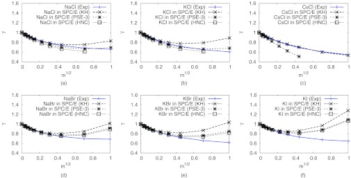
Mean activity coefficients of alkali halide salts in water. DRISM results were calculated with KH, PSE-3, and HNC closures and compared with experimental results.⁹⁶

The Debye-Hückel limiting law predicts almost correct behavior of activity coefficients at low concentrations. The Debye-Hückel constants of Eq. 11 were estimated from the slope at the zero concentration of the calculated activity coefficients (see Sec. II of the supplementary material).⁷⁶ Larger constants correspond to a more rapid decrease of the activity coefficients at low concentrations. The constants increased as the order of PSE-n closure increased. At 298 K, the estimated constant from Debye-Hückel theory is 1.1724 kg^1/2 mol^−1/2.⁷⁵ Ideally, the slope at the zero concentration calculated by DRISM should agree with the experiment. Consequently, the experimental Debye-Hückel constant also should match the calculated constants. Generally, the constants calculated by DRISM-KH agree with the experimental constant. The results of previous MD simulations⁶¹ suggest that the performance of the ion parameters of Joung and Cheatham⁵⁸ is good for mid-sized ions, such as Na⁺ and K⁺ for cations and Cl⁻ for anions. Consistent with MD, DRISM also achieves the best agreement with experimental mean activity coefficients for such mid-size ions. The experimental mean activity coefficients of NaCl and KCl at low concentrations were predicted best by PSE-3 closure, though there is dependency on LJ parameters of the ions and not all ion sizes give such good results (see Sec. III of the supplementary material).⁷⁶

The fact that the predicted results are similar to the experimental results at least shows that the average interaction between water and ion is well-preserved at low concentrations of the salts. If water-water interaction were too strong, the solvation free energy of ions would be more positive because water molecules would preferentially solvate other water molecules more than ions. If water-ion interaction were too strong, on the other hand, the solvation free energy of ions would be more negative for the same reason. It is, however, unclear whether accurate mean activity coefficients guarantee accurate activity coefficients for each ion. Separating the positive and negative ions in solution is not possible in practice and there is no experimental reference to compare with. Here, we have used MD simulation to estimate the activities of individual ions using classical pair-wise force fields, which share the potential energy equation with the RISM theory.

Fig. 2 shows the change of solvation free energies of the salts as a function of the salt concentration. The solvation free energies at the lowest concentrations of the MD results were estimated by Debye-Hückel theory. Both MD and RISM give a good account of the mean activity coefficients (Fig. 2a). However, the excess chemical potential of the cation estimated by MD simulations starts to increase around 0.04 m (Fig. 2b) but that of the anion keeps decreasing up to 0.5 m (Fig. 2c). Both curves estimated by DRISM were quite off from the curves of MD simulations, though the difference of the total excess chemical potential was quite similar even up to 0.1 m. The contributions from water and ions delicately determine the net excess chemical potentials of ions. The balance of the two contributions appears to be important but further investigation will be necessary for the deeper understanding of the discrepancy (see Sec. IV of the supplementary material).⁷⁶

Figure 2.

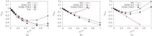
Change in excess chemical potential of NaCl as a function of salt concentration. Δμ_ex denotes the difference of the solvation free energy from that of zero concentration. Water models were SPC/E for MD calculation and cSPC/E for DRISM calculations. Total excess chemical potential difference (a) and differences for cation and anion ((b) and (c)) were plotted separately. The excess chemical potential of the lowest concentration of MD simulations were estimated by Debye-Hückel theory and the half of the total excess chemical potential was applied to the lowest concentration of each ion.

Absolute solvation free energies

In Sec. 4A, we discussed the relative solvation free energies of alkali-halide salts at various concentrations and compared the results of the DRISM with the results of MD simulations. In this section, we will discuss the absolute solvation free energies of the ions at infinite dilution. Comparing the excess chemical potentials of ions by DRISM-KH and DRISM-PSE3, it was found that the KH closure always produces a less negative excess chemical potential (Table 1). The total excess chemical potential was decomposed into electrostatic, μ_{ex, elec}, and vdW, μ_{ex, vdW}, contributions. μ_{ex, vdW} is the excess chemical potential with the charge of the ion set to zero. The electrostatic part is then the total excess chemical potential minus the vdW contribution,

$${\mu }_{\text{ex,elec}}={\mu }_{\text{ex}}-{\mu }_{\text{ex,vdW}}.$$

Both electrostatic and vdW contributions of PSE-3 were more negative than KH over the total space of LJ parameters (see Sec. V of the supplementary material).⁷⁶ The difference was most obvious in the electrostatic contribution where the PSE-3 closure renders the electrostatic contribution more negative as R_min and ɛ becomes smaller. That is, electrostatic differences increase as the ions become smaller and softer. The trend is opposite for the vdW contribution where the PSE-3 result is more negative as R_min and ε become larger. The net result is that for the most biologically common monovalent ions, Na⁺, K⁺, and Cl⁻, the difference between PSE-3 and KH is only about 1−1.5 kcal/mol (see also Table 1).

Table 1.

Decomposed absolute excess chemical potential of alkali- and halide ions in SPC/E (MD) or cSPC/E (DRISM) water. The experimental solvation free energies were determined on a scale where the free energy of hydration of the proton is taken to be −249.5 kcal/mol.

		MD58			DRISM-KH			DRISM-PSE3			DRISM-HNC
Ion	Exp97	Total	Elec	vdW	Total	Elec	vdW	Total	Elec	vdW	Total	Elec	vdW
Li+	−113.8	−113.3	−113.5	0.20	−108.30	−109.37	1.07	−111.16	−112.12	0.96	−111.42	−112.37	0.96
Na+	−88.7	−88.4	−88.9	0.48	−84.95	−87.51	2.56	−86.16	−88.47	2.31	−86.24	−88.54	2.30
K+	−71.2	−71.0	−71.8	0.81	−68.57	−73.01	4.45	−69.32	−73.27	3.95	−69.35	−73.30	3.94
Cl−	−89.1	−89.3	−96.0	6.6	−78.09	−93.57	15.48	−79.47	−93.74	14.27	−79.51	−93.75	14.24
Br−	−82.7	−82.7	−89.5	6.8	−72.20	−89.03	16.83	−73.67	−89.07	15.40	−73.72	−89.07	15.36
I−	−74.3	−74.4	−81.9	7.5	−62.65	−82.36	19.71	−64.41	−82.29	17.88	−64.46	−82.29	17.82

MD and experimental solvation free energies are similar because the LJ parameters were optimized for the target experimental values. The experimental solvation free energies listed in the table were rescaled assuming the solvation free energy of the proton is −249.5 kcal/mol. The number arguably excludes the “phase potential,”⁹⁸ which the free energy difference induced by transferring the solute from vacuum to the boundary of water. As both MD simulation and RISM have no solvent boundary, the calculated solvation free energies are expected to be close to the listed experimental numbers. Comparing DRISM-PSE-3 and MD simulations, it is found that the solvation free energies of DRISM-PSE-3 are more positive (Table 1). The values for cations are generally quite good, differing only by ∼2 kcal/mol but not so for anions, where is difference is ∼10 kcal/mol. To gain some insight about this behavior, μ_ex was decomposed into electrostatic and vdW contributions again. From this, it is apparent that the electrostatic contributions are generally quite good, with differences ranging from 0.3 to 2.3 kcal/mol and no obvious difference between anions and cations. The vdW contributions of PSE-3, however, are generally much more positive than MD simulations and the source of the discrepancy between cation and anion results. It is worth noting that while the DRISM vdW results are much larger for all ions, the values do increase with ion size as do the MD values. The effect of LJ parameters on the excess chemical potential varied depending on the closures (see Sec. V of the supplementary material).⁷⁶ Although the improvement is not as drastic as the electrostatic contribution, the vdW contributions of higher-order PSE closure deviates less from the MD simulations than do the KH results. Overall, we can conclude that higher-order PSE always agree better with MD simulations in terms of the absolute excess chemical potential.

Water activity

The absolute excess chemical potential of SPC/E water was calculated by DRISM and MD simulations. The experimental solvation free energy is known to be −6.31 kcal/mol.⁹⁹ It should be noted that the experimental number apparently includes the energy required in the gas phase to polarize the molecule to its solvated charge distribution, which is missing from the MD and DRISM models, based on fixed charge distributions.^{80, 100, 101} Comparing DRISM and MD results, it is observed that values decreased as the order PSE closure increased. However, even the HNC closure overestimates the excess chemical potential by 3.7 kcal/mol compared to MD calculations (see Sec. VI of the supplementary material).⁷⁶ As has been noted earlier,⁸¹ the electrostatic contributions are almost the same between MD and DRISM. In contrast to the case for ions, the electrostatic contribution for water is almost insensitive to the closure order of PSE, possibly because it is electrostatically neutral.

Experimentally, the excess chemical potential of water increases as the concentration of salt increases. However, the activity of water decreases because the ideal chemical potential decreases faster than the excess chemical potential of water increases (Figure 3). Water activity is extremely difficult to estimate directly from MD simulations because the dependency of the excess chemical potential of water activity on the concentration of electrolytes is very subtle. However, one can easily calculate the relative excess chemical potential of water using the DRISM theory in two different ways. The direct approach is to use Eq. 9 and compute μ_{ex, water} from the water distribution functions. Alternately, the Gibbs-Duhem equation, Eq. 24, relates the excess chemical potentials of water to that of the ions. If DRISM does not violate the thermodynamic consistency, the numbers from the two different expressions should be identical.

Figure 3.

The activity of water in NaCl solution and the corresponding osmotic coefficient (ϕ) calculated by DRISM-HNC. GD is the curve estimated by Gibbs-Duhem equation from the computed excess chemical potential of the ions ignoring the change of pressure (Eqs. 24, 25); the experimental values were also estimated by the equation from the experimental mean activity coefficients of the salt.⁹⁶

Because the density of MD simulations should be similar to the experimental results, the pressure estimated by the DRISM theory ideally should not be different from the experimental condition, 1 atm, at any concentration. If it is true, Eq. 24 can be used to estimate $\Delta {\mu }_{\text{ex,}w}^x$ (Fig. 3). If the Gibbs-Duhem equation was consistently obeyed by the DRISM theory, the results such as Fig. 3 would be equivalent to the results of Fig. 1. Since the mean activity coefficients of NaCl calculated by DRISM-HNC are close to experimental values (Fig. 1) at low concentrations, water activities are also reasonable, although deviations can be seen in Fig. 3 in the more sensitive osmotic coefficient.

In order to determine how well DRISM-HNC conforms to the Gibbs-Duhem relation, the excess chemical potential of water estimated by the theory ($\Delta {\mu }_{\text{ex,}w}^{\text{RISM}}$) can be compared to the excess chemical potential of water calculated via the Gibbs-Duhem equation using the excess chemical potentials of ions ($\Delta {\mu }_{\text{ex,}w}^{\text{GD}}$). As the change of the pressure of the system cannot be ignored and, in RISM calculations, the ideality of the system is defined by the ideal gas theory, the excess chemical potential should be calculated using Eq. 16 for $\Delta {\mu }_{\text{ex,}w}^{\text{GD}}$. The pressure-dependent term Δμ^press is numerically calculable if 1/ρ_w is known as a function of p, as shown in Eq. 18. When experimental liquid densities are used, values for Δμ^press, using the data listed in Sec. VII of the supplementary material,⁷⁶ are displayed in Table 2(a). It is worth noting that the DRISM pressures are much higher than 1 atm and the pressure increases with salt concentration. The increment is not trivial and thus Δμ^press becomes the dominant part of $\Delta {\mu }_{\text{ex,}w}^{\text{GD}}$. $\Delta {\mu }_{\text{ex,}w}^{\text{GD}}$ and $\Delta {\mu }_{\text{ex,}w}^{\text{RISM}}$ agreed well up to a few milli-molal concentration but increasingly differ as concentration increases (Fig. 4). Although the Gibbs-Duhem relation is not strictly obeyed, the two estimates differ by less than 0.03 kcal/mol, and we conclude that Gibbs-Duhem relation is qualitatively observed.

Table 2.

Excess chemical potential (in cal/mol) of water in NaCl solution calculated directly and via the Gibbs-Duhem equation. $\Delta {\mu }_{\text{ex,}w}^{\text{GD}}=\Delta {\mu }_{\text{ex,}w}^{\text{sol}}+\Delta {\mu }^{\text{press}}+\Delta {\mu }^{\rho }$ (Eqs. 16, 17, 18, 19) was calculated from the excess chemical potential of ions via Gibbs-Duhem equation and $\Delta {\mu }_{\text{ex,}w}^{\text{RISM}}$ was directly calculated using Eq. 9 in the main text. Data were collected using experimental solution density (a) and constant molar density of the solution (b).

m	$\Delta {\mu }_{\text{ex,}w}^{\text{sol}}$	Δμpress	Δμρ	$\Delta {\mu }_{\text{ex,}w}^{\text{GD}}$	$\Delta {\mu }_{\text{ex,}w}^{\text{RISM}}$
(a)
0	0.0000	0.0	0.0000	0.0	0.0
0.001	0.0004	0.2	−0.0115	0.2	0.3
0.002	0.0008	0.4	−0.0229	0.4	0.6
0.005	0.0032	1.1	−0.0573	1.0	1.5
0.01	0.0085	2.2	−0.1142	2.1	3.0
0.02	0.0233	4.5	−0.2266	4.3	5.9
0.05	0.0818	11.7	−0.5643	11.3	14.9
0.1	0.2008	24.3	−1.1192	23.3	29.8
0.2	0.4441	50.3	−2.2114	48.6	59.4
0.5	1.0121	133.4	−5.4030	129.0	147.9
(b)
0	0.0000	0.0	0.0000	0.0	0.0
0.001	0.0004	−0.1	0.0000	−0.1	0.0
0.002	0.0009	−0.2	0.0000	−0.2	−0.1
0.005	0.0033	−0.4	0.0000	−0.4	−0.1
0.01	0.0091	−0.8	0.0000	−0.7	−0.2
0.02	0.0256	−1.4	0.0000	−1.4	−0.4
0.05	0.0963	−3.0	0.0001	−2.9	−1.0
0.1	0.2582	−5.0	0.0002	−4.7	−1.8
0.2	0.6708	−7.7	0.0006	−7.0	−3.1
0.5	2.3976	−9.9	0.0012	−7.5	−5.7

Figure 4.

Comparison of Δμ_{ex, w} calculated from the excess chemical potential of ions via Gibbs-Duhem equation and calculated using Eq. 9. The solid lines and dotted lines indicate the data from experimental solution density and constant molar density, respectively.

The pressure is closely linked to the density of the molecules in the system. On that account, we tried the same calculation with a different density set. Instead of using the experimental solution density, the total molar concentration was preserved. That is, ρ_w is adjusted to keep ρ_w + ∑_iρ_i constant regardless of the concentration of the salt. In this case, we observed that the system pressure decreases as the concentration of NaCl increases, although the absolute pressure still stays high. The Gibbs-Duhem relationship was tested with the modified system and the results are listed in Table 2(b). Due to the decrement of the pressure, Δμ^press also decreases. The absolute contribution of Δμ^press to the excess chemical potential of water has decreased but it is still dominant. $\Delta {\mu }_{\text{ex,}w}^{\text{GD}}$ and $\Delta {\mu }_{\text{ex,}w}^{\text{RISM}}$ also semi-quantitatively agreed and we also could not observe serious violation of Gibbs-Duhem relation. While DRISM-PSE-n does not strictly obey the Gibbs-Duhem as XRISM-PSE-n does, the agreement is close.

Radial distribution functions

Comparisons of the radial distributions of DRISM and MD simulations provide insight into the differences in solvent structure predicted by the two methods. Fig. 5 shows the radial distributions of NaCl solutions at 0.6688 m concentration, with first shell coordination numbers reported in Table 3 and Sec. IX of the supplementary material.⁷⁶ The experimental radial distributions are also shown for reference. We also calculated radial distribution functions at two other concentrations: 0.3469 m and 1.3877 m (see Sec. VIII of the supplementary material).⁷⁶ The following discussions apply to all concentrations in this range. The radial distribution of Na-O from DRISM had the correct position for the first and second peaks compared to the MD simulation (Fig. 5a), but the height of the peaks are lower than MD. This low peak results in nearly one missing oxygen from the first solvation shell. Higher order PSE-n closures narrow the error in the first peak height, but with only a very small impact on the coordination number. The radial distribution of Na-H is also fairly accurate in predicting the correct position of the first 3 peaks. Although it is not as good as g_Na-O, higher order PSE-n also slightly improved the height of the first peak. The low height of the first peak is compensated by its broadness, giving a coordination number close the MD value of 14.9, though with a strong closure dependence. This indicates that the water structure around Na⁺ is qualitatively close to that from MD simulations and from experiment.

Figure 5.

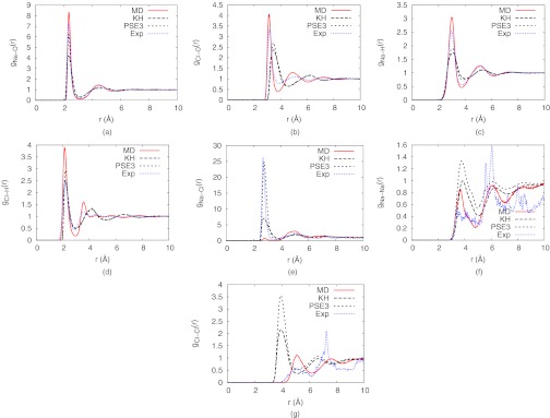
Radial distribution functions of NaCl solutions at the concentration of 0.6688 m calculated with DRISM-KH, DRISM-PSE3, and MD simulation and compared against experimental radial distributions.¹⁰², ¹⁰³

Table 3.

Coordination numbers for Na⁺ and Cl⁻ at 0.6688 m from DRISM and MD simulations. Experimental data (the last column) include the error range in the parenthesis.

	DRISM-PSE-3	DRISM-KH	MD	Mancinelli et al.102
Na+−O	4.85	4.98	5.79	5.3 (0.8)
Na+−H	14.5	15.7	14.8	13.9 (1.0)
Na+−Na+	0.132	0.100	0.060	…
Na+−Cl−	0.394	0.211	0.012	…
Cl−−O	11.8	12.5	7.07	6.9 (1.0)
Cl−−H	5.90	6.13	6.81	6.0 (1.1)
Cl−−Cl−	0.240	0.170	0.171	…

On the other hand, g_Cl-O from DRISM is quite different from the MD simulation (Fig. 5b). The first several peaks are pushed farther away in DRISM, and the first peak is broader, which implies that the second water shell is partially collapsed into the first peak. This is reflected in a 76% increase in the Cl⁻−O coordination number of DRISM-PSE-3 compared to MD, and is similar to the collapse of the O−O second solvation shell in water.⁸¹ The two hydrogens of the water in the first shell are sharper in the MD simulation (Fig. 5d) but the extra oxygens in the DRISM first shell do not contribute any extra hydrogens to the coordination number. In fact, there is a slight decrease in the first hydrogen shell relative to MD. The displaced, broadened first oxygen peak also appears to shift the DRISM second peak of the hydrogen, which is believed to be the other hydrogen atom of the water molecules in the first shell, farther (∼4.2 Å) and broaden it as well. As opposed to the observation, the second peak appears at ∼3.5 Å for the MD simulation and experiment. Qualitatively, the DRISM water structure around anions is less defined than MD with weaker binding. This is consistent with results for the excess chemical potential of water where DRISM gave values ∼10 kcal/mol higher than MD.

While the first peaks of the radial distribution function between ions and water sites calculated by DRISM were lower than MD results, the first peaks of the radial distribution of ion-ion pairs are always higher than MD simulations (Figs. 5e, 5f, 5g). Contact ion pairs of cation and anion association (which the first peak of g_Na-Cl indicate) is the most extreme example with DRISM-PSE-3 predicting a coordination number more than 30 times that of MD. Interestingly, the first peak of the DRISM is closer to the experimental results than the MD simulation. Among the three ion-ion radial distributions, g_Cl-Cl is substantially distorted (Fig. 5g), which may be due to the fewer ordered water molecules around Cl⁻. In particular, the contact pair of Cl−Cl is much closer and higher peaked than in the MD simulation. We presume that, at least in part, the extremely high pressure makes the pair more compact. Along with the pressure, the bigger angle of Cl−H−O appears to distort water structures around the anion extensively. Unlike the counterpart angle of the cation (Na−O−H), Cl−H−O could be more sensitive to the structure of the second water shell. However, the same effect was not observed for Na−Na pair (Fig. 5f). Anions generally have larger R_min than cations and the difference of the softness of the two ions might also explain the different behavior. g_Na-Na of the DRISM is quite accurate at predicting the radii of the peaks though they are still too high and broad. It is in accord with relatively accurate water structure around Na⁺.

CONCLUSIONS

The properties of aqueous ionic solutions are important topics of basic physical chemistry, but are also essential to the description of the environment of biological macromolecules. The RISM methodology is attractive due to its ability to rapidly calculate equilibrium properties over a wide range of concentrations and provide semi-quantitative results. A common unknown in any study involving the RISM treatment of ionic solutions is the accuracy of the RISM picture for a given potential energy function. To this end, we have characterized the DRISM solution of Joung-Cheatham⁵⁸ SPC/E monovalent ion force field with the PSE-n family of closures and compared our results directly against both MD results for the same models and the desired empirical properties.

The Joung-Cheatham⁵⁸ SPC/E parameter set for monovalent ions is an important benchmark given its excellent reproduction of bulk solution properties and widespread use.^{58, 59, 60, 61} Generally, DRISM was able to capture the behavior of this parameter set, accurately reproducing mean ion activity coefficients and solvent polarization free energies. However, several shortcomings are apparent. The non-polar contribution to solvation free energy is drastically different than that calculated from MD, particularly for larger ions. Another artifact is the extremely high pressure, several thousand atmospheres, calculated by DRISM. This is consistent with the observed non-polar solvation free energy; the chemical potential of an uncharged solute should be higher in a high-pressure solution than a low-pressure one. It is also consistent with the RDFs produced by XRISM and DRISM for pure water and DRISM for salt solutions, which have the general characteristics observed in experiment for these liquids under high pressure.^{104, 105, 106}

Closure approximations, required for the solution of the RISM and all OZ-like equations, are a major factor in determining the success or failure of a calculation. HNC and, more recently, KH closures have been popular choices for their simplicity, success with ionic solutions and having an exact, closed-form expression for the excess chemical potential, free energy, and pressure. HNC's greatest success has been with primitive models of aqueous ionic solutions where water is replaced with a dielectric constant and the ions form a dilute gas^{107, 108, 109, 110, 111, 112, 113} or the effective potentials between ions include the aqueous environment.¹¹⁴ When molecular water is introduced, the system enters the high density regime, where HNC has long been known to grossly overestimate pressures and excess chemical potentials,^{55, 115} as we have observed here. KH has found popularity as it converges quickly, and is numerically robust, with solutions for many systems where HNC fails. However, our results show that KH dampens attractive interactions while further exacerbating overly positive excess chemical potentials and pressures. The PSE-n closure interpolates between KH and HNC and PSE-3, in particular, provides a useful compromise between the two established closures. It allows relatively rapid and efficient convergence, especially when bootstrapping from PSE-1 and -2 solutions, provides RDFs similar to those of HNC and has an exact, closed-form expression for the excess chemical potential, free energy, and pressure. Unfortunately, it also suffers from the same deficits of excessive pressure and excess chemical potentials and does not greatly change the fundamental picture of aqueous ionic solutions in DRISM.

The dielectric consistency of DRISM is an essential feature of the theory, but appears to come at the cost of thermodynamic consistency. While the HNC family of closures is known to have inconsistencies between the compressibility and free energy routes to the pressure, the Gibbs-Duhem relation should hold for XRISM when using only the free energy based expression. For DRISM, the Gibbs-Duhem relation fails, though not badly: differences in Fig. 4 are much less that kT.

Even with its shortcomings, the flexibility, speed, and semi-quantitative accuracy make DRISM a valuable tool to the study of aqueous ionic solutions and to use with 3D-RISM for complex solutes. The most rigorous path to improving DRISM is through modifying the closure, but empirical corrections for errors in non-polar solvation show much practical promise.^{71, 73, 116} In particular, the expression for the excess chemical potential for PSE-n closures gives useful and reliable results for many properties of interest for aqueous electrolytes.

APPENDIX A: LONG-RANGE COULOMB INTERACTIONS

Periodic boundary conditions, combined with Ewald summation,¹¹⁷ is one of the popular ways to treat long-ranged electrostatic potential in MD simulations. In the RISM theory, long-ranged (i.e., Coulomb) interactions are problematic when calculating the Fourier transform required to perform the convolution integrals in Eqs. 2, 6, and are handled by taking advantage of the long-ranged behavior of the correlation functions.¹⁹, ²⁰, ⁵³, ¹¹⁸, ¹¹⁹, ¹²⁰, ¹²¹, ¹²² At long-range, the direct correlation function asymptotically approaches −βu¹¹⁸

$$\begin{array}{cc}\hfill c_{\alpha \gamma }^{\text{(lr)}}\left(r\right)=& -\beta u_{\alpha \gamma }^{\left(\text{lr}\right)}\left(r\right)=-\frac{1}{k_{B}T}\frac{q_{\alpha }{q}_{\gamma }}{r}\text{erf}\left(\frac{r}{\eta }\right),\hfill \end{array}$$ (A1)

$$\begin{array}{cc}\hfill c_{\alpha \gamma }^{\text{(lr)}}\left(k\right)=& -\frac{4\pi }{k_{B}T}\frac{q_{\alpha }{q}_{\gamma }}{k^2}\exp \left(-\frac{k^2{\eta }^2}{4}\right).\hfill \end{array}$$ (A2)

Before transforming from real to reciprocal-space, the long-range component is subtracted off and then restored in reciprocal-space.

The same problem exists, to a lesser extent, for transforming h back to real-space after the convolution is complete. The asymptotic form of h can be obtained with the combination of Eq. 2 and one of the equations above, but the form is not amenable to being analytically Fourier transformed.¹²³ In practice, a simplified form is sufficient.

$$\begin{array}{cc}\hfill h_{\alpha \gamma }^{\text{(lr)}}\left(r\right)=& -\frac{1}{2\varepsilon k_{B}T}\frac{Q_{\alpha }{Q}_{\gamma }}{r}\exp \left(\frac{{\kappa }_{\text{D}}^2{\eta }^2}{4}\right)\hfill \\ & \times \left[\exp \left(-{\kappa }_{\text{D}}r\right)\text{erfc}\left(\frac{{\kappa }_{\text{D}}\eta }{2}-\frac{r}{\eta }\right)\right.\hfill \\ & \left.-\exp \left({\kappa }_{\text{D}}r\right)\text{erfc}\left(\frac{{\kappa }_{\text{D}}\eta }{2}+\frac{r}{\eta }\right)\right],\hfill \end{array}$$ (A3)

$$\begin{array}{cc}\hfill h_{\alpha \gamma }^{\text{(lr)}}\left(k\right)=& -\frac{4\pi }{\varepsilon k_{B}T}\frac{Q_{\alpha }{Q}_{\gamma }}{k^2+{\kappa }_{\text{D}}^2}\exp \left(-\frac{k^2{\eta }^2}{4}\right),\hfill \end{array}$$ (A4)

where ${\kappa }_{\text{D}}={\sum }_{\lambda }\sqrt{4\pi \beta {\rho }_{\lambda }{Q}_{\lambda }^2/\varepsilon }$ is the contribution to the inverse Debye length. Note that Q_α is the total charge of molecular species to which α belongs.

APPENDIX B: IDEAL AND EXCESS CHEMICAL POTENTIALS

The chemical potential of solute, i can be divided into the “ideal” part and the “excess” part:

$${\mu }_i=k_{B}T\ln {\rho }_i{\Lambda }^3+{\mu }_{\text{ex},i},$$ (B1)

where Λ is the de Broglie wavelength. The ideal part above is derived from the ideal gas theory. In practical work, especially dealing with solutions, this division is defined differently depending on the unit of concentration used:

$${\mu }_i={\mu }_c^{*}+k_{B}T\ln (c_i/c^{\circ })+{\mu }_{\text{ex},i}^c,$$ (B2)

$${\mu }_i={\mu }_x^{*}+k_{B}T\ln x_i+{\mu }_{\text{ex},i}^x,$$ (B3)

$${\mu }_i={\mu }_m^{*}+k_{B}T\ln (m_i/m^{\circ })+{\mu }_{\text{ex},i}^m.$$ (B4)

Here c, x, and m denote molar concentration, mole fraction, and molal concentration. c° and m° represent the unit standard concentrations, which are 1 mol/L and 1 mol/kg × solvent. Asterisks indicate reference states. Each equation above defines a slightly different excess chemical potential of the solution. ${\mu }_{\text{ex},i}^c$ can be expressed using Eqs. B1, B2,

$$\begin{array}{cc}\hfill {\mu }_{\text{ex},i}^c& =k_{B}T\ln {\Lambda }^3-{\mu }_c^{*}+k_{B}T\ln ({\rho }_i{c}^{\circ }/c_i)+{\mu }_{ex,i}\hfill \\ & =k_{B}T\ln {\Lambda }^3-{\mu }_c^{*}+k_{B}T\ln \left(N_A{c}^{\circ }\right)+{\mu }_{ex,i},\hfill \end{array}$$

where N_A is the Avogadro's number. The first three terms are independent of the concentration of the solute. Therefore, the difference of the excess chemical potential of the solution at any two different concentrations is same as the difference of the excess chemical potentials,

$$\Delta {\mu }_{\text{ex},i}^c={\mu }_{\text{ex},i}-{\mu }_{\text{ex},\infty }=\Delta {\mu }_{\text{ex},i}.$$

In the same manner, ${\mu }_{\text{ex},i}^x$ and ${\mu }_{\text{ex},i}^m$ also can be expressed in term of the excess chemical potential using Eqs. B3, B4, B1. For ${\mu }_{\text{ex},i}^x$,

$$\begin{array}{cc}\hfill {\mu }_{\text{ex},i}^x& =k_{B}T\ln {\Lambda }^3-{\mu }_x^{*}+k_{B}T\ln (\rho /x)+{\mu }_{\mathrm{ex},i}.\hfill \end{array}$$ (B5)

At the infinitely dilute solution,

$$\begin{array}{cc}\hfill 0& =k_{B}T\ln {\Lambda }^3-{\mu }_x^{*}+k_{B}T\ln ({\rho }_{\infty }/x_{\infty })+{\mu }_{\mathrm{ex},\infty }.\hfill \end{array}$$ (B6)

If Eq. B6 is subtracted from Eq. B5,

$$\begin{array}{cc}\hfill \Delta {\mu }_{\text{ex},i}^x& =k_{B}T\ln \left(\frac{{\sum }_j{\rho }_j}{{\sum }_j{\rho }_{j,\infty }}\right)+\Delta {\mu }_{\text{ex},i}.\hfill \end{array}$$ (B7)

Inside the logarithm, there remains the ratio of the summation of the number densities of all the species in the solution at the two conditions. For ${\mu }_{\text{ex},i}^m$,

$$\begin{array}{cc}\hfill {\mu }_{\text{ex},i}^m& =k_{B}T\ln {\Lambda }^3-{\mu }_m^{*}+k_{B}T\ln ({\rho }_i{m}^{\circ }/m_i)+{\mu }_{\mathrm{ex},i}.\hfill \end{array}$$ (B8)

In the infinitely dilute solution,

$$\begin{array}{cc}\hfill 0& =k_{B}T\ln {\Lambda }^3-{\mu }_m^{*}+k_{B}T\ln ({\rho }_{\infty }{m}^{\circ }/m_{i,\infty })+{\mu }_{\mathrm{ex},\infty }.\hfill \end{array}$$ (B9)

Subtracting Eq. B9 from Eq. B8 yields

$$\begin{array}{cc}\hfill \Delta {\mu }_{\text{ex},i}^m& =k_{B}T\ln ({\rho }_w/{\rho }_{w,\infty })+\Delta {\mu }_{\mathrm{ex},i},\hfill \end{array}$$

where the subindex w denotes the solvent. This agrees with Eq. 10.

References

- Still W. C., Tempczyk A., Hawley R. C., and Hendrickson T., “Semianalytical treatment of solvation for molecular mechanics and dynamics,” J. Am. Chem. Soc. 112(16), 6127–6129 (1990). 10.1021/ja00172a038 [DOI] [Google Scholar]
- Bashford D. and Case D. A., “Generalized Born models of macromolecular solvation effects,” Annu. Rev. Phys. Chem. 51(1), 129–152 (2000). 10.1146/annurev.physchem.51.1.129 [DOI] [PubMed] [Google Scholar]
- Tsui V. and David A., “Molecular dynamics simulations of nucleic acids with a generalized Born solvation model,” J. Am. Chem. Soc. 122(11), 2489–2498 (2000). 10.1021/ja9939385 [DOI] [Google Scholar]
- Honig B. and Nicholls A., “Classical electrostatics in biology and chemistry,” Science 268, 1144–1149 (1995). 10.1126/science.7761829 [DOI] [PubMed] [Google Scholar]
- Sharp K. A. and Honig B., “Calculating total electrostatic energies with the nonlinear Poisson-Boltzmann equation,” J. Phys. Chem. 94, 7684–7692 (1990). 10.1021/j100382a068 [DOI] [Google Scholar]
- Baker N. A., Bashford D., and Case D. A., “Implicit solvent electrostatics in biomolecular simulation,” in New Algorithms for Macromolecular Simulation, edited by Leimkuhler B., Chipot C., Elber R., Laaksonen A., Mark A., Schlick T., Schuette C., and Skeel R. (Springer-Verlag, 2006), pp. 263–295. [Google Scholar]
- Ornstein L. S. and Zernike F., “Accidental deviations of density and opalescence at the critical point of a single substance,” Proc. R. Acad. Sci. Amsterdam 17, 793 (1914). [Google Scholar]
- Ornstein L. S. and Zernike F., “Accidental deviations of density and opalescence at the critical point of a single substance,” in The Equilibrium Theory of Classical Fluids: A Lecture Note and Reprint Volume (W. A. Benjamin, 1964), pp. III–2–16. [Google Scholar]
- Hansen J.-P. and McDonald I. R., Theory of Simple Liquids, 2nd ed. (Academic, London, Great Britain, 1990), Chap. 5, pp. 97–144. [Google Scholar]
- Chandler D. and Andersen H. C., “Optimized cluster expansions for classical fluids. II. Theory of molecular liquids,” J. Chem. Phys. 57, 1930–1937 (1972). 10.1063/1.1678513 [DOI] [Google Scholar]
- Hirata F. and Rossky P. J., “An extended RISM equation for molecular polar fluids,” Chem. Phys. Lett. 83(2), 329–334 (1981). 10.1016/0009-2614(81)85474-7 [DOI] [Google Scholar]
- Perkyns J. S. and Pettitt B. M., “A dielectrically consistent interaction site theory for solvent-electrolyte mixtures,” Chem. Phys. Lett. 190(6), 626–630 (1992). 10.1016/0009-2614(92)85201-K [DOI] [Google Scholar]
- Bruzzone S., Malvaldi M., and Chiappe C., “A RISM approach to the liquid structure and solvation properties of ionic liquids,” Phys. Chem. Chem. Phys. 9, 5576 (2007). 10.1039/b708530c [DOI] [PubMed] [Google Scholar]
- Bruzzone S., Malvaldi M., and Chiappe C., “Solvation thermodynamics of alkali and halide ions in ionic liquids through integral equations,” J. Chem. Phys. 129, 074509 (2008). 10.1063/1.2970931 [DOI] [PubMed] [Google Scholar]
- Fedotova M. V., Kruchinin S. E., Rahman H. M. A., and Buchner R., “Features of ion hydration and association in aqueous rubidium fluoride solutions at ambient conditions,” J. Mol. Liq. 159(1), 9–17 (2011). 10.1016/j.molliq.2010.04.009 [DOI] [Google Scholar]
- Stoyanov S. R., Gusarov S., and Kovalenko A., “Multiscale modelling of asphaltene disaggregation,” Mol. Simul. 34(10–15), 953–960 (2008). 10.1080/08927020802411711 [DOI] [Google Scholar]
- Beglov D. and Roux B., “An integral equation to describe the solvation of polar molecules in liquid water,” J. Phys. Chem. B 101(39), 7821–7826 (1997). 10.1021/jp971083h [DOI] [Google Scholar]
- Kovalenko A. and Hirata F., “Three-dimensional density profiles of water in contact with a solute of arbitrary shape: A RISM approach,” Chem. Phys. Lett. 290(1–3), 237–244 (1998). 10.1016/S0009-2614(98)00471-0 [DOI] [Google Scholar]
- Kovalenko A. and Hirata F., “Self-consistent description of a metal-water interface by the Kohn-Sham density functional theory and the three-dimensional reference interaction site model,” J. Chem. Phys. 110, 10095 (1999). 10.1063/1.478883 [DOI] [Google Scholar]
- Kovalenko A., “Three-dimensional RISM theory for molecular liquids and solid-liquid interfaces,” in Molecular Theory of Solvation, edited by Hirata F. (Kluwer Academic, 2003), Chap. 4, pp. 169–276. [Google Scholar]
- Maruyama Y., Yoshida N., and Hirata F., “Electrolytes in biomolecular systems studied with the 3d-rism/rism theory,” Interdiscip. Sci. 3(4), 290–307 (2011). 10.1007/s12539-011-0104-7 [DOI] [PubMed] [Google Scholar]
- Howard J. J. and Pettitt B. M., “Integral equations in the study of polar and ionic interaction site fluids,” J. Stat. Phys. 145, 441–466 (2011). 10.1007/s10955-011-0260-5 [DOI] [PMC free article] [PubMed] [Google Scholar]
- Luchko T., Joung I. S., and Case D. A., “Integral equation theory of biomolecules and electrolytes,” in Innovations in Biomolecular Modeling and Simulations, RSC Biomolecular Sciences Vol. 1 (Royal Society of Chemistry, 2012), Chap. 4, pp. 51–86. [Google Scholar]
- Pettitt B. M. and Rossky P. J., “Integral equation predictions of liquid state structure for waterlike intermolecular potentials,” J. Chem. Phys. 77(3), 1451–1457 (1982). 10.1063/1.443972 [DOI] [Google Scholar]
- Hirata F., Pettitt B. M., and Rossky P. J., “Application of an extended RISM equation to dipolar and quadrupolar fluids,” J. Chem. Phys. 77, 509 (1982). 10.1063/1.443606 [DOI] [Google Scholar]
- Hirata F., Rossky P. J., and Pettitt B. M., “The interionic potential of mean force in a molecular polar solvent from an extended RISM equation,” J. Chem. Phys. 78, 4133 (1983). 10.1063/1.445090 [DOI] [Google Scholar]
- Pettitt B. M. and Rossky P. J., “Alkali halides in water: Ion-solvent correlations and ion-ion potentials of mean force at infinite dilution,” J. Chem. Phys. 84, 5836 (1986). 10.1063/1.449894 [DOI] [Google Scholar]
- Chandler D., “The dielectric constant and related equilibrium properties of molecular fluids: Interaction site cluster theory analysis,” J. Chem. Phys. 67, 1113 (1977). 10.1063/1.434962 [DOI] [Google Scholar]
- Cummings P. T. and Stell G., “Exact asymptotic form of the site-site direct correlation function for rigid polar molecules,” Mol. Phys. 44(2), 529–531 (1981). 10.1080/00268978100102621 [DOI] [Google Scholar]
- Perkyns J. and Pettitt B. M., “Integral-equation approaches to structure and thermodynamics of aqueous salt-solutions,” Biophys. Chem. 51(2–3), 129–146 (1994). 10.1016/0301-4622(94)00056-5 [DOI] [PubMed] [Google Scholar]
- Perkyns J. S. and Pettitt B. M., “A site-site theory for finite concentration saline solutions,” J. Chem. Phys. 97(10), 7656–7666 (1992). 10.1063/1.463485 [DOI] [Google Scholar]
- Imai T., Nomura H., Kinoshita M., and Hirata F., “Partial molar volume and compressibility of alkali-halide ions in aqueous solution: Hydration shell analysis with an integral equation theory of molecular liquids,” J. Phys. Chem. B 106(29), 7308–7314 (2002). 10.1021/jp014504a [DOI] [Google Scholar]
- Yu H. A., Roux B., and Karplus M., “Solvation thermodynamics: An approach from analytic temperature derivatives,” J. Chem. Phys. 92, 5020 (1990). 10.1063/1.458538 [DOI] [Google Scholar]
- Yu H. A. and Karplus M., “A thermodynamic analysis of solvation,” J. Chem. Phys. 89, 2366 (1988). 10.1063/1.455080 [DOI] [Google Scholar]
- Morita T., “Theory of classical fluids: Hyper-netted chain approximation, I (formulation for a one-component system),” Prog. Theor. Phys. 20, 920 (1958). 10.1143/PTP.20.920 [DOI] [Google Scholar]
- Yoshida N., Phongphanphanee S., and Hirata F., “Selective ion binding by protein probed with the statistical mechanical integral equation theory,” J. Phys. Chem. B 111(17), 4588–95 (2007). 10.1021/jp0685535 [DOI] [PubMed] [Google Scholar]
- Schmeer G. and Maurer A., “Development of thermodynamic properties of electrolyte solutions with the help of RISM-calculations at the Born-Oppenheimer level,” Phys. Chem. Chem. Phys. 12(10), 2407–2417 (2010). 10.1039/b917653e [DOI] [PubMed] [Google Scholar]
- Kast S. M. and Kloss T., “Closed-form expressions of the chemical potential for integral equation closures with certain bridge functions,” J. Chem. Phys. 129(23), 236101 (2008). 10.1063/1.3041709 [DOI] [PubMed] [Google Scholar]
- Raineri F. O. and Stell G., “Dielectrically nontrivial closures for the RISM integral equation,” J. Phys. Chem. B 105(47), 11880–11892 (2001). 10.1021/jp0121163 [DOI] [Google Scholar]
- González-Mozuelos P., “A simple phenomenological fix for the dielectric constant within the reference interaction site model approach,” J. Phys. Chem. B 110(45), 22702–22711 (2006). 10.1021/jp0645869 [DOI] [PubMed] [Google Scholar]
- Chong S. H. and Hirata F., “Ion hydration: Thermodynamic and structural analysis with an integral equation theory of liquids,” J. Phys. Chem. B 101(16), 3209–3220 (1997). 10.1021/jp9608786 [DOI] [Google Scholar]
- Chuev G., Chiodo S., Erofeeva S., Fedorov M., Russo N., and Sicilia E., “A quasilinear RISM approach for the computation of solvation free energy of ionic species,” Chem. Phys. Lett. 418, 485 (2006). 10.1016/j.cplett.2005.10.117 [DOI] [Google Scholar]
- Chiodo S., Chuev G. N., Erofeeva S. E., Fedorov M. V., Russo N., and Sicilia E., “Comparative study of electrostatic solvent response by RISM and PCM methods,” Int. J. Quantum Chem. 107, 265 (2007). 10.1002/qua.21188 [DOI] [Google Scholar]
- Fedorov M. V. and Kornyshev A. A., “Unravelling the solvent response to neutral and charged solutes,” Mol. Phys. 105, 1 (2007). 10.1080/00268970601110316 [DOI] [Google Scholar]
- Chuev G. N., Fedorov M. V., Chiodo S., Russo N., and Sicilia E., “Hydration of ionic species studied by the reference interaction site model with a repulsive bridge correction,” J. Comput. Chem. 29(14), 2406–2415 (2008). 10.1002/jcc.20979 [DOI] [PubMed] [Google Scholar]
- Yamazaki T., Kovalenko A., Murashov V. V., and Patey G. N., “Ion solvation in a water-urea mixture,” J. Phys. Chem. B 114(1), 613–619 (2010). 10.1021/jp908814t [DOI] [PubMed] [Google Scholar]
- Hummer G. and Soumpasis D., “An extended RISM study of simple electrolytes: Pair correlations in a NaCl-SPC water model,” Mol. Phys. 75, 633 (1992). 10.1080/00268979200100461 [DOI] [Google Scholar]
- Hummer G., Soumpasis D. M., and Neumann M., “Pair correlations in an NaCl-SPC water model,” Mol. Phys. 77, 769 (1992). 10.1080/00268979200102751 [DOI] [Google Scholar]
- Perkyns J. and Pettitt B. M., “On the solubility of aqueous electrolytes,” J. Phys. Chem. 98(19), 5147–5151 (1994). 10.1021/j100070a034 [DOI] [Google Scholar]
- Kinoshita M. and Hirata F., “Analysis of salt effects on solubility of noble gases in water using the reference interaction site model theory,” J. Chem. Phys. 106(12), 5202–5215 (1997). 10.1063/1.473519 [DOI] [Google Scholar]
- Fedotova M. V., Oparin R. D., and Trostin V. N., “Structure formation of aqueous electrolyte solutions under extreme conditions by the extended RISM-approach. A possibility of predicting,” J. Mol. Liq. 91(1–3), 123–133 (2001). 10.1016/S0167-7322(01)00154-4 [DOI] [Google Scholar]
- Fedotova M. V., “Effect of temperature and pressure on structural self-organization of aqueous sodium chloride solutions,” J. Mol. Liq. 153(1), 9–14 (2010). 10.1016/j.molliq.2009.05.006 [DOI] [Google Scholar]
- Kovalenko A. and Hirata F., “Potentials of mean force of simple ions in ambient aqueous solution. I. Three-dimensional reference interaction site model approach,” J. Chem. Phys. 112(23), 10391–10402 (2000). 10.1063/1.481676 [DOI] [Google Scholar]
- Rushbrooke G. S. and Hutchinson P., “On the internal consistency of the hyper-chain approximation in the theory of classical fluids,” Physica 27, 647 (1961). 10.1016/0031-8914(61)90009-X [DOI] [Google Scholar]
- Verlet L. and Levesque D., “On the theory of classical fluids II,” Physica 28, 1124–1142 (1962). 10.1016/0031-8914(62)90058-7 [DOI] [Google Scholar]
- Stell G., “Self-consistent equations for the radial distribution function,” Mol. Phys. 16, 209 (1969). 10.1080/00268976900100271 [DOI] [Google Scholar]
- Santos A., Fantoni R., and Giacometti A., “Thermodynamic consistency of energy and virial routes: An exact proof within the linearized Debye-Hückel theory,” J. Chem. Phys. 131(18), 181105 (2009). 10.1063/1.3265991 [DOI] [PubMed] [Google Scholar]
- Joung I. S. and T. E.CheathamIII, “Determination of alkali and halide monovalent ion parameters for use in explicitly solvated biomolecular simulations,” J. Phys. Chem. B 112, 9020–9041 (2008). 10.1021/jp8001614 [DOI] [PMC free article] [PubMed] [Google Scholar]
- Aragones J. L., Sanz E., and Vega C., “Solubility of NaCl in water by molecular simulation revisited,” J. Chem. Phys. 136(24), 244508 (2012). 10.1063/1.4728163 [DOI] [PubMed] [Google Scholar]
- Moučka F., Lísal M., and Smith W. R., “Molecular simulation of aqueous electrolyte solubility. 3. Alkali-halide salts and their mixtures in water and in hydrochloric acid,” J. Phys. Chem. B 116(18), 5468–78 (2012). 10.1021/jp301447z [DOI] [PubMed] [Google Scholar]
- Joung I. S. and T. E.CheathamIII, “Molecular dynamics simulations of the dynamic and energetic properties of alkali and halide ions using water-model-specific ion parameters,” J. Phys. Chem. B 113(40), 13279–13290 (2009). 10.1021/jp902584c [DOI] [PMC free article] [PubMed] [Google Scholar]
- Urbič T., Vlachy V., Kalyuzhnyi Y. V., and Dill K. A., “Orientation-dependent integral equation theory for a two-dimensional model of water,” J. Chem. Phys. 118, 5516 (2003). 10.1063/1.1556754 [DOI] [Google Scholar]
- Sumi T. and Sekino H., “An interaction site model integral equation study of molecular fluids explicitly considering the molecular orientation,” J. Chem. Phys. 125, 034509 (2006). 10.1063/1.2215603 [DOI] [PubMed] [Google Scholar]
- Kovalenko A. and Hirata F., “Hydration free energy of hydrophobic solutes studied by a reference interaction site model with a repulsive bridge correction and a thermodynamic perturbation method,” J. Chem. Phys. 113(7), 2793–2805 (2000). 10.1063/1.1305885 [DOI] [Google Scholar]
- Hirata F., “Theory of molecular liquids,” in Molecular Theory of Solvation, edited by Hirata F. (Kluwer Academic, 2003), Chap. 1, pp. 1–60. [Google Scholar]
- Ishizuka R. and Yoshida N., “Application of efficient algorithm for solving six-dimensional molecular Ornstein-Zernike equation,” J. Chem. Phys. 136, 114106 (2012). 10.1063/1.3693623 [DOI] [PubMed] [Google Scholar]
- Yoshida N., “Analytical free energy gradient for the molecular Ornstein-Zernike self-consistent-field method,” Condens. Matter Phys. 10(3), 363–372 (2007). [Google Scholar]
- Kollman P., “Free energy calculations: Applications to chemical and biochemical phenomena,” Chem. Rev. 93(7), 2395–2417 (1993). 10.1021/cr00023a004 [DOI] [Google Scholar]
- Singer S. J. and Chandler D., “Free-energy functions in the extended RISM approximation,” Mol. Phys. 55(3), 621–625 (1985). 10.1080/00268978500101591 [DOI] [Google Scholar]
- Genheden S., Luchko T., Gusarov S., Kovalenko A., and Ryde U., “An MM/3D-RISM approach for ligand binding affinities,” J. Phys. Chem. B 114(25), 8505–8516 (2010). 10.1021/jp101461s [DOI] [PubMed] [Google Scholar]
- Palmer D. S., Frolov A. I., Ratkova E. L., and Fedorov M. V., “Towards a universal method for calculating hydration free energies: A 3D reference interaction site model with partial molar volume correction,” J. Phys.: Condens. Matter 22(49), 492101 (2010). 10.1088/0953-8984/22/49/492101 [DOI] [PubMed] [Google Scholar]
- Ratkova E. L., Chuev G. N., Sergiievskyi V. P., and Fedorov M. V., “An accurate prediction of hydration free energies by combination of molecular integral equations theory with structural descriptors,” J. Phys. Chem. B 114(37), 12068–12079 (2010). 10.1021/jp103955r [DOI] [PubMed] [Google Scholar]
- Frolov A. I., Ratkova E. L., Palmer D. S., and Fedorov M. V., “Hydration thermodynamics using the reference interaction site model: Speed or accuracy?,” J. Phys. Chem. B 115(19), 6011–22 (2011). 10.1021/jp111271c [DOI] [PubMed] [Google Scholar]
- Debye P. and Hückel E., “Zur theorie der elektrolyte. I. Gefrierpunktserniedrigung und verwandte erscheinungen,” Phys. Z 24, 185–206 (1923). [Google Scholar]
- Fawcett W. R., Liquids, Solutions and Interfaces (Oxford University Press, New York, 2004). [Google Scholar]
- See supplementary material at http://dx.doi.org/10.1063/1.4775743 for details.
- Hiroike K., “A new approach to the theory of classical fluids. II,” Prog. Theor. Phys. 24(2), 317–330 (1960). 10.1143/PTP.24.317 [DOI] [Google Scholar]
- Pearlman D. A., Case D. A., Caldwell J. W., Ross W. S., Cheatham T. E., DeBolt S., Ferguson D., Seibel G., and Kollman P., “AMBER, a package of computer programs for applying molecular mechanics, normal mode analysis, molecular dynamics and free energy calculations to simulate the structural and energetic properties of molecules,” Comput. Phys. Commun. 91(1–3), 1–41 (1995). 10.1016/0010-4655(95)00041-D [DOI] [Google Scholar]
- Case D. A., T. E.CheathamIII, Darden T., Gohlke H., Luo R., K. M.MerzJr., Onufriev A., Simmerling C., Wang B., and Woods R. J., “The Amber biomolecular simulation programs,” J. Comput. Chem. 26(16), 1668–1688 (2005). 10.1002/jcc.20290 [DOI] [PMC free article] [PubMed] [Google Scholar]
- Berendsen H. J. C., Grigera J. R., and Straatsma T. P., “The missing term in effective pair potentials,” J. Phys. Chem. 91(24), 6269–6271 (1987). 10.1021/j100308a038 [DOI] [Google Scholar]
- Luchko T., Gusarov S., Roe D. R., Simmerling C., Case D. A., Tuszynski J., and Kovalenko A., “Three-dimensional molecular theory of solvation coupled with molecular dynamics in Amber,” J. Chem. Theory Comput. 6, 607–624 (2010). 10.1021/ct900460m [DOI] [PMC free article] [PubMed] [Google Scholar]
- Lorentz H. A., “Über die Anwendung des Satzes vom Virial in der kinetischen Theorie der Gase,” Ann. Phys. 248(1), 127–136 (1881). 10.1002/andp.18812480110 [DOI] [Google Scholar]
- Berthelot D., Sur le mélange des gaz, and Hebd Séanc C. R., Acad. Sci. (Paris) 126, 1703 (1898). [Google Scholar]
- Kovalenko A., Ten-no S., and Hirata F., “Solution of three-dimensional reference interaction site model and hypernetted chain equations for simple point charge water by modified method of direct inversion in iterative subspace,” J. Comput. Chem. 20(9), 928–936 (1999). 10.1002/(SICI)1096-987X(19990715)20:9<928::AID-JCC4>3.0.CO;2-X [DOI] [Google Scholar]
- Söhnel O. and Novotný P., Densities of Aqueous Solutions of Inorganic Substances (Academia Prague, 1985). [Google Scholar]
- Millero F. J., “The apparent and partial molal volume of aqueous sodium chloride solutions at various temperatures,” J. Phys. Chem. 74(2), 356–362 (1970). 10.1021/j100697a022 [DOI] [Google Scholar]
- Berendsen H. J. C., Postma J. P. M., Van Gunsteren W. F., DiNola A., and Haak J. R., “Molecular dynamics with coupling to an external bath,” J. Chem. Phys. 81, 3684–3690 (1984). 10.1063/1.448118 [DOI] [Google Scholar]
- Darden T., York D., and Pedersen L., “Particle mesh Ewald: An N·log(N) method for Ewald sums in large systems,” J. Chem. Phys. 98, 10089–10092 (1993). 10.1063/1.464397 [DOI] [Google Scholar]
- Essmann U., Perera L., Berkowitz M. L., Darden T., Lee H., and Pedersen L. G., “A smooth particle mesh Ewald method,” J. Chem. Phys. 103(19), 8577–8593 (1995). 10.1063/1.470117 [DOI] [Google Scholar]
- Hummer G., Pratt L. R., and Garcia A. E., “Free-energy of ionic hydration,” J. Phys. Chem. 100(4), 1206–1215 (1996). 10.1021/jp951011v [DOI] [Google Scholar]
- Darden T., Pearlman D., and Pedersen L. G., “Ionic charging free energies: Spherical versus periodic boundary conditions,” J. Chem. Phys. 109, 10921 (1998). 10.1063/1.477788 [DOI] [Google Scholar]
- Hummer G., Pratt L. R., and García A. E., “Ion sizes and finite-size corrections for ionic-solvation free energies,” J. Chem. Phys. 107, 9275 (1997). 10.1063/1.475219 [DOI] [Google Scholar]
- Steinbrecher T., Mobley D. L., and Case D. A., “Nonlinear scaling schemes for Lennard-Jones interactions in free energy calculations,” J. Chem. Phys. 127, 214108 (2007). 10.1063/1.2799191 [DOI] [PubMed] [Google Scholar]
- Peplow A. T., Beardmore R. E., and Bresme F., “Algorithms for the computation of solutions of the Ornstein-Zernike equation,” Phys. Rev. E 74(4), 046705 (2006). 10.1103/PhysRevE.74.046705 [DOI] [PubMed] [Google Scholar]
- Howard J. J., Perkyns J. S., and Pettitt B. M., “The behavior of ions near a charged wall—Dependence on ion size, concentration, and surface charge,” J. Phys. Chem. B 114(18), 6074–6083 (2010). 10.1021/jp9108865 [DOI] [PMC free article] [PubMed] [Google Scholar]
- Lide D. R., CRC Handbook of Chemistry and Physics (CRC, 2012). [Google Scholar]
- Schmid R., Miah A. M., and Sapunov V. N., “A new table of the thermodynamic quantities of ionic hydration: Values and some applications (enthalpy–entropy compensation and Born radii),” Phys. Chem. Chem. Phys. 2(1), 97–102 (2000). 10.1039/a907160a [DOI] [Google Scholar]
- Lamoureux G. and Roux B., “Absolute hydration free energy scale for alkali and halide ions established from simulations with a polarizable force field,” J. Phys. Chem. B 110(7), 3308–3322 (2006). 10.1021/jp056043p [DOI] [PubMed] [Google Scholar]
- Hawkins G. D., Cramer C. J., and Truhlar D. G., “Universal quantum mechanical model for solvation free energies based on gas-phase geometries,” J. Phys. Chem. B 102(17), 3257–3271 (1998). 10.1021/jp973306+ [DOI] [Google Scholar]
- Swope W. C., Horn H. W., and Rice J. E., “Accounting for polarization cost when using fixed charge force fields. I. Method for computing energy,” J. Phys. Chem. B 114, 8621–8630 (2010). 10.1021/jp911699p [DOI] [PubMed] [Google Scholar]
- Swope W. C., Horn H. W., and Rice J. E., “Accounting for polarization cost when using fixed charge force fields. II. Method and application for computing effect of polarization cost on free energy of hydration,” J. Phys. Chem. B 114, 8631–8645 (2010). 10.1021/jp911701h [DOI] [PubMed] [Google Scholar]
- Mancinelli R., Botti A., Bruni F., Ricci M. A., and Soper A. K., “Hydration of sodium, potassium, and chloride ions in solution and the concept of structure maker/breaker,” J. Phys. Chem. B 111(48), 13570–13577 (2007). 10.1021/jp075913v [DOI] [PubMed] [Google Scholar]
- Mancinelli R., Botti A., Bruni F., Ricci M. A., and Soper A. K., “Perturbation of water structure due to monovalent ions in solution,” Phys. Chem. Chem. Phys. 9(23), 2959–2967 (2007). 10.1039/b701855j [DOI] [PubMed] [Google Scholar]
- Soper A. K., “The radial distribution functions of water and ice from 220 to 673 K and at pressures up to 400 MPa,” Chem. Phys. 258(2–3), 121–137 (2000). 10.1016/S0301-0104(00)00179-8 [DOI] [Google Scholar]
- Brodholt J. P., “Molecular dynamics simulations of aqueous NaCl solutions at high pressures and temperatures,” Chem. Geol. 151(1–4), 11–19 (1998). 10.1016/S0009-2541(98)00066-7 [DOI] [Google Scholar]
- Bondarenko G. V., Gorbaty Y. E., Okhulkov A. V., and Kalinichev A. G., “Structure and hydrogen bonding in liquid and supercritical aqueous NaCl solutions at a pressure of 1000 bar and temperatures up to 500 °C: A comprehensive experimental and computational study,” J. Phys. Chem. A 110(11), 4042–4052 (2006). 10.1021/jp0537198 [DOI] [PubMed] [Google Scholar]
- Lee B. H., Vlachy V., Bhuiyan L. B., Outhwaite C. W., and Molero M., “Theory and simulation of electrolyte mixtures,” Mol. Phys. 101, 2969 (2003). 10.1080/00268970310001608441 [DOI] [Google Scholar]
- Vorontsov-Veliaminov P. N., Eliashevich A. M., Rasaiah J. C., and Friedman H. L., “Comparison of hypernetted chain equation and Monte Carlo results for a system of charged hard spheres,” J. Chem. Phys. 52, 1013 (1970). 10.1063/1.1673001 [DOI] [Google Scholar]
- Larsen B., “Studies in statistical mechanics of coulombic systems. III. Numerical solutions of the HNC and RHNC equations for the restricted primitive model,” J. Chem. Phys. 68, 4511 (1978). 10.1063/1.435555 [DOI] [Google Scholar]
- Rasaiah J. C. and Friedman H. L., “Integral equation methods in the computation of equilibrium properties of ionic solutions,” J. Chem. Phys. 48, 2742 (1968). 10.1063/1.1669510 [DOI] [Google Scholar]
- Rasaiah J. C. and Friedman H. L., “Integral equation computations for aqueous 1-1 electrolytes. Accuracy of the method,” J. Chem. Phys. 50, 3965 (1969). 10.1063/1.1671657 [DOI] [Google Scholar]
- Rasaiah J. C., Card D. N., and Valleau J. P., “Calculations on the ‘restricted primitive model' for 1-1 electrolyte solutions,” J. Chem. Phys. 56, 248 (1972). 10.1063/1.1676854 [DOI] [Google Scholar]
- Hansen J.-P. and McDonald I. R., Theory of Simple Liquids, 2nd ed. (Academic, London, Great Britain, 1990), Chap. 10, pp. 364–405. [Google Scholar]
- Vrbka L., Lund M., Kalcher I., Dzubiella J., Netz R. R., and Kunz W., “Ion-specific thermodynamics of multicomponent electrolytes: A hybrid HNC/MD approach,” J. Chem. Phys. 131, 154109 (2009). 10.1063/1.3248218 [DOI] [PubMed] [Google Scholar]
- Kuharski R. A. and Chandler D., “Solvation of multiply charged ions: Predictions using the reference interaction site method with hypernetted chain closure,” J. Phys. Chem. 91(11), 2978–2981 (1987). 10.1021/j100295a066 [DOI] [Google Scholar]
- Palmer D. S., Frolov A. I., Ratkova E. L., and Fedorov M. V., “Toward a universal model to calculate the solvation thermodynamics of druglike molecules: The importance of new experimental databases,” Mol. Pharmacol. 8(4), 1423–1429 (2011). 10.1021/mp200119r [DOI] [PubMed] [Google Scholar]
- Allen M. P. and Tildesley D. J., Computer Simulation of Liquids (Oxford University Press, 1989), Vol. 18. [Google Scholar]
- Springer J. F., Pokrant M. A., and Stevens F. A., “Integral equation solutions for the classical electron gas,” J. Chem. Phys. 58, 4863 (1973). 10.1063/1.1679070 [DOI] [Google Scholar]
- Abernethy G. M. and Gillan M. J., “A new method of solving the HNC equation for ionic liquids,” Mol. Phys. 39, 839 (1980). 10.1080/00268978000100721 [DOI] [Google Scholar]
- Kloss T. and Kast S. M., “Treatment of charged solutes in three-dimensional integral equation theory,” J. Chem. Phys. 128(13), 134505 (2008). 10.1063/1.2841967 [DOI] [PubMed] [Google Scholar]
- Perkyns J. S., Lynch G. C., Howard J. J., and Pettitt B. M., “Protein solvation from theory and simulation: Exact treatment of Coulomb interactions in three-dimensional theories,” J. Chem. Phys. 132(6), 064106 (2010). 10.1063/1.3299277 [DOI] [PMC free article] [PubMed] [Google Scholar]
- Kinoshita M. and Hirata F., “Application of the reference interaction site model theory to analysis on surface-induced structure of water,” J. Chem. Phys. 104(21), 8807–8815 (1996). 10.1063/1.471570 [DOI] [Google Scholar]
- Kaminski J. W., Gusarov S., Wesolowski T. A., and Kovalenko A., “Modeling solvatochromic shifts using the orbital-free embedding potential at statistically mechanically averaged solvent density,” J. Phys. Chem. A 114(20), 6082–6096 (2010). 10.1021/jp100158h [DOI] [PubMed] [Google Scholar]