Abstract
Computational models used in the estimation of thermodynamic quantities of large chemical systems often require approximate energy models that rely on parameterization and cancellation of errors to yield agreement with experimental measurements. In this work, we show how energy function errors propagate when computing statistical mechanics-derived thermodynamic quantities. Assuming that each microstate included in a statistical ensemble has a measurable amount of error in its calculated energy, we derive low-order expressions for the propagation of these errors in free energy, average energy, and entropy. Through gedanken experiments we show the expected behavior of these error propagation formulas on hypothetical energy surfaces. For very large microstate energy errors, these low-order formulas disagree with estimates from Monte Carlo simulations of error propagation. Hence, such simulations of error propagation may be required when using poor potential energy functions. Propagated systematic errors predicted by these methods can be removed from computed quantities, while propagated random errors yield uncertainty estimates. Importantly, we find that end-point free energy methods maximize random errors and that local sampling of potential energy wells decreases random error significantly. Hence, end-point methods should be avoided in energy computations and should be replaced by methods that incorporate local sampling. The techniques described herein will be used in future work involving the calculation of free energies of biomolecular processes, where error corrections are expected to yield improved agreement with experiment.
Introduction
Modern chemical research benefits from the use of computer simulations, which can provide molecular or atomic–level insights into chemical processes using any of the myriad of available theoretical models. Each of these models comes with its own set of advantages and disadvantages. For example, quantum chemical methods such as coupled-cluster theory are able to model energies and spectra of small systems to within experimental error bars1, but such energy models are not easily extendable to large systems due to their high computational demand. Meanwhile, simpler force field models are able to simulate the classical dynamics of hundreds of thousands of atoms for timescales approaching the millisecond range2, but rely on heavily parameterized energy functions and error cancellation to make useful predictions. Of course there are many other energy models with varying levels of computational cost and reliability (density functional theory, perturbation theory, semiempirical quantum methods, polarizable force fields, empirical score functions, etc.) that can be used to solve chemical or biological problems.
Generally, a computational study in chemistry requires a cost vs. accuracy analysis at the outset to find the optimum theoretical model for a target system, usually based on documented computational results on similar chemical systems. Even after careful selection of an appropriate energy model, errors are still expected to affect computational results. In order to improve our ability to handle these modeling errors, we recently have been investigating general methods for on-the-fly estimation and correction of errors that are introduced in energy calculations, particularly for large biomolecular systems. We have developed a chemical fragment-based method for estimating and correcting modeling errors for proteins3 and protein-ligand complexes4, and we have shown how errors in end-point (also called single-point: calculations performed on a single static molecular structure) energies grow with system size.5 Notably, our previous work has been focused on such end-point score functions (e.g. molecular docking and scoring), where energetic contributions are assumed to be dominated by single global minimum microstate energies. In contrast, here we examine how modeling errors are propagated in ensemble-based energetic quantities. Specifically, we develop a statistical mechanical scheme to analyze modeling errors and investigate their effects on ensemble quantities based on error propagation techniques and gedanken experiments. We first investigate the effects of first-order error propagation in order to understand simple error propagation behavior. Secondly, since first-order error propagation is expected to be reliable only in small error regimes, we also explore higher-order error propagation and Monte Carlo methods to establish practical error estimation procedures. Finally, we demonstrate how an error-handling protocol might be used when predicting free energies of a simulated molecular system. The present study provides a framework for error analysis of simulated statistical ensembles, which will be applied to future molecular simulation results. It should be noted that in the present context, “errors” are intrinsic energy modeling errors, which are introduced by approximations in energy models instead of “statistical sampling errors”, which should eventually disappear with increased sampling.
First Order Error Analysis
In this work, we examine the canonical ensemble (constant N, V, T), in which the Helmholtz free energy, A (Eq. 1), is the key quantity of interest. This quantity depends on the reservoir temperature T (represented via β = (kbT)−1 where kb is the Boltzmann constant), and partition function Q which sums over the microstates of the ensemble (Eq. 2).
| (1) |
| (2) |
A general function f of several independent variables, f(x1, x2 … xN), has an uncertainty that can be estimated as:
| (3) |
where δxi are uncertainties in the input variables.6 Equation 3 is derived from a sum of truncated Taylor series of f in each independent variable xi. We truncate at the first power of δxi to yield the simplest (first-order) model of error propagation. Similar expressions have been used in the past for the sensitivity analysis of force field parameters.7 In the case of systematic errors, the inequality becomes an equality and the absolute value is dropped. If the errors δxi are random and uncorrelated, then the first-order propagated error in the function f can be estimated by the Pythagorean sum:
| (4) |
We have proposed previously3–4 that single-point energies of large systems contain both systematic and random errors. Our approach to the estimation of single-point energy errors is as follows: 1) Identify and classify each distinct molecular interaction present (e.g. hydrogen bond or van der Waals contact), 2) Estimate the individual fragment-based errors with a probability density function constructed with a reference database of molecular fragment interactions, 3) Propagate the errors as:
| (5) |
| (6) |
where the summations run over all interaction types k in the reference database, Nk is the number of detected interactions of type k, and μk and σ2k represent the mean error per interaction for interaction type k and variance about the mean error for interaction type k in the database. Interaction types can be as coarsely defined as van der Waals and polar contacts or as specific as classifying individual amino-acid side chain interactions. The method assumes additivity (independence) of fragment interaction energies8 and that the probability density function describing modeling errors for each interaction class is a normal distribution with known parameters. Here, “random errors” should be interpreted as a measure of uncertainty in our error estimate for a given fragment interaction. They are inversely proportional to the precision of an energy model in predicting fragment-based interaction energies. Thus if an example protein containing 50 hydrogen bonds and 40 distinct van der Waals contacts is modeled with an energy function with intrinsic modeling errors of 0.50 ±1.0 kcal/mol (note: here 0.50 kcal/mol is the value of the systematic error and 1.0 kcal/mol is the value of the random error) for hydrogen bonds and −0.20 ±1.0 kcal/mol for van der Waals contacts, we would evaluate the energy with the model and estimate an error of 17 ±9.5 kcal/mol. Rather than simply reporting the calculated energy, one would correct systematic errors by subtracting 17 kcal/mol from the calculated energy, and report an error bar with magnitude 9.5 kcal/mol. It could then be said that the “true” energy (from the energy model serving as a reference) has about a 68% chance (1σ) of lying within this 9.5 kcal/mol window.
If the energies Ei of each microstate i in a statistical ensemble contain systematic and random error components as estimated by Eq. 5–6, we can propagate them over the entire ensemble using error propagation formulas. By applying Eq. 3–4 to the free energy A we obtain the following first-order expression:
| (7) |
or
| (8) |
where Pi is the normalized weight of the microstate i. Thus the systematic error in A is the Boltzmann-weighted average of the systematic error of each microstate, and the random error in A is the Pythagorean sum of the weighted random errors from each microstate. If we suppose (as a thought experiment) that our ensemble consists of one dominant microstate (e.g., a stable folded protein, or a docked ligand pose), then Po ≈ 1 and we find the seemingly obvious result
| (9) |
which indicates that the total error in the free energy is determined by the error contained in the single dominant microstate. Thus endpoint energy methods commonly used in docking and protein structure predictions, which consider only one microstate at a time, will always yield the full value of the error contained in the single microstate considered.
In a second scenario, suppose that the ensemble comprises several distinct contributing microstates, but each contains the same error estimate (constant and ). In this case, the propagated error in free energy is
| (10) |
which yields the constant systematic error of the microstates, but a decreased random error due to the scaling factor in the last term in Eq. 10, which must be less than one. It is worth noting that the scaling factor, and thus the propagated random error, decreases with increasing number of nearly isoenergetic microstates. Hence, by including additional contributing microstates via a local sampling of the potential energy surface, the random error in free energy estimation is naturally reduced, while the systematic error is unaffected.
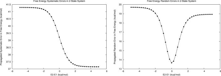
As a numerical example, let us consider a hypothetical two-state protein (hereafter referred to as M1) modeled with a force field containing 0.21 ±0.6 kcal/mol error per interaction for van der Waals contacts and 0.41 ±2.29 kcal/mol error per interaction for hydrogen bonds (this error profile is similar to what we have found for the generalized AMBER force field, i.e., GAFF). Assume that state 1 comprises 50 van der Waals and 65 hydrogen bonding interactions while state 2 comprises 60 and 70 of each, leading to overall microstate energy calculation errors of 37.2 ±18.9 kcal/mol for state 1 and 41.3 ±19.7 kcal/mol for state 2. As shown in Fig. 1, the first-order error propagation is strongly dependent on the energy gap between the two states. Propagated systematic error is dominated by the error of the lower energy microstate until the relative energies are within approximately |2| kcal/mol (assuming T=300K), where its value approaches the arithmetic mean of the two microstate systematic error values. In contrast, propagated random error begins to decrease slowly at the |2| kcal/mol region, and is minimized when the energies of the two states are equal.
Figure 1.
a) First-order propagated systematic error in free energy for M1, a model two-state system with constant energy errors (δE1 and δE2) at different relative energies. At relative energies greater than |2| kcal/mol the lower energy microstate dominates in the propagated error, but at smaller relative energies the total systematic error approaches the arithmetic mean systematic error of each microstate. b) First-order random error in free energy of the same two-state system. Random error is decreased as the energies of the two microstates approach one another.
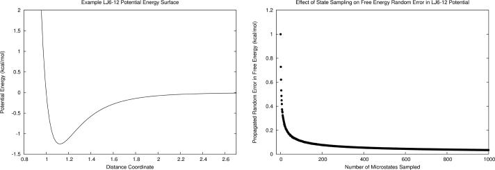
To demonstrate the effect of random error reduction due to increasing number of included microstates, we constructed a series of hypothetical ensembles (M2) in which the number of microstates is incremented by one up to one thousand. The discrete microstates were randomly selected from the potential energy surface, which was modeled as a Lennard-Jones type function (Eq. 11) with parameters ε=5.0 and σ=1.0, as plotted in Fig. 2a. The minimum of the potential well (x ≈ 1.12) was always included as a permanent global minimum microstate, and the remaining microstates were randomly selected from the potential energy surface. Each of the microstates was assigned zero systematic error and a random error of 1.0 kcal/mol. As shown in Fig. 2b, the first-order propagated random error in free energy is 1.0 kcal/mol when the ensemble contains a single microstate. When 10–20 microstates are added, the error drops below 0.2 kcal/mol. When 50–60 microstates are included, the benefit of increased local sampling begins to diminish as the propagated random error approaches zero.
Figure 2.
a) Potential energy surface of a hypothetical system (M2) modeled as a Lennard-Jones function. b) First-order propagated random error in free energy for the potential energy surface diminishes with increasing numbers of microstates included in the statistical ensemble.
| (11) |
Similar analysis can be done for the macroscopic average energy E expressed by Eq. 12:
| (12) |
where first-order error propagation yields the formula: (see supporting information for our derivation):
| (13) |
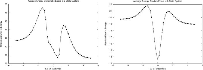
The values of propagated errors in average energy depend on (1) the probability (normalized weight) of each microstate, (2) the energy value of each microstate, (3) and the average energy itself. Returning to the M1 model system, we observed similar error propagation behaviors for average energy as for free energy in the regions where the energy gap is large or zero; however, near the |2| kcal/mol region, large “hills” of increased propagated errors now appear. The effect is more significant in the systematic error, where the propagated error value rises by about 8 kcal/mol. In addition, the width of the “funnel” representing favorable random error cancellation is narrower for average energy than for free energy.
Similarly we can investigate the propagation of systematic and random errors in entropy based on Gibb's entropy formula:
| (14) |
First-order error propagation in entropy yields the formula (see supporting information for our derivation):
| (15) |
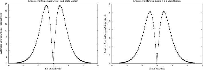
Upon applying this formula to M1, we found that at large energy gaps, the propagation of microstate systematic and random errors nears zero, and increases significantly as the energy difference decreases, but to a much smaller magnitude than the individual microstate energy errors (Fig. 4). As the energy gaps approach zero, so do the propagated errors in entropy, for both error types. Interestingly, the first-order propagation of errors in entropy was symmetric about isoenergetic points for both error types. Additionally, the “hills” of increased propagated systematic error in energy and entropy should partially cancel when combining the two terms to calculate free energy (via E-TS).
Figure 4.
a) Propagated systematic error in entropy (TS with T=300K) for M1. b) Propagated random error in entropy for M1.
Notably, the above first-order error propagation analysis is only practically reliable when microstate modeling errors are small. However, effects such as the random error reduction behavior observed here also occur at higher orders as demonstrated in the following section.
Beyond First Order
In order to establish more practical error analysis methods, which can be generally applied to even large microstate modeling error magnitudes, we have extended our error propagation analysis to higher-order schemes. Two strategies were employed. First, we continued the Taylor series expansion-based approach, where analytical forms for second (Eq. 16) and fourth (Eq. 17) order error propagation were derived by assuming independent microstate energies and considering only up to the second moments of the error probability density functions.9 Second, we conducted Monte Carlo (MC) error simulations, in which errors were randomly drawn from a Gaussian probability density function centered at a given systematic error with a standard deviation equal to the given random error. The simulated errors were then added to the given energies and free energy was computed 107 times to ensure convergence. The resulting shift in sample mean and standard deviation were used to represent propagated systematic and random error in the free energy.
| (16) |
| (17) |
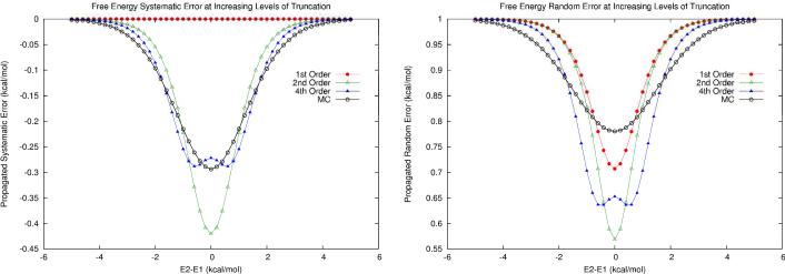
We first examined a two-state system where the two microstates have zero intrinsic systematic error but 1.0 kcal/mol of random error. The error estimation results are summarized in Table 1 and Fig. 5. We observed that, although the individual microstates contained no systematic errors, the microstate random errors lead to a propagated systematic error in the computed free energy. The first-order error analysis completely neglects this effect, yet here it yields a random free energy error estimate closest to the MC estimate. Systematic free energy errors nearly converge at fourth order, but random errors seem to converge more slowly. The MC estimates validate the previous observation that random errors are diminished as the two microstates are more equally weighted in the ensemble.
Table 1.
Propagated errors in free energy at different levels of truncation at the isoenergetic point for small microstate energy errors.
| 1st order | 2nd order | 4th order | MC results | |
|---|---|---|---|---|
| Systematic Error | 0 | −0.420 | −0.272 | −0.293 |
| Random Error | 0.707 | 0.569 | 0.653 | 0.780 |
Figure 5.
Error Propagation of two-state system with no systematic microstate energy errors and random microstate energy errors of 1.0 kcal/mol. a) Propagated systematic errors at first order (red), second order (green), fourth order (blue), and the Monte Carlo estimation (black). b) Propagated random errors at the same levels of truncation.
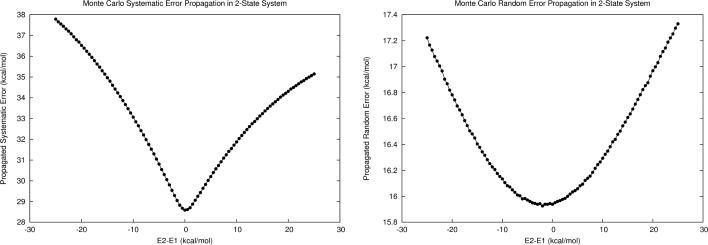
In Fig. 5, we see how increasing levels of truncation begin to converge toward MC results for small error magnitudes. However, the magnitudes of microstate energy errors for sizeable proteins and common force fields are usually much larger. To investigate the behavior of larger microstate energy errors, we re-visited model system M1. As introduced earlier, this system includes two microstates with sizeable microstate energy errors of 37.1 ±18.9 and 41.3 ±19.7 kcal/mol respectively. As shown in Figure 6, the MC error propagation results show very different behavior than predicted by first-order formulas. For instance, contrary to the prediction from the first-order analysis, the propagated systematic errors (Fig. 6a) are lower in magnitude than both of the microstate energy systematic errors, even at high energy gaps. The propagated random errors (Fig. 6b) also fall below the microstate random errors but to a lesser extent than what is predicted by first-order analysis (compare to Fig. 1b). In Table 2, the MC estimates at the isoenergetic point are compared with the corresponding low-order error propagation formulas. It is clear that low-order error analysis is not sufficient to estimate propagated errors when microstate energy errors are large. Thus for large microstate energy errors, the MC method should be employed.
Figure 6.
Monte Carlo estimation of propagated errors in the free energy of M1, a hypothetical 2-state protein system with large microstate energy errors. a) Propagated systematic error. b) Propagated random error.
Table 2.
Propagated errors in free energy at different levels of truncation at the isoenergetic point for M1.
| 1st order | 2nd order | 4th order | MC results | |
|---|---|---|---|---|
| Systematic Error | 39.23 | −117.6 | 20480 | 28.60 |
| Random Error | 13.67 | 156.2 | 20440 | 15.94 |
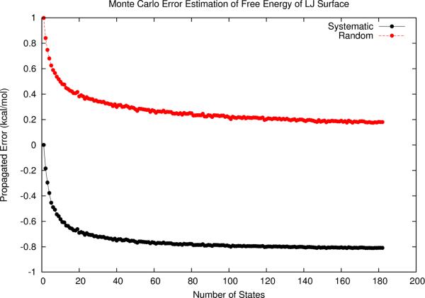
The discrepancy between low-order formulas and MC estimates led us to revisit the “random error reduction” behavior as observed in the context of first-order analysis. To examine the generality of this effect, we again examined the model system M2 described by the Lennard-Jones surface of Eq. 11. As detailed earlier, each microstate sampled in the ensembles of increasing size included no systematic error but 1.0 kcal/mol random error. From the MC results (Fig. 7), we found that random errors indeed follow similar error reduction behavior (compare with Fig. 2b). However, systematic errors are simultaneously introduced. This general “random error reduction” behavior reconfirms the notion that ensemble quantities have less random modeling errors in comparison with single global minimum microstate energies, and therefore should be preferred as energetic score functions, provided that systematic errors are estimated and removed.
Figure 7.
Monte Carlo estimation of free energy errors as a function of increased local sampling of the example Lennard-Jones surface. As more states are sampled, each with its own 1.0 kcal/mol random energy error, the propagated free energy random error is decreased, while systematic error is introduced.
A Simulated Example
To demonstrate a possible error-handling protocol based on the observations of this work, we built a model system (M3) resembling various states of a small protein undergoing folding. The model ensemble comprised 5 (macro)states, each represented by 100 microstates. Such a dataset might arise from a clustering of snapshots from molecular dynamics simulations as done in the development of Markov models of protein folding, for example as seen in Bowman et al..10 In this model system, the 5 states have their average energies randomly selected from a uniform distribution in the range (−100, 0) kcal/mol. Each component microstate was assigned a “true” energy randomly selected from a normal distribution centered at the corresponding state average energy with a standard deviation of 3.0 kcal/mol. In addition, each state was given a random average number of hydrogen bonds, selected from a uniform distribution in the range (25, 55). The number of hydrogen bonds of each microstate was then randomly selected from a normal distribution centered on the average value of the corresponding state with a standard deviation of 1. The same procedure was employed to assign van der Waals contacts, with the states randomly assigned in the range of (40, 80) and microstate deviations selected from a normal distribution with a standard deviation of 2. The energy function is assumed to contain errors of 0.21 ±0.60 for van der Waals contacts and 0.41 ±2.29 for hydrogen bonds. These parameters lead to a set of “measured” microstate energies that are shifted from their “true” values based on the propagated microstate energy errors.
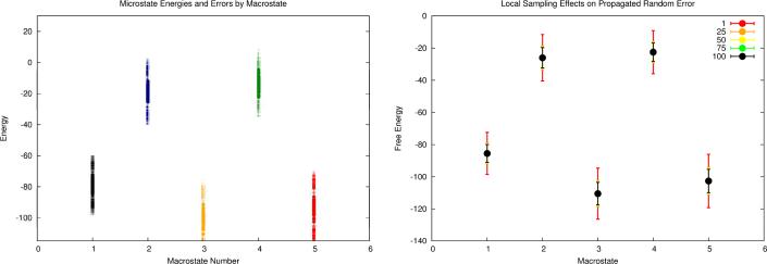
We now aim to compute free energy differences between the 5 states given the set of erroneous microstate energies. The procedure is illustrated in Fig. 8. The first step in an error-handling free energy computation would be to analyze each microstate for its intramolecular interactions. The microstate contact counts are displayed in Fig. 8a, which highlights the similarity of molecular contacts within each of the five states. In step two, by following our fragment-based error propagation procedure, we calculate the systematic and random errors of the microstate energies, which are shown in Fig. 8b. In the third step, the energies of all microstates are corrected by removing systematic errors. The resulting sets of corrected microstate energies and associated error bars are displayed in Fig. 8c. Finally, independent MC error simulations are conducted for each of the 5 states. These simulations give rise to the final estimates of the free energies of all five states along with their associated uncertainties. The black dots and the black error bars in Fig. 8d show the final estimated free energy values and the corresponding random errors when all 500 microstates are sampled. For example, the free energy of state 3 is estimated to be −110.5 ±6.97 and the free energy of state 5 is −102.6 ±7.24. The free energy difference between these two states is calculated to be 7.86 ±10.1. Here, the uncertainty of the free energy difference is evaluated as the Pythagorean sum of the error bars of the two states. In this model system, we also observe the random error reduction effect. We analyzed the ensemble results with the number of the sampled microstates per state equal to 1, 25, 50, 75, and 100. As shown in Fig. 8d, if only one microstate is sampled for each state, the error bars are very large, but when more than 25 microstates are included, the error bars are significantly reduced.
Figure 8.
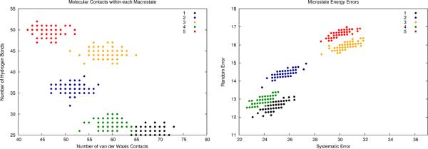
Results of an error-handling free energy computation on a simulated ensemble (M3). a) The microstates are clustered into (macro)states yielding structures containing roughly the same numbers of molecular contacts. b) An analysis of each microstate leads to systematic and random errors in each microstate energy. c) Systematic microstate energy errors are corrected, and each microstate now only has random error to be propagated. d) A Monte Carlo error propagation within each state results in a free energy estimate along with random error, which is reported with the calculated free energies. Note how the error bar magnitudes decrease with increased local sampling (1, 25, 50, 75, and 100 samples were investigated). Now free energy differences between macrostates have less error (due to the removal of systematic errors) and include estimated uncertainties due to using imperfect energy functions.
Unfortunately, MC error propagation is unable to estimate the introduction of systematic shifts in free energy due to microstate random errors. Systematic shifts in free energy estimations depend on both the magnitudes of microstate random errors and the distribution of calculated microstate energies. In this instance these shifts in free energy had a range of magnitudes from 0.25 to 4.5 kcal/mol, which suggests that these systematic errors would not cancel completely when taking free energy differences. Furthermore, low-order systematic error formulas failed to estimate these shifts (See Table 3). For this reason, it is important to be attentive to the magnitudes of the final propagated error bars, since they give a direct value of random uncertainty and a rough indication of the presence systematic shifts.
Table 3.
Free energy values (kcal/mol) from the simulated ensemble.
| State | True ΔA | Calculated ΔAa | Error in ΔA | Calculated Uncertainty in ΔAa | True Shift in A | Calculated Shift in Aa,b |
|---|---|---|---|---|---|---|
| 1 | 25.0 | 30.2 | 5.24 | ±8.89 | −0.702 | 3730 |
| 2 | 84.5 | 85.0 | 0.495 | ±9.40 | −4.52 | 6590 |
| 3 | 0 | 0 | 0 | ±9.88 | −0.258 | −2840 |
| 4 | 88.0 | 93.5 | 5.55 | ±8.98 | −1.36 | 2880 |
| 5 | 7.86 | 5.09 | −2.77 | ±10.0 | −3.47 | −9860 |
Columns marked with the superscript “a” represent quantities that could be calculated in a real computational experiment while the remaining quantities come from the simulated ensemble and are generally not known in a real computational experiment.
The calculated shifts in A come from Taylor series estimation up to 4th order. ΔA values are computed with state 3 (lowest energy state) as a reference.
Conclusions
This work serves as an extension of our previously proposed methods3–4 for estimating microstate energy errors by describing their propagation when statistical mechanical variables such as free energy are estimated. The main benefits of such an analysis are that (1) estimated systematic errors can be corrected, and (2) random errors can provide uncertainty estimates when simulation results are reported. Interestingly, we found that propagated random errors in computed free energies can be reduced by increasing the local sampling of potential energy surfaces. This suggests that, analogous to the enthalpy-entropy compensation effect, there exist correlated interplays between energy modeling errors and state sampling. As errors in an energy model are introduced, one can take advantage of state sampling to minimize the associated errors in free energy estimations. We also observed the effect of partial systematic error cancelation between energy and entropy in free energy (Figures. 1, 3, and 4) through the presence of the “hills” of propagated error in energy which are diminished when entropy and its associated error are subtracted to produce free energy and its associated error.
Figure 3.
Propagated error in the average energy for M1. a) The first-order propagated systematic error dramatically increases then decreases as the energy difference narrows. b) The propagated random error also increases slightly as the energy difference narrows, but then reaches a global minimum when the microstate energies are equal.
The error propagation formulas derived in this work approximate the accumulation of microstate energy errors by using truncated Taylor series. Higher orders of Taylor series expansions could be utilized, but this is expected to yield more complicated error propagation formulas than presented here. For very large microstate energy errors, Monte Carlo error estimation may be necessary to correctly estimate propagated random error magnitudes. A second assumption made in this work is that microstate energies are independent from one another, which may not be a valid approximation when sampling along a molecular dynamics trajectory. Thus special care will need to be taken to ensure at least quasi-independent state sampling in future applications. Further assessing the validity of these approximations and the application of error propagation techniques to the simulation of biomolecular systems will be addressed in future work.
Supplementary Material
Dedication.
I (KMM) first met Wilfred when he spent a sabbatical at UCSF in the laboratory of the late Peter Kollman in the late 1980s. He taught a very interesting class on statistical mechanics, simulation and free energy methods while at UCSF and I still have his notes to this day. Wilfred has been a wonderful teacher, mentor, friend and colleague in the intervening years, which I count as a blessing. I congratulate him on the occasion of his 65th birthday and I look forward to interacting with Wilfred for many years to come!
Acknowledgements
The authors thank Adrian Roitberg, Erik Deumens, Ben Roberts, Danial Dashti, and Melek Ucisik for helpful discussions. This work was funded by the National Institutes of Health (http://nih.gov GM044974 and GM066689 to K. M. M.) and the National Science Foundation (MCB 0919983 to W.Y.)
Footnotes
Supporting Information Our derivations of low-order derivatives of free energy and error propagation formulas are given in the supporting information. This material is available free of charge via the Internet at http://pubs.acs.org.
References
- 1.Helgaker T, Klopper W, Tew DP. Quantitative quantum chemistry. Mol. Phys. 2008;106(16–18):2107–2143. [Google Scholar]
- 2.Shaw DE, Maragakis P, Lindorff-Larsen K, Piana S, Dror RO, Eastwood MP, Bank JA, Jumper JM, Salmon JK, Shan YB, Wriggers W. Atomic-Level Characterization of the Structural Dynamics of Proteins. Science. 2010;330(6002):341–346. doi: 10.1126/science.1187409. [DOI] [PubMed] [Google Scholar]
- 3.Faver JC, Benson ML, He X, Roberts BP, Wang B, Marshall MS, Sherrill DC, Merz KM. The Energy Computation Paradox and ab initio Protein Folding. PloS ONE. 2011;6(4):e18868. doi: 10.1371/journal.pone.0018868. [DOI] [PMC free article] [PubMed] [Google Scholar]
- 4.Faver JC, Benson ML, He X, Roberts BP, Wang B, Marshall MS, Kennedy MR, Sherrill DC, Merz KM. Formal Estimation of Errors in Computed Absolute Interaction Energies of Protein-ligand Complexes. J. Chem. Theory Comput. 2011;7(3):790–797. doi: 10.1021/ct100563b. [DOI] [PMC free article] [PubMed] [Google Scholar]
- 5.Merz KM. Limits of Free Energy Computation for Protein-Ligand Interactions. J. Chem. Theory Comput. 2010;6(5):1769–1776. doi: 10.1021/ct100102q. [DOI] [PMC free article] [PubMed] [Google Scholar]
- 6.Taylor JR. An introduction to error analysis: the study of uncertainties in physical measurements. 2nd ed. University Science Books; Sausalito, Calif: 1997. p. xvii.p. 327. [Google Scholar]
- 7.(a) Susnow R, Nachbar RB, Schutt C, Rabitz H. Sensitivity of Molecular-Structure to Intramolecular Potentials. J. Phys. Chem. 1991;95(22):8585–8597. [Google Scholar]; (b) Wong CF. Systematic Sensitivity Analyses in Free-Energy Perturbation Calculations. J. Am. Chem. Soc. 1991;113(8):3208–3209. [Google Scholar]; (c) Gilson MK. Sensitivity analysis and charge-optimization for flexible ligands: Applicability to lead optimization. J. Chem. Theory Comput. 2006;2(2):259–270. doi: 10.1021/ct050226y. [DOI] [PubMed] [Google Scholar]
- 8.Ucisik MN, Dashti DS, Faver JC, Merz KM. Pairwise Additivity of Energy Components for Protein-Ligand Binding: HIV II Protease-Indinavir Case. J. Chem. Phys. 2011;135:085101. doi: 10.1063/1.3624750. [DOI] [PMC free article] [PubMed] [Google Scholar]
- 9.Winzer PJ. Accuracy of error propagation exemplified with ratios of random variables. Rev. Sci. Instrum. 2000;71(3):1447–1454. [Google Scholar]
- 10.Bowman GR, Beauchamp KA, Boxer G, Pande VS. Progress and challenges in the automated construction of Markov state models for full protein systems. J. Chem. Phys. 2009;131(12) doi: 10.1063/1.3216567. [DOI] [PMC free article] [PubMed] [Google Scholar]
Associated Data
This section collects any data citations, data availability statements, or supplementary materials included in this article.


