Extracting Conformational Memory from Single-Molecule Kinetic Data

Abstract

Single-molecule data often comes in the form of stochastic time trajectories. A key question is how to extract an underlying kinetic model from the data. A traditional approach is to assume some discrete state model, i.e. a model topology, and to assume that transitions between states are Markovian. The transition rates are then selected according to which best fit the data. However in experiments, each apparent state can be a broad ensemble of states or can be hiding multiple inter-converting states. Here we describe a more general approach called the non-Markov Memory Kernel (NMMK) method. The idea is to begin with a very broad class of non-Markov models and to let the data directly select for the best possible model. To do so, we adapt an image reconstruction approach that is grounded in Maximum Entropy. The NMMK method is not limited to discrete state models for the data; it yields a unique model given the data; it gives error bars for the model; it does not assume Markov dynamics. Furthermore, NMMK is less wasteful of data by letting the entire data set determine the model. When the data warrants, the NMMK gives a memory kernel that is Markovian. We highlight, by numerical example, how conformational memory extracted using this method can be translated into useful mechanistic insight.

1 Introduction

It is now routine to measure single-molecule (SM) trajectories of ion-channel opening/closing events or folding/unfolding transitions of proteins and nucleic acids [1, 2, 3, 4, 5]. Single molecule trajectories show transitions of a molecule from one conformational state to another. For instance in SM force spectroscopy, the trajectory includes transitions between a high force state (folded state) and low force state (unfolded state). Individual states can exhibit what is called “conformational memory” [1]. Broadly speaking, when a state has conformational memory, the dwell time in that state is not distributed as a single exponential. Alternatively, one can say that in bulk, the relaxation is not single exponential. For example, the folding of phosphoglycerate kinase monitored by bulk fluorescence experiments following a temperature jump [6] hints at a kinetically heterogeneous process; SM fluorescence experiments find that adenylate kinase apparently shows no less than six folding intermediates [8].

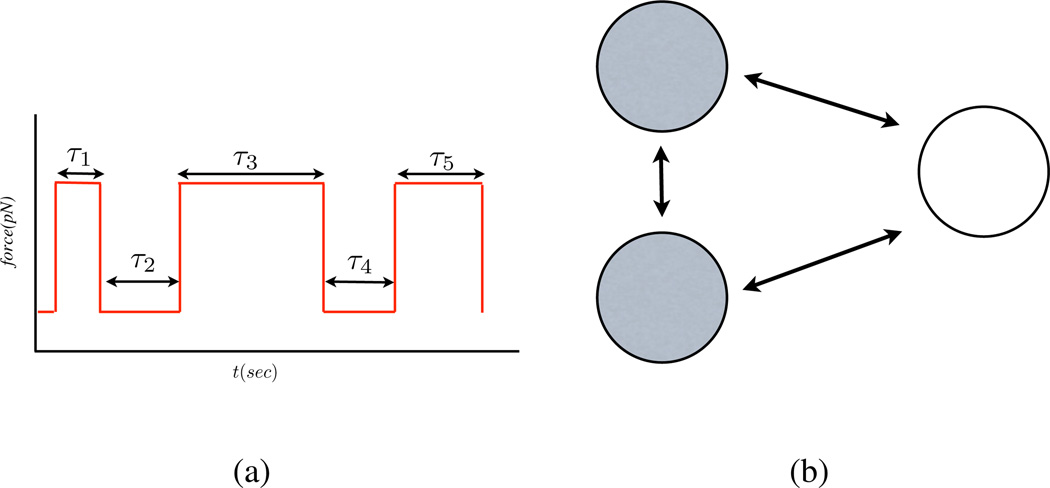
Fig.(1) is a cartoon illustration of how conformational memory can arise. In this cartoon example, the origin of the conformational memory is simple to understand. The low force state in Fig.(1(b)) is made up of two microscopic states; it is called an aggregate. The dwell time distribution in the low force state is therefore not a single-exponential because the low force state is composed of two inter-converting states indistinguishable in this particular experiment. Such models are called Aggregated-Markov (AM) models [9, 10, 11]. The states within an observable aggregate are assumed to exchange with each other via Markov processes. There are well-known limitations in using AM models in data analysis. First, they require advance knowledge of the topology of the underlying kinetic states. By topology, we are referring to the kinetic relationships among the states, usually expressed as sets of arrows connecting the underlying states, see Fig. (1(b)). As a consequence, the AM approach does not make full use of the data set -it forces the data onto a model rather than to let the data tend towards a model. Second, if there are fewer independent observables than rates in the model, then AM models are not unique; many different models would fit the data [12]. For example, a 3-state system with two observable aggregates requires 6 rate coefficients. However, only 4 independent parameters are determinable from such data. This problem is often solved by using some symmetry relationship –for example by assuming that some rates are identical [13], or by performing additional experiments that give orthogonal information [14]. Third, AM models require the assumption that transitions are Markovian and that there are a finite number of states. In reality, there could, instead, be a continuous manifold of underlying states [15], fluctuating rates [20], or strong memory effects that can give rise to heavy-tail statistics [21]. Points one and three are also limitations of a related strategy tailored for noisy data, called Hidden Markov (HM) modeling [25, 7]. HM models are commonly used when the microscopic state in which the molecule is found are obscured by the noise. Thus HM modeling techniques can be useful in extracting aggregated Markov models from data. That is, the HM and AM models are not mutually exclusive. The stochastic rate models is another possible description of a system with memory where the escape from a complex state is decribed using a rate which is a stochastic variable, in general depending on time [22]. Yet another method is the Multiscale State Space Network, which is useful for mapping out the interconnectivity of conformational state space of a protein from a continuously varying observable [23]. Alternatively, the conformational state space of single proteins has been described using a Langevin equation with a memory kernel fit to data [24].

Figure 1.

The experiment can only distinguish between two observable states - a high force and a low force state - for this example drawn from SM force spectroscopy. (a) A cartoon of a stochastic time trajectory shows the discrete transitions of SM between two conformational states (one extended and the other not). τ denotes the amount of time the molecule dwells in each successive state. (b) The AM model. Here the dark shaded state (the high force state) represents the folded state while the un-shaded state (low force state) represents the unfolded state. For this example, the dark shaded state is composed of two underlying microscopic states which transition between themselves and to all other states via a Markov process. The dwell time distribution in this state is correspondingly biexponential.

Here we describe an alternative approach to kinetic modeling. The idea is to start with a very broad class of kinetic models. We subsequently use the data from SM time traces and the tools of Maximum Entropy (MaxEnt) [15, 16, 26, 27, 28] to select the best model from this class. The purpose of this approach is to avoid biasing our analysis or wasting data by forcing the data ahead of time to fit a predetermined model. Rather we let the data determine the model.

We call our approach the Non-Markov Memory-Kernel (NMMK) method. Here the underlying system kinetics are modelled using continuous memory kernels rather than using explicit states such as in AM and HM modeling. In the NMMK method, the memory kernel itself is the model. It predicts the full dynamics without the need for any associated assumptions about kinetic rates or topologies. Thus a Markov model (a model with no memory) emerges from the NMMK method only if it is warranted by the data. In many ways this method complements AM and HM modeling methods described above as well as approaches for inferring rate distributions –also called rate spectra– from raw data; these include a hybrid method of of Maximum Entropy and nonlinear least squares (MemExp) [16] as well as a variety of other methods [17]. Such methods seem less successful when applied to rate distributions which cannot be described by the sum of many exponentials [17]. Other efforts in describing sequential multistep reactions [18] are specific to exponential rates or stochastic rates sampled from a Gaussian distribution [19].

Here we focus on some clear distinguishing features of the NMMK method: the model extracted is unique, transitions between states are not assumed Markovian from the onset, a topology is not assumed a priori, our variational method yields the time it takes for the memory in each state to decay to zero and the method gives error bars on the model it predicts. We also discuss what features we should expect in the memory kernel for the special case when the observed state is composed of an aggregate of states.

2 Theoretical Methods

2.1 The Non-Markov Memory Kernel Model approach

Here we illustrate how the NMMK method works on simulated data. In the analysis of noisy time traces of SM data, investigators first pick out transitions and obtain both marginal dwell time histograms for each state as well as conditional dwell time histograms for each pair of state (processes entirely described by marginal dwell histograms for each state are called renewal processes [30]). Furthermore, for AM models, no additional information is contained in higher order conditional histograms [9].

For instance, from Fig.(1(a)) the dwell time distribution in the low force state is obtained by histogramming τ₂, τ₄, … In a follow-up publication where we will tackle real experimental data, we use change-point algorithms [31] for detecting transitions in noisy data in a model independent way. That is, unlike the HM or AM approach, transitions are picked out from data in a way which does not depend on the topology assumed a priori.

The NMMK model describes the kinetics in terms of a generalized master equation with a memory kernel κ(t), as follows

$$ḟ(t)=-{\displaystyle {\int }_0^t}d\mathrm{\tau }\mathrm{\kappa }(\mathrm{\tau })f(t-\mathrm{\tau })\equiv -\mathrm{\kappa }(t)*f(t)$$ (1)

where f (t) denotes a dwell time distribution in a particular state obtained from data ¹. When we talk about a model we will be referring to the memory kernel. It gives us a dynamical picture of a state by telling us how the memory in a state decays.

Note that if the dwell distribution, f (t), in a particular state is single exponential, then the resulting κ(t) is a delta function. This is the signature of a memoryless, i.e. Markov, process. Put another way, if the memory kernel for some state is a delta function, we conclude that this state is a single state whose transitions to its neighbors satisfy the Markov property.

2.2 The AM model shows clear signatures in the memory kernel

Suppose some state A is an aggregate of indistinguishable discrete states. We show in the appendix that AM models always give rise to multi-exponential dwell time distributions. What memory kernel should we expect for state A?

In this case, the most general dwell time distribution in this state is

$$f(t)={\displaystyle \sum _i}{c}_i{e}^{-{\mathrm{\lambda }}_{i}t}.$$ (2)

An exponential decay with N components can arise in cases where the state is an aggregate of N states. In Laplace space Eq. (1) is

$$s\mathrm{f̂}(s)-f(0)=-\mathrm{\kappa ̂}(s)\mathrm{f̂}(s).$$ (3)

Substituting Eq. (2) into Eq. (3) yields

$$-\mathrm{\kappa }(t)={ℒ}^{-1}(s-\frac{{\displaystyle {\sum }_i}{c}_i}{{\displaystyle {\sum }_i}\frac{c_i}{{\mathrm{\lambda }}_i+s}})\equiv {ℒ}^{-1}O$$ (4)

where ℒ⁻¹O denotes the inverse Laplace transform of O. We will perform the inverse Laplace transformation by expressing O using partial fractions as ∑_m h_m/(s + σ_m) + K (for constant K). This gives

$$-\mathrm{\kappa }(t)={\displaystyle \sum _m}{e}^{-{\mathrm{\sigma }}_{m}t}{h}_m+K\mathrm{\delta ̃}(t)$$ (5)

where δ̃(t) is defined by the property ${\displaystyle {\int }_0^{\mathrm{\infty }}}y(t)\mathrm{\delta ̃}(t)\mathit{\text{dt}}=y(0)$. The explicit form of Eq. (5) is:

$$-\mathrm{\kappa }(t)={\displaystyle \sum _{m=1}^{n-1}}{e}^{-{\mathrm{\sigma }}_{m}t}\left(\frac{-{\displaystyle {\prod }_{i=1}^n}({\mathrm{\lambda }}_i-{\mathrm{\sigma }}_m)}{{\displaystyle {\prod }_{j=1,j\ne m}^{n-1}}({\mathrm{\sigma }}_j-{\mathrm{\sigma }}_m)}\right)-\frac{{\displaystyle {\sum }_i}{c}_i{\mathrm{\lambda }}_i}{{\displaystyle {\sum }_i}{c}_i}\mathrm{\delta ̃}(t)$$ (6)

where the {σ_i} are the zeroes of ${\displaystyle {\sum }_i}{c}_i\frac{1}{{\lambda }_i+s}$.

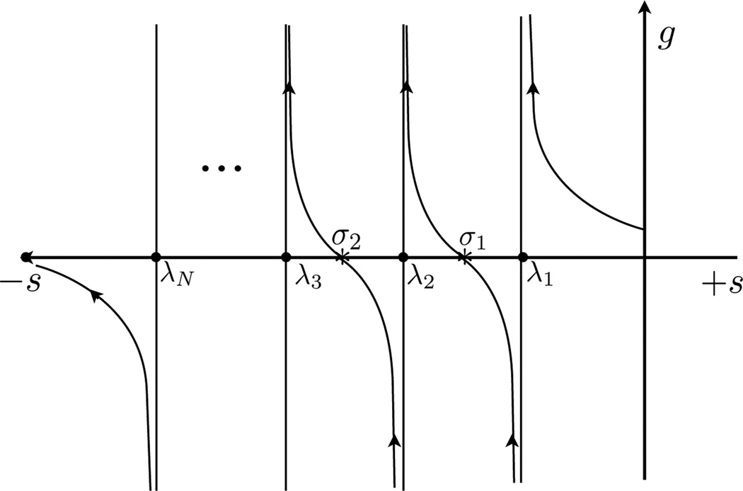
For the special case that all {c_i}’s in Eq. (2) are positive, all parameters {σ_m, h_m} are also positive. To see this explicitly, consider a plot of f̂(s), see Fig. (3), where it is clear that λ₁ < σ₁ < λ₂ < σ₂… < σ_n−1 < λ_n. The signs of the {h_m} are then determined from its explicit form in Eq. (6). From this ordering and Eq. (6), it follows that all {σ_m, h_m}’s are positive.

Figure 3.

Pole and zero structure of g ≡ f̂ (s). Dots denote poles, asterisks denote zeroes.

The structure of the zeroes and poles is more complicated when some of the {c_i}’s are negative, which can apply in instances where detailed balance is violated in the underlying AM model. Nonetheless, we can still rank order the zeroes and poles to determine the sign of {σ_m, h_m}.

The type of structure we expect in the memory kernel from an AM model is given by Eq. (6). Eq. (6) captures a sharp spike in the memory kernel at t = 0 (the hallmark of a Markov process) in addition to components present at later times which describe the relaxation of the memory kernel.

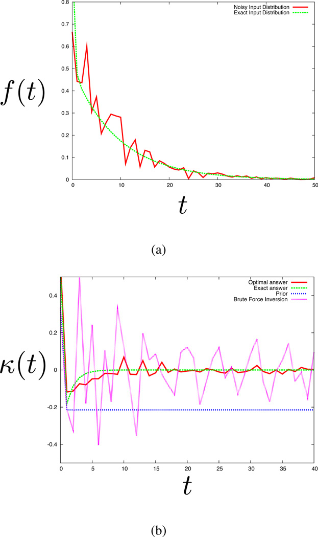
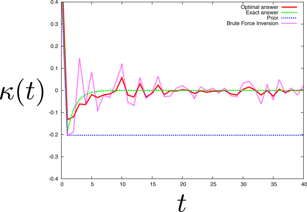
While in its full generality Eq. (6) looks daunting, consider a simple biexponential dwell time distribution with positive {c₁, c₂}. This dwell describes the decay from an aggregated state with two different timescales, a faster and a slower timescale. In this case, the memory kernel is a sharp positive spike at the origin (the delta function) followed by a dip below zero and then followed by an exponential rise back to zero. See the green curve in Fig. (4(b)) for an example of this behavior. At the origin, the memory kernel’s sharp positive spike says that the decay is memoryless. At the next time step, the slower timescale becomes relevant and reduces the effective rate of escape from this state. This coincides with the negative component of the memory kernel. In other words, the slower timescale introduces memory in the memory kernel; it introduces mathematical structure beyond the single spike at the origin.

Figure 4.

Extraction of the memory kernel from data. (a) Time trace data, where the green curve is double exponential function and the red curve is the fictitious data obtained by adding 40% noise. (b) The memory kernel. The green curve is the exact answer, the pink curve is the one obtained by brute force (i.e. direct) inversion, the blue curve is the prior, and the red curve is the solution obtained by image reconstruction (the optimal answer). See the text for details.

Memory kernels arising from multi-exponential dwell time distributions are helpful in building intuition because the form for the coinciding memory kernels have analytic mathematical forms. We have just shown how additional states yield effective memory in the system. Given an AM model, the structure of the memory kernel can then be interpreted according to the presence of aggregates of discrete states. However AM models are idealizations of real data and the structure in the memory kernel can be interpreted differently. For example, the structure in the memory kernel can be interpreted in the context of a diffusion model in a rough energy landscape - a model recently used to describe the dwell in the unfolded state of phosphoglycerate kinase we discussed earlier [6]. Alternatively, we are free to interpret the memory kernel as a model where the rates themselves are stochastic variables. We argue here that the memory kernel in itself provides a model -it dictates the way in which the memory decays to zero within error as well as the amount of time this takes.

We now turn our attention to developing a robust algorithm for extracting memory kernels from noisy histograms. Answering this question will help us answer questions like “is a Markov model (the most basic of all models normally taken for granted) warranted by the data?”.

2.3 An algorithm for extracting the memory kernel

As noted earlier, transitions between states in SM trajectories are rarely as clear as shown in Fig. (1(a)). Rather, transitions are obscured by noise. In this case, a dwell distribution like f (t) would be obtained by using a model-independent change-point algorithm to detect transitions in the real noisy data [31]. That is, unlike HM models, the change-point algorithm would pick out significant transitions in the data without committing to a particular model from the onset. The output of this procedure is a “denoised time trace” like the one given in Fig. (1(a)). The amount of time spent in each state is histogrammed. Since data is finite, the histograms themselves are noisy.

The numerical extraction of the memory kernel from noisy histograms can be mapped onto an adaptation of the method of image reconstruction [15, 26, 27, 28]. Briefly, the goal of image reconstruction is to obtain an image, I, from data, D, where data and image are related by a linear transform G. That is D = G * I. Direct inversion of the data, (G_*⁻¹)D, would be numerically unstable for noisy data so we use the variational procedure of image reconstruction to regularize the operation and obtain a reconstructed image. The variational procedure is based on the principle of Maximum Entropy.

The analog of Eq. (1) in discrete time is

$$f_{j+1}-f_j=-{\displaystyle \sum _{k=0}^j}{f}_k{\mathrm{\kappa }}_{j-k}.$$ (7)

Here the memory kernel plays the role of the image. The important difference between Eq. (7) and standard image reconstruction is the operator G. Our operator in Eq. (7) contains noisy data. Our goal is to derive a variational procedure for extracting the memory kernel with such an operator. We do so by defining an objective function which we will optimize with respect to each κ_j in order to obtain our reconstructed memory kernel.

We begin by assuming the experimental input to be in the form of a dwell time histogram with error bars for each bin. That is $f_j^{\mathit{\text{exp}}}=f_j+{\epsilon }_j$ where f_j is the theoretical value of the dwell time distribution at time point j. Brute-force inversion of $f_{j+1}^{\mathit{\text{exp}}}-f_j^{\mathit{\text{exp}}}=-{\displaystyle {\sum }_{k=0}^j}{f}_k^{\mathit{\text{exp}}}{\mathrm{\kappa }}_{j-k}$ to obtain {κ_j} is numerically unstable because noise propagates quickly as we solve κ₁ in terms of κ₀, κ₂ in terms of κ₁ and so on. Image reconstruction is used as a regularizing procedure to overcome this problem. For this reason, using $f_j^{\mathit{\text{exp}}}=f_j+{\epsilon }_j$ we write Eq. (7) as follows

$$\mathrm{\Delta }{f}_{j+1,j}^{\mathit{\text{exp}}}+{\displaystyle \sum _{k=0}^j}{f}_k^{\mathit{\text{exp}}}{\mathrm{\kappa }}_{j-k}={\mathrm{\epsilon }}_{j+1}-{\mathrm{\epsilon }}_j+{\displaystyle \sum _{k=0}^j}{\mathrm{\epsilon }}_k{\mathrm{\kappa }}_{j-k,}$$ (8)

where $\mathrm{\Delta }{f}_{j+1,j}^{\mathit{\text{exp}}}\equiv f_{j+1}^{\mathit{\text{exp}}}-f_j^{\mathit{\text{exp}}}$. The deviation of experiment and theory, the residuals, are on the right hand side of Eq. (8). We assume $\langle {\mathrm{\epsilon }}_i{\mathrm{\epsilon }}_j\rangle ={\mathrm{\sigma }}_j^2{\mathrm{\delta }}_{\mathit{\text{ij}}}$ and 〈ε_i〉 = 0. Squaring both sides of Eq. (8) and taking the average with respect to the noise, we find

$$\langle {(\mathrm{\Delta }{f}_{j+1,j}^{\mathit{\text{exp}}}+{\displaystyle \sum _{k=0}^j}{f}_k^{\mathit{\text{exp}}}{\mathrm{\kappa }}_{j-k})}^2\rangle ={\mathrm{\sigma }}_{j+1}^2+{\mathrm{\sigma }}_j^2-2{\mathrm{\sigma }}_j^2{\mathrm{\kappa }}_0+{\displaystyle \sum _{k=0}^j}{\mathrm{\sigma }}_k^2{\mathrm{\kappa }}_{j-k}^2$$ (9)

We define a χ² statistic as a sum over all time intervals

$${\mathrm{\chi }}^2\equiv {\displaystyle \sum _{j=0}^N}\frac{{(\mathrm{\Delta }{f}_{j+1,j}^{\mathit{\text{exp}}}+{\displaystyle {\sum }_{k=0}^j}{f}_k^{\mathit{\text{exp}}}{\mathrm{\kappa }}_{j-k})}^2}{({\mathrm{\sigma }}_{j+1}^2+{\mathrm{\sigma }}_j^2-2{\mathrm{\sigma }}_j^2{\mathrm{\kappa }}_0+{\displaystyle {\sum }_{k=0}^j}{\mathrm{\sigma }}_k^2{\mathrm{\kappa }}_{j-k}^2)}$$ (10)

where N here is the number of data points. For a finite sample, we may invoke the frequentist logic often used in image reconstruction [15, 26, 27, 28], and suppose that χ² = N. That is, on average, the difference between each data point and its theoretical expected value differ by their standard deviation. We then follow the logic of Maximum Entropy, which is often invoked in image reconstruction, and ask that the memory kernel be as featureless as possible given χ² = N as a constraint on the data. In other words, we now maximize the objective function, F(θ, {κ}), with respect to the set {κ_j}

$$F(\mathrm{\theta },\{\mathrm{\kappa }\})=-\mathrm{\alpha }{\displaystyle \sum _j}({\mathrm{\kappa }}_j+\mathrm{\kappa ̄})\text{ log }\left(\frac{{\mathrm{\kappa }}_j+\mathrm{\kappa ̄}}{{\mathrm{\Lambda }}_j+\mathrm{\kappa ̄}}\right)-\frac{\mathrm{\beta }}{2}({\mathrm{\chi }}^2-N).$$ (11)

The entropy of the memory kernel is −∑_j(κ_j + κ̄) log((κ_j + κ̄)/(Λ_j + κ̄)); {α, β} = {cos² θ, sin² θ} are the Lagrange multipliers that enforce the constraints on the data ²; Λ_j is the prior on κ_j; and κ̄ is a constant positive parameter to ensure that κ_j + κ̄ never becomes negative so that the entropy is well-defined. Our estimate of the set {κ_j} in the absence of data is therefore ${\mathrm{\kappa }}_j^0=({\mathrm{\Lambda }}_j+\mathrm{\kappa ̄})e^{-1}-\mathrm{\kappa ̄}$. By setting χ² = N, the problem is under-determined. We therefore need to use Maximum Entropy to select one of the many possible solutions for which χ² = N. In other words, the Lagrange multipliers “tune” the balance between fitting the data points on the one hand vs. “smoothing” to achieve the model closest to the prior.

Now we need to specify our prior. In the absence of any data, we should assume a simple Markov memory kernel. In our case, we set the first two points from our brute-force memory kernel (j = 0 and j = 1) –which are more reliably determined than later points– as the first two points of the prior, Λ_j. We take the rest of the prior to be flat. The idea is to take advantage of the structure of the memory kernel we know to be reliable to set our prior.

Next, the 95% confidence interval of the memory kernel is estimated assuming that the true memory kernel lies somewhere between the solution obtained by optimizing the objective function under the constraint χ² = μ ± 2σ rather than χ² = N when N is large (where the χ² distribution has μ = N and $\mathrm{\sigma }=\sqrt{2N}$). We should expect the memory kernel’s lower bound (when χ² = μ − 2σ) to be close to the brute force inversion (where χ² is strictly zero) and its upper bound (when χ² = μ + 2σ) to be closer to the chosen prior (where χ² is very large).

As an aside, we choose the Shannon-Jaynes entropy in Eq. (11) because it worked for all examples we have considered so far and it tries to minimize features in the memory kernel; we show only a small fraction of the many numerical examples we tackled in the next section. It is quite possible that other entropies, or other regularizing procedures, would also serve as acceptable substitutes to the Shannon-Jaynes entropy.

3 Results and Discussion: Proof of principle of the NMMK method

Fig. (4) shows an illustration of how NMMK methods work on a theoretical example. We first create a decay signal and then add noise to it. We imagine such a dwell distribution originates from having used a change-point algorithm to detect significant transitions in a real time trace as discussed earlier. Then, we ask how well NMMK can extract the correct underlying model. In this case, we added 30% noise to a biexponential dwell time distribution, p_j = 0.5 × 0.9^j + 0.5 × 0.05^j; the raw “data” made up in this way is shown in Fig. (4(a)).

First, as a point of reference, Fig. (4(b)) shows the memory kernel that is obtained by brute force inversion of the raw data (pink line). It is too noisy to give a good approximation to the the exact answer (green line), or even to register that there are two exponentials in the dwell distribution. The exact memory kernel (computed from Eq. (6)) is not simply a delta function, it shows more structure consistent with the presence of a second state. Now, in order to apply the NMMK method, we use only the first two points of the pink line to construct the prior (blue line). Using that prior, we then use the NMMK image-reconstruction method. The NMMK predictions are shown as the red curve. The NMMK method clearly shows a peak followed by a dip, consistent with the correct two exponentials even when the noise level is high. This example shows that while the double-exponential behavior is invisible in the time trace due to a high noise level (Fig. (4(a)), red line), the double-exponential is nevertheless detectable as the rising tail in the memory kernel obtained by the image reconstruction algorithm (Fig. (4(b)), red curve). Hence, the NMMK method appears to be a sensitive model-building strategy that can detect structure in the memory kernel (or hidden intermediate states in the language of AM), without assuming that the process is Markovian.

A good data-processing algorithm should display both sensitivity and specificity. Sensitivity means that small changes in the data originating from the underlying physics should be reflected in the corresponding model. Specificity means that irrelevant differences in the data due to noise should not be captured in the model. Figs. (4)–(9) show our tests of sensitivity and specificity of the NMMK approach.

Figure 9.

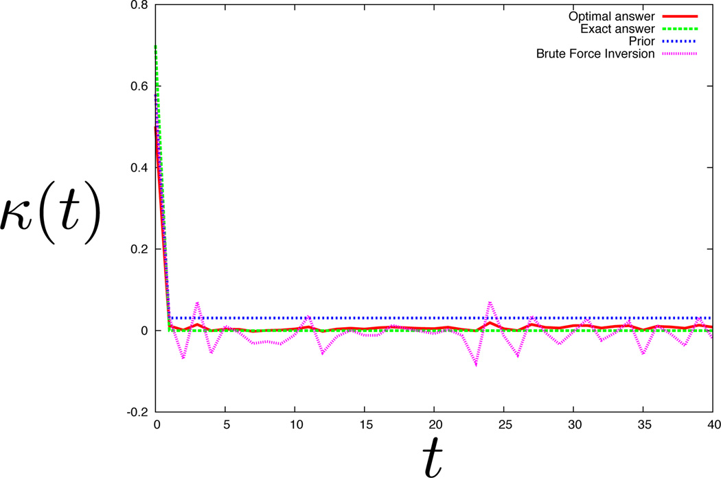
Extraction of the memory kernel from data. Same as Fig. (5), the monoexponential case, but now the noise is level is raised to 60%. These histograms have less features than their biexponential counterparts so it is easier to extract the memory kernel from such histograms at higher noise levels. The most prominent feature of the memory kernel is, somewhat surprisingly, still the sharp peak at the origin which is correct. However, at such high noise levels, the magnitude of the peak recorded at the origin is far from the theoretical exact answer.

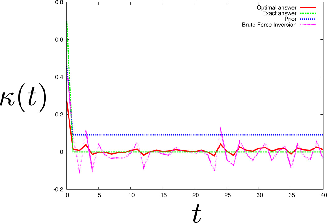
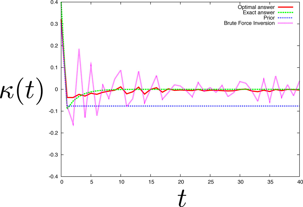
In Fig. (6), we show a memory kernel extracted from a biexponential dwell time histogram with 20% Gaussian noise. The noise is always proportional to the value of the histogram bin for each bin. Compare this to the memory kernel extracted from a dwell histogram with 40% noise from Fig. (4(b)). The biexponential nature of the dwell time distribution is apparent in both despite a large difference in the noise. Hence, NMMK shows specificity. Similarly we show specificity for memory kernels extracted from a noisy monoexponential dwell time histogram in Fig. (5) (with 40% noise) versus Fig. (9) (with 60% noise). We can extract a memory kernel for a simpler model (like the monoexponential) at higher noise levels than we can for more complex models (like biexponentials). This is because the histograms of more complex models have more features which make the NMMK method less specific.

Figure 6.

Extraction of the memory kernel from data. Same as Fig. (4) but now with 20% noise. As expected here, the optimal solution matches the theoretical solution much more closely.

Figure 5.

Extraction of the memory kernel from data. The memory kernel as a function of time when the dwell time distribution coincides with a single exponential in the presence of 40% noise. Even at 40% noise, image reconstruction can reliably extract the memory kernel and pick out the delta function expected from the noise. Other features of the memory kernel apparent from the brute force curve are interpreted as noise and the sharp peak at the origin is the only qualitatively significant feature apparent from the optimal solution.

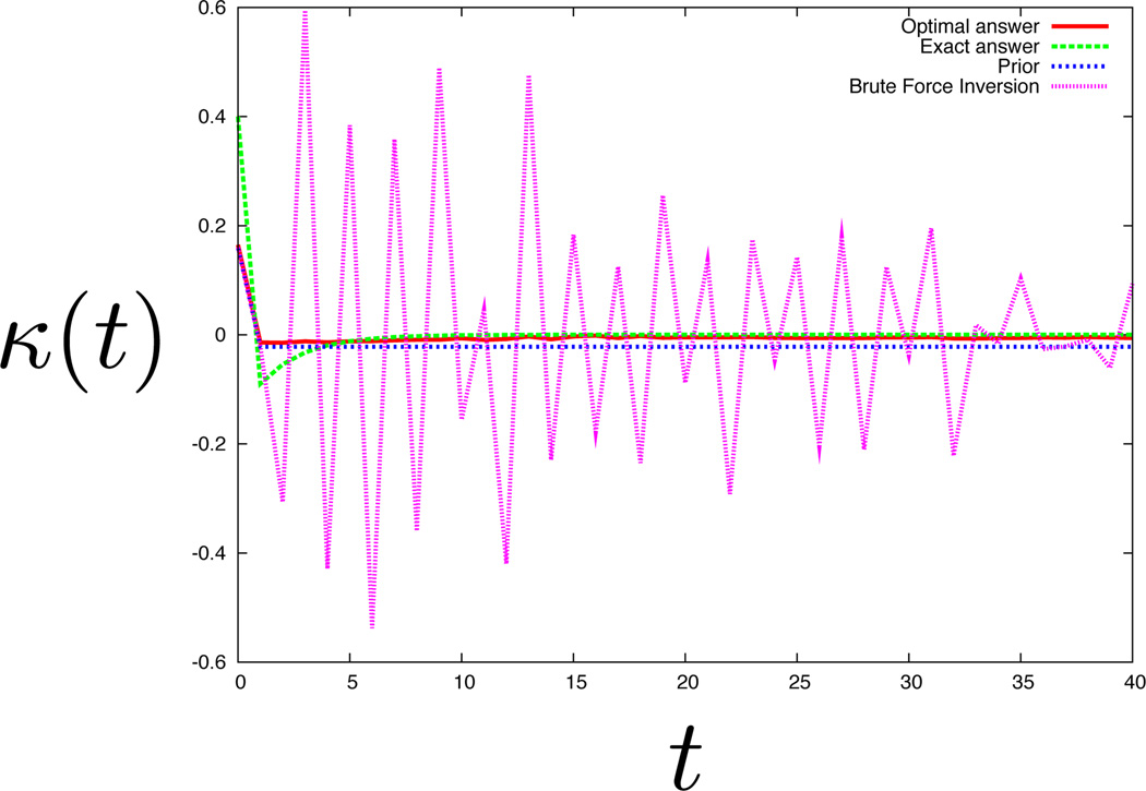
Comparing Figs. (4(b)) and (5) we find that even at 40% noise the NMMK method can distinguish monoexponential versus biexponential models. Thus NMMK is therefore also sensitive. In Fig. (8) we show that if the two decay rates of the biexponential histogram are more similar than they are for Fig. (4(b)), then the NMMK has difficulty picking out a reasonable memory kernel at 40% noise though not at 20% noise (see Fig.(7)) for the biexpoential model considered. See footnote for a brief note on noise and bin sizes ³.

Figure 8.

Extraction of the memory kernel from data. Same as Fig. (7) but now the noise is raised to 40%. For sufficiently similar rate constants, the negative dip is now impossible pick out at 40% noise. This figure should be compared to Fig. (4(b)) where the negative dip is more pronounced when the decay constants are more dissimilar. In that case, the negative dip is clearly noticeable even at 40% noise.

Figure 7.

Extraction of the memory kernel from data. Same as Fig. (6) but with a double exponential decay described by the equation 0.5 × 0.9^j + 0.5 × 0.3^j. As the two decay constants here are more similar than in Fig. (6), the negative dip expected theoretically is less pronounced and is consequently more difficult to pick out at 20%.

We have illustrated how NMMK method is used to extract memory kernels here from simple mono and biexponential histograms. We have used sums of exponentials because they are common and important in dynamical processes and simple to illustrate. However, the NMMK is not limited in any way to exponentials. NMMK can also treat processes involving a continuum of states.

4 Conclusion

Stochastic trajectories are the common form of data from SM and few-particle experiments. Such processes are often treated using AM models, where it is assumed that states are clustered together into aggregated states that can interconvert using Markov processes. To go beyond the limitations of such models, we propose an alternative, the non-Markov memory-kernel (NMMK) model. We show that the NMMK model has the following advantages: for given data, it gives a unique model (with error bars); it does not require inputting knowledge of the number of underlying states; it is readily combined with current first-principles-based image-reconstruction methods to provide a stable numerical recipe; and it can be used even when the underlying physical states are not discrete and transitions between these are not Markovian. When the data warrants a simple Markov model, the memory kernel reduces to a delta function. The NMMK is a way to harness the entire experimental output from kinetics experiments to reconstruct kinetic models with error bars. In addition, it complements the method of image reconstruction for the determination of rate distributions though NMMK is not intrinsically tied to exponential decay forms. We have only explicitly considered extracting memory kernels from dwell histograms where the time-ordering information of dwells is lost. However, our method readily generalizes to the analysis of conditional and higher-order histograms if such data is available. It is worth investigating whether our NMMK formulation could be adapted to treat time-ordered data explicitly rather than processed data like histograms.

Figure 2.

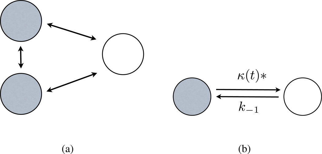
AM models and NMMK models. (a) AM model with an aggregated shaded state. (b) The AM model formulated as a NMMK model. The AM model is a special case of the NMMK model. See text for details.

Appendix

Deriving dwell time distributions for Aggregated Markov (AM) models

We first summarize the necessary theory and notation from AM models [9, 10, 12, 29]. We consider Markov states that are aggregated into s distinguishable groups, which we simply call aggregates. We define the Markovian rate matrix Q whose rows sum to zero. The submatrix Q_αβ is the rate matrix connecting the states in aggregate α to those in β. The individual matrix elements $Q_{\mathrm{\alpha }\mathrm{\beta }}^{\mathit{\text{kl}}}$ within Q_αβ for α ≠ β are the physical values for the rates connecting the k^th state in aggregate α to the l^th state in aggregate β.

Aggregate α has n_α underlying states, where ∑_α n_α = N. The general joint probability density for the dwell time t₁ in the α₁ aggregate followed by a dwell of t₂ in α₂ and so forth, denoted as f_α1…αr (t₁ …t_r), is [9]:

$$f_{{\mathrm{\alpha }}_1\cdots {\mathrm{\alpha }}_r}(t_1\cdots t_r)={\mathrm{\pi }}_{{\mathrm{\alpha }}_1}\text{exp }({\mathbf{Q}}_{{\mathrm{\alpha }}_1{\mathrm{\alpha }}_1}{t}_1){\mathbf{Q}}_{{\mathrm{\alpha }}_1{\mathrm{\alpha }}_2}\times \text{ exp }({\mathbf{Q}}_{{\mathrm{\alpha }}_2{\mathrm{\alpha }}_2}{t}_2)\cdots \text{exp }({\mathbf{Q}}_{{\mathrm{\alpha }}_r{\mathrm{\alpha }}_r}{t}_r){\displaystyle \sum _{\mathrm{\beta }}}{\mathbf{Q}}_{{\mathrm{\alpha }}_r\mathrm{\beta }}{\mathbf{u}}_{\mathrm{\beta }}$$ (12)

where u_β is a column vector of length n_β whose elements are all equal to 1, and Π_α is the row vector of length n_α whose j^th element is the probability that a dwell in the aggregate α starts in the j^th state of that aggregate. By diagonalizing Q_αα as ${\mathbf{S}}_{\mathrm{\alpha }}^{-1}{\mathrm{\lambda }}_{\mathrm{\alpha }}{\mathbf{S}}_{\mathrm{\alpha }}$ with a diagonal matrix λ_α, we obtain

$$\text{exp}({\mathbf{Q}}_{\mathrm{\alpha }\mathrm{\beta }}t)={\displaystyle \sum _{i=1}^{n_{\mathrm{\alpha }}}}{𝒫}_{\mathrm{\alpha }}^i\text{exp }(-{\mathrm{\lambda }}_{\mathrm{\alpha }}^{i}t)$$ (13)

${\mathrm{\lambda }}_{\mathrm{\alpha }}^i$ are the eigenvalues of Q_αα and also the i^th diagonal element of λ_α, and the projection matrix ${𝒫}_{\mathrm{\alpha }}^i$ is defined by its elements:

$${[{𝒫}_{\mathrm{\alpha }}^i]}^{\mathit{\text{kl}}}={(S_{\mathrm{\alpha }}^{-1})}^{\mathit{\text{ki}}}{S}_{\mathrm{\alpha }}^{\mathit{\text{il}}}.$$ (14)

Using Eq. (13), Eq. (12) is rewritten as

$$f_{{\mathrm{\alpha }}_1\cdots {\mathrm{\alpha }}_r}(t_1\cdots t_r)={\displaystyle \sum _{i_1=1}^{n_{{\mathrm{\alpha }}_1}}}{\displaystyle \sum _{i_2=1}^{n_{{\mathrm{\alpha }}_2}}}\cdots {\displaystyle \sum _{i_r=1}^{n_{{\mathrm{\alpha }}_r}}}{a}_{{\mathrm{\alpha }}_1\cdots {\mathrm{\alpha }}_r}^{i_{1\cdots }{i}_r}\text{exp }(-{\displaystyle \sum _{k=1}^r{\mathrm{\lambda }}_{{\mathrm{\alpha }}_k}^{i_k}{t}_k})$$ (15)

and

$$a_{{\mathrm{\alpha }}_1\cdots {\mathrm{\alpha }}_r}^{i_{1\cdots }{i}_r}={\mathrm{\pi }}_{{\mathrm{\alpha }}_1}{𝒫}_{{\mathrm{\alpha }}_1}^{i_1}{\mathbf{Q}}_{{\mathrm{\alpha }}_1{\mathrm{\alpha }}_2}\cdots {𝒫}_{{\mathrm{\alpha }}_r}^{i_r}{\displaystyle \sum _{\mathrm{\beta }}}{\mathbf{Q}}_{{\mathrm{\alpha }}_r{\mathrm{\alpha }}_{\mathrm{\beta }}}{\mathbf{u}}_{\mathrm{\beta }}.$$ (16)

For AM processes, the two-time joint probability density f_αβ (t, τ) for all label pairs α and β -or, alternatively, the pair f_αβ(t|τ) and f_α(t)- captures the full statistics of the n-time density given by Eq. (12) [9]

$$f_{\mathrm{\alpha }\mathrm{\beta }}(t,\mathrm{\tau })={\displaystyle \sum _{i,j}}{a}_{\mathrm{\alpha }\mathrm{\beta }}^{\mathit{\text{ij}}}\text{exp}(-{\mathrm{\lambda }}_{\mathrm{\alpha }}^{i}t-{\mathrm{\lambda }}_{\mathrm{\beta }}^j\mathrm{\tau }).$$ (17)

An AM model is fully characterized by the combination of the model topology and the rates which are captured in f_α(t) and f_αβ(t|τ). As we noted in the main body, a set of densities f_α(t) and f_αβ(t|τ) for all α and β can correspond to many potential topologies and rates. AM models are therefore not unique in general [12].

References

- 1.Watkins L, Chang H, Yang H. J. Phys. Chem. A. 2006;110:5191–5203. doi: 10.1021/jp055886d. [DOI] [PubMed] [Google Scholar]
- 2.Mickler M, Hessling M, Ratzke C, Buchner J, Hugel T. Nat. Struc. Mol. Bio. 2009;16:281–286. doi: 10.1038/nsmb.1557. [DOI] [PubMed] [Google Scholar]
- 3.Hamill OP, Marty A, Neher E, Sakmann B, Sigworth FJ. Pfl. Arch. 1981;391:85–100. doi: 10.1007/BF00656997. [DOI] [PubMed] [Google Scholar]
- 4.Shank EA, Cecconi C, Dill JW, Marqusee S, Bustamante C. Nature. 2010;465:637–640. doi: 10.1038/nature09021. [DOI] [PMC free article] [PubMed] [Google Scholar]
- 5.Neuweiler H, Johnson CM, Fersht AR. Proc. Nat. Acad. Sc. 2010;106:18569–18574. doi: 10.1073/pnas.0910860106. [DOI] [PMC free article] [PubMed] [Google Scholar]
- 6.Osváth S, Sabelko JJ, Gruebele M. J. Mol. Bio. 2003;333:187–199. doi: 10.1016/j.jmb.2003.08.011. [DOI] [PubMed] [Google Scholar]
- 7.Bronson JE, Fei J, Hofman JM, Gonzalez RL, Jr, Wiggins CH. Biophys. J. 2009;97:3196–3205. doi: 10.1016/j.bpj.2009.09.031. [DOI] [PMC free article] [PubMed] [Google Scholar]
- 8.Pirchi M, Ziv G, Riven I, Cohen SS, Zohar N, Barak Y, Haran G. Nat. Comm. 2011;2:493. doi: 10.1038/ncomms1504. [DOI] [PMC free article] [PubMed] [Google Scholar]
- 9.Fredkin DR, Rice JA. J. Appl. Prob. 1986;23:208–214. [Google Scholar]
- 10.Colquhoun D, Hawkes AG. Proc. Royal Soc. of London, Series B, Bio. Sc. 1981;211:205–235. doi: 10.1098/rspb.1981.0003. [DOI] [PubMed] [Google Scholar]
- 11.Qin F, Auerbach A, Sachs F. Proc. R. Soc. Lond. B. 1997;264:375–383. doi: 10.1098/rspb.1997.0054. [DOI] [PMC free article] [PubMed] [Google Scholar]
- 12.Kienker P. Proc. Royal Soc. of London, Series B, Bio. Sc. 1989;236:269–309. doi: 10.1098/rspb.1989.0024. [DOI] [PubMed] [Google Scholar]
- 13.Xie L-H, John SA, Ribalet B, Weiss JN. J. Physio. 2008;586:1833–1848. doi: 10.1113/jphysiol.2007.147868. [DOI] [PMC free article] [PubMed] [Google Scholar]
- 14.Milescu LS, Akk G, Sachs F. Biophys. J. 2005;88:2494–2515. doi: 10.1529/biophysj.104.053256. 2005. [DOI] [PMC free article] [PubMed] [Google Scholar]
- 15.Steinbach PJ, Chu K, Frauenfelder H, Johnson JB, Lamb DC, Nienhaus GU, Sauke TB, Young RD. Biophys. J. 1992;61:235–245. doi: 10.1016/S0006-3495(92)81830-1. [DOI] [PMC free article] [PubMed] [Google Scholar]
- 16.Steinbach PJ, Ionescu R, Matthews CR. Biophys. J. 2002;82:2244–2255. doi: 10.1016/S0006-3495(02)75570-7. [DOI] [PMC free article] [PubMed] [Google Scholar]
- 17.Voelz V, Pande V. Proteins: Struct. Func. Bioinf. 2011;80:342–351. doi: 10.1002/prot.23171. [DOI] [PMC free article] [PubMed] [Google Scholar]
- 18.Zhou Y, Zhuang X. J. Phys. Chem. B. 2007;111:13600–13610. doi: 10.1021/jp073708+. [DOI] [PMC free article] [PubMed] [Google Scholar]
- 19.Floyd DL, Harrison SC, van Oijen AM. Biophys. J. 2010;99:360–366. doi: 10.1016/j.bpj.2010.04.049. [DOI] [PMC free article] [PubMed] [Google Scholar]
- 20.Yang H, Luo G, Karnchanaphanurach P, Louie T-M, Rech I, Cova E, Xun L, Xie XS. Science. 2003;302:262–266. doi: 10.1126/science.1086911. [DOI] [PubMed] [Google Scholar]
- 21.Siwy Z, Ausloos M, Ivanova K. Phys. Rev. E. 2002;65 doi: 10.1103/PhysRevE.65.031907. 031907. [DOI] [PubMed] [Google Scholar]
- 22.Yang S, Cao J. J. Chem. Phys. 2002;117:10996–11009. [Google Scholar]
- 23.Li C-B, Yang H, Komatsuzaki T. Proc. Natl. Acad. Sc. 2008;105:536–541. doi: 10.1073/pnas.0707378105. [DOI] [PMC free article] [PubMed] [Google Scholar]
- 24.Min W, English BP, Luo G, Cherayil BJ, Kou SC, Xie XS. Acc. Chem. Res. 2005;38:923–931. doi: 10.1021/ar040133f. [DOI] [PubMed] [Google Scholar]
- 25.Qin F, Auerbach A, Sachs F. Biophys. J. 2000;79:1929–1944. doi: 10.1016/S0006-3495(00)76441-1. [DOI] [PMC free article] [PubMed] [Google Scholar]
- 26.Bryan RK. Eur. Biophys. J. 1990;18:165–174. [Google Scholar]
- 27.Gull SF, Daniell GJ. Nature. 1978;272:686–690. [Google Scholar]
- 28.Skilling J, Gull SF. Lec. Notes-Mon. Series, Spatial Stat. and Imaging. 1991;20:341–367. [Google Scholar]
- 29.Fredkin DR, Montal M, Rice JA. In: Le Cam LM, Ohlsen RA, editors. Proc. of the Berkeley Conf. in Honor of Jerzy Neyman and Jack Kiefer; Belmont, Wadsworth. 1986. pp. 269–289. [Google Scholar]
- 30.Berezhkovskii AM. J. Chem. Phys. 2011;134 doi: 10.1063/1.3551506. 074114. [DOI] [PMC free article] [PubMed] [Google Scholar]
- 31.Kalafut B, Visscher K. Comp. Phys. Comm. 2008;179:716–723. [Google Scholar]