Probability of cavitation for single ultrasound pulses applied to tissues and tissue-mimicking materials

Abstract

In this article, the negative pressure values at which inertial cavitation consistently occurs in response to a single, 2-cycle, focused ultrasound pulse were measured in several media relevant to cavitation-based ultrasound therapy. The pulse was focused into a chamber containing one of the media, which included liquids, tissue-mimicking materials, and ex-vivo canine tissue. Focal waveforms were measured by two separate techniques using a fiber-optic hydrophone. Inertial cavitation was identified by high-speed photography in optically transparent media and an acoustic passive cavitation detector. The probability of cavitation (P_cav) for a single pulse as a function of peak negative pressure (p₋) followed a sigmoid curve, with the probability approaching 1 when the pressure amplitude was sufficient. The statistical threshold (defined as P_cav = 0.5) was between p₋ = 26.0–30.0 MPa in all samples with a high water content, but varied between p₋ = 13.7 to > 36 MPa for other media. A model for radial cavitation bubble dynamics was employed to evaluate the behavior of cavitation nuclei at these pressure levels. A single bubble nucleus with an inertial cavitation threshold of p₋ = 28.2 MPa was estimated to have a 2.5 nm radius in distilled water. These data may be valuable for cavitation-based ultrasound therapy to predict the likelihood of cavitation at different pressure levels and dimensions of cavitation-induced lesions in tissue.

Introduction

Pressure thresholds for inertial cavitation in water and tissues at MHz ultrasound frequencies have been studied in great detail, both theoretically (Sponer 1990; Allen et al. 1997; Yang and Church 2005) and experimentally (Fowlkes and Crum 1988; Deng et al. 1996; Holland et al. 1996). These thresholds are of particular interest for understanding the pressure levels which may cause cavitation-related tissue damage in diagnostic and therapeutic ultrasound. Cavitation nucleation is often separated into two categories. The first, heterogeneous nucleation, describes gas bodies stabilized by impurities in the medium. Multiple models, including the variably-permeable skin model (Yount 1979), the crevice model (Harvey et al. 1944; Atchley 1989), and ionic stabilization (Vinogradova et al. 1995), have been used to successfully describe how gas bodies may exist stably in the liquid. Several studies in water have found short ultrasound pulses can induce inertial cavitation between 0.5 – 2 MPa peak negative pressure (p₋) at 1 MHz, which agrees well with theory for heterogeneous cavitation with nuclei of radii on the order of microns (Apfel and Holland 1991). Cavitation and associated tissue damage has been detected in-vivo under similar acoustic conditions, particularly with the introduction of contrast agents or in the presence of gas bodies such as the lungs (Holland et al. 1996; Carstensen et al. 2000).

In the absence of such impurities, another form of nuclei may still exist at least temporarily. Homogeneous or spontaneous nucleation can occur within the medium when thermal fluctuations of an individual group of molecules create a favorable energetic condition such that the energy to create a nucleus of a given radius is lower than a critical value (Church 2002). Classical nucleation theory provides an estimate for the tensile strength of a liquid based on the formation of these nuclei, predicting a tensile threshold of roughly 140 MPa in water (Fisher 1948). However, alternative models exist which predict lower values between 27 MPa – 100 MPa (Temperley 1947; Ho-Young and Panton 1985). Due to the delicate nature of the measurement, experimental results for such a pressure threshold have varied significantly. Nonetheless, multiple independent measurements suggest cavitation occurs consistently in the range of 24–33 MPa for distilled water. Methods of generating the necessary pressure for cavitation include application of a quasi-static tension by a rotating capillary tube (Briggs 1950), cylindrically focused ultrasound (Greenspan and Tschiegg 1967), spherically-focused microsecond sinusoidal pulses (Herbert et al. 2006), and focused shock waves (Wurster et al. 1995; Sankin and Teslenko 2003). Herbert et al (2006) noted that cavitation probability vs. pressure was remarkably consistent between water samples, even with different purity levels. Sankin and Teslenko (2003) proposed the existence of two distinct sets of nuclei in water: micron-sized impurities which are responsible for heterogeneous cavitation, and ubiquitous nanometer-sized nuclei which expand near a threshold of 33 MPa. One group has experimentally reached nearly 140 MPa tensile pressure in water in small quartz inclusions, but these pressure levels were indirectly determined from an extrapolation of an equation of state (Zheng et al. 1991).

Knowledge of pressure levels necessary to reliably produce inertial cavitation is important for histotripsy, a noninvasive therapy that applies short, finite-amplitude, focused pulses of ultrasound to cause mechanical breakdown of a targeted tissue (Xu et al. 2004; Parsons et al. 2006a). To generate a dense cloud of cavitation for tissue ablation, the peak pressure levels applied at focus are considerably greater than those used in HIFU thermal therapy, but the pulses are applied at a sufficiently low duty cycle to avoid thermal effects (Kieran et al. 2007). The pressure amplitudes necessary to generate cavitation clouds in histotripsy have been reported in several studies, and vary between p₋ of 6–15 MPa in degassed water (Xu et al. 2005; Bigelow et al. 2009; Maxwell et al. 2009; Maxwell et al. 2011) and between 13.5–21 MPa in tissue and tissue phantoms (Xu et al. 2007; Maxwell et al. 2011). The mechanism by which cavitation clouds form in histotripsy appears to be a result of two types of cavitation. Although observations show that single cavitation bubbles may appear in the focus in response to the negative phase of the incident wave, a majority of the cavitation forms when shock waves from the acoustic pulse scatter from one of these single bubbles (Maxwell et al. 2011). Reflection of the shock fronts from a bubble causes an inversion of the shock, creating a large negative pressure which is backscattered towards the transducer. This pressure incites a cluster of cavitation bubbles to form between the bubble and transducer (Figure 1). Each cycle of the pulse repeats this scattering process, forming a new section of the cavitation cloud at the focus, until the end of the pulse arrives. Because the size and shape of single bubbles, the strength of the shock front, and the positive pressure amplitude play a role in generating the cavitation cloud by this mechanism (Maxwell et al. 2010a), the peak negative pressure of the incident wave cannot be used as a sole indicator of the threshold. These factors explain in part the variation in pressure thresholds reported in previous experiments. The observation that the cavitation nuclei which expand to form the cloud are not excited by the incident wave implies that their threshold is significantly higher than the peak negative pressure of the incident wave.

Figure 1.

High-speed photograph sequence showing the formation of a cavitation cloud as a result of shocks scattering from bubbles in water. Ultrasound propagation is from left to right. A 750 kHz transducer was used to apply a single pulse with a peak negative pressure of ~20 MPa. A single cavitation bubble is visible at the focal center at t = 0.44 μs. After a focused shock in a subsequent cycle of the pulse impinges on the bubble, the shock front scatters (black arrow at 1.32 μs). This rarefaction wave interferes with the incident tensile portion of the wave, causing several cavitation bubbles to appear. The process repeats as the following shock impinges and another section is generated between t = 1.98 μs and 2.64 μs.

The purpose of the research presented in this article was to establish the peak negative pressure levels at which inertial cavitation (such as that in cavitation clouds during histotripsy) is consistently produced by a single, short, focused pulse at 1.1 MHz. To accomplish this goal, the probability of inertial cavitation was measured by subjecting each sample to 100 pulses at several pressure levels. We establish the necessary peak negative pressure to achieve cavitation with probability P_cav = 0.5 for a single pulse as a statistical threshold. It is important to note that this definition of the threshold is significantly different than that used in previous cavitation literature, which is often defined as the smallest pressure amplitude at which cavitation is observed in long duration constant exposures (Kyriakou et al. 2011) or by repeated pulsing (Fowlkes and Crum 1988; Holland and Apfel 1990) over thousands or millions of acoustic cycles. The finite number of pulses and duration in our experiment limits our detection to pressure amplitudes where cavitation occurs on the order of P_cav ≥ ~1 in 100 acoustic cycles in the transducer focal volume. P_cav vs. p₋ was measured in several liquids, tissue phantoms, and tissues using a highly focused ultrasound transducer to generate a short negative pressure pulse. The resulting probability curves and a numerical cavitation model are used to estimate the behavior of bubbles in response to short acoustic pulses such as those in histotripsy.

METHODS

Cavitation Chamber Construction

A 150-mL chamber was constructed to allow sonication of the sample and simultaneous visualization of the region of interest in transparent samples (Figure 2). The chamber components were made from polytetrafluoroethylene, glass, and 316 stainless steel to operate over a wide temperature range and with a variety of chemicals. The two glass windows were inserted in the walls of the chamber to facilitate high-speed photography of the cavitation activity. Acoustic windows in the front and back made from 12-μm thickness low-density polyethylene membranes were added to contain fluids in the chamber and allow ultrasound propagation into the sample. Fluid inlet and outlet ports were integrated into the top and bottom of the chamber for circulation of fluid when necessary. The chamber was cleaned between experiments by first washing in a detergent solution, then soaking in acetone, and finally rinsing thoroughly with distilled water.

Figure 2.

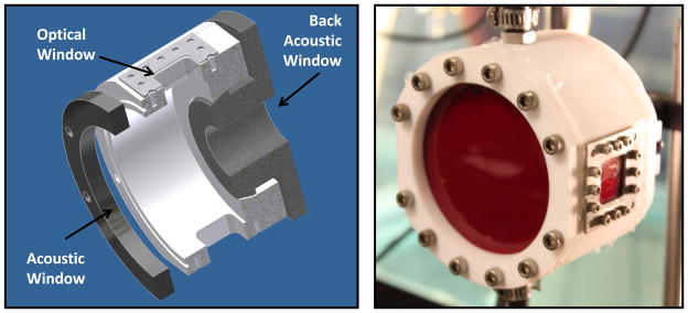
Digital solid model cross-section (left) and photograph (right) of the sample chamber used to contain materials during experiments. A large acoustic window is present in the front and a small window in the back to allow ultrasound transmission to the medium with minimal reflection. Two optical windows are positioned for backlit photography of cavitation.

Sample preparation

The cavitation thresholds of several liquid media, tissue phantoms, and canine tissue specimens were tested. Relevant acoustic and mechanical properties of the tested samples are given in Table 1. Cavitation probability vs. pressure was measured in three samples of each type. Unfiltered tap water, distilled water, and 1,3-butanediol were degassed by rigorously boiling the liquid in a 1-liter Pyrex flask on a hot plate for 10 minutes while stirring with a PTFE-coated magnetic stir bar, then sealing the flask and cooling the liquid to room temperature for the experiment before unsealing. Using this method, gas levels of ~10% O₂ saturation could be achieved, as measured in water with an O₂ meter (DO200, YSI, Yellow Springs, OH).

Table 1.

Acoustic and mechanical properties of test media at 1 MHz, taken from literature. We were not able to find viscosity data for 15% gelatin or surface tension data for solid tissues in literature.

Material	ρ (kg/m3)	c (m/s)	α (dB/cm)	η (mPa-s)	γ (mN-m)	E (kPa)
Water	998	1484	0.0022	1	72	-
Gelatin 5%	1015	1505	0.1	2	40	4.5
Gelatin 15%	1045	1550	0.1	-	40	36.0
Blood	1060	1584	0.2	3	60	-
Blood Clot	1060	1584	0.2	3	60	0.1–1.0
Kidney Tissue	1050	1560	1.0	30	-	5.7
Adipose Tissue	950	1478	0.5	12	-	1.9
1,3 Butanediol	1000	1522	0.1	97	37	-
Olive Oil	915	1440	0.2	84	36	-

^*References: Gelatin (Hiroki et al. 1991; Bot et al. 1996). Blood (Wells and Merrill 1962; Mast 2000; Rosina J 2007), Clot (Diamond 1999), Kidney (Kodama and Tomita 2000; Mast 2000; Nasseri et al. 2002), Adipose Tissue (Mast 2000; Samani et al. 2003; Geerligs et al. 2008), Butanediol (George and Sastry 2003; Chavrier 2006), Olive Oil (Halpern 1948; Treeby et al. 2009).

^†Symbols: ρ =density, c = sound speed, α = attenuation @ 1 MHz, η = dynamic viscosity, γ = surface tension, and E = elastic (Young’s) modulus.

Gelatin gel was tested as a common ultrasound tissue mimicking material that is optically transparent. Gelatin powder (G2500, Sigma Aldrich, St. Louis, MO, USA) was added to distilled water at 5% or 15% w/v. The solutions were heated in a Pyrex flask on a hot plate to boiling temperature to completely dissolve all powder, and allowed to boil for 10 minutes while stirring. The flask was then sealed until the temperature was lowered to 40°C, then added to the test chamber and allowed to cool to room temperature before the experiment.

Tissue samples were acquired from canine research subjects immediately post-mortem in an unrelated study. All protocols were approved by the University Committee for Use and Care of Animals (UCUCA). Tissue was placed in room temperature saline and experiments were conducted within 24 hours of harvest. Each sample was embedded in the chamber in 5% gelatin in the chamber, which was prepared as described above. The samples were embedded in gelatin to fix the position of the tissue relative to the chamber and displace any remaining air. All tissue samples were several cm in dimension transverse to the acoustic axis and at least 1 cm in dimension along the acoustic axis as positioned during testing.

Blood was also collected from canine research subjects and placed in a citrate-phosphate-dextrose solution (C7165, Sigma Aldrich, St. Louis, MO, USA) with a ratio of 9:1, and then stored in refrigeration at 4°C. The blood was added to the chamber directly, and allowed to return to room temperature before sealing the chamber prior to experiment. Blood clots were created from the whole blood at room temperature by addition of 0.05 mL of 0.5 M CaCl₂ per 1 mL of blood. After adding the mixture to the chamber, the chamber was placed in a water bath at 37°C for 2 hours to allow incubation of the clot. The chamber was then sealed and positioned in a degassed water tank at room temperature for the experiment.

Pressure pulse generation

A spherically-focused transducer with a center frequency of 1.1 MHz was used to generate ultrasound pulses. The focus was aligned to the center of the sample chamber in the degassed water tank. The transducer consisted of an array of eight 2-cm diameter focused elements aligned confocally with a radius of curvature of 5 cm. The overall aperture of the transducer array was 8.5 × 7 cm. The pressure distribution at the focus was ellipsoidal, and the effective -6 dB pressure beamwidth at low amplitude was 1.1 mm transverse to the acoustic axis and 6.8 mm along the acoustic axis. The multi-element transducer configuration allowed characterization of each element’s output to estimate the focal pressure beyond the cavitation threshold, as described in the following section. The transducer was connected to a class D amplifier developed in our lab (Hall and Cain 2006) through a matching network, which provided high-voltage output to each element. The amplifier signal was controlled by a field-programmable gate array (FPGA) logic board (Altera, San Jose, CA, USA). This system was used to apply a 2-cycle, sinusoidal voltage pulse to the transducer.

Due to the limited transducer bandwidth of ~50%, only the second cycle of the pulse reached the maximum amplitude, meaning that there was only one negative pressure excursion with the peak amplitude (Figure 3). This very short pulse minimized cavitation occurring through shock scattering and therefore cavitation would only be generated by the negative pressure half cycle of the incident wave. The pulse repetition frequency (PRF) for the transducer was kept very low (0.33 Hz) to minimize the possibility of cavitation from one pulse from changing the probability of cavitation on a subsequent pulse. Preliminary experiments revealed that for PRFs > ~ 1 Hz, cavitation during a pulse increased the likelihood of cavitation on the following pulse, an effect which would artificially increase the apparent probability of cavitation at a given pressure. Below this value, the probability did not change significantly with PRF in preliminary experiments.

Figure 3.

Focal waveforms at p₋ = −21.5 MPa (top) and peak negative pressure vs. transducer voltage (bottom) for the two measurement techniques used to measure large tensile pressures as well as focal measurements in water. Waveforms with the three measurements appeared nearly identical in peak negative pressure value, although the peak positive pressure was slightly reduced for the two experimental techniques. The error in peak negative pressure between measurement techniques was no greater than 15% for any pressure value, and the maximum error between the three polynomial curve fits is 11%.

In solid samples, the focus was translated for each pulse by 1 mm transverse to the acoustic propagation direction in a 10 × 10 grid for each pressure level to minimize the effects of cavitation damage to the solid sample from altering the probability of cavitation. Each focal volume in the solid received no more than one pulse at each acoustic pressure level, and only with a fraction of these did cavitation occur. One hundred pulses were applied to the sample at each pressure level tested. The pressure levels were applied in a randomized order to minimize dependency of possible hysteretic effects of pressure level on cavitation activity.

Transducer focal pressure measurement

Measurements of the focal pressure were recorded with a calibrated fiber-optic probe hydrophone (FOPH) (Parsons et al. 2006b). The FOPH was cross-calibrated by substitution comparison with two piezoelectric reference hydrophones (HGL-0085 and HGL-0200, Onda Corporation, Sunnyvale, CA, USA). Each hydrophone had a reported calibration uncertainty at 1.1 MHz of ± 1 dB (~ ± 12%), thus the sensitivity was taken from the average of both measurements with uncertainty $\epsilon /\sqrt{n}=\pm 8.5\%$. Both reference hydrophones’ measurements were in agreement (at measured pressures up to 3 MPa) within 4%. The measurements were captured in a free-field condition in water degassed to 25% O₂. Pressure levels up to 23 MPa peak negative pressure could be recorded in water with the FOPH. Above this level, cavitation often occurred on the hydrophone or the fiber tip fractured, which precluded further measurements. Two separate indirect measurement techniques were employed to determine the peak negative pressure at the focus vs. transducer driving voltage beyond the measureable range in water.

For the first technique, the fiber optic hydrophone was positioned in another liquid which was found to have a higher threshold for cavitation: 1,3 butanediol. This method has been used with piezoelectric hydrophones in castor oil to prevent cavitation damage to their surface from lithotripter shockwaves (Howard and Sturtevant 1997). Butanediol has a room temperature density (ρ = 1005 kg/m³) and sound speed (c = 1505 m/s) very similar to water (ρ = 998 kg/m³ and c = 1484 m/s), minimizing acoustic reflection at the interface between the two. The fiber probe was positioned in a small container of butanediol with an acoustic window of 12-μm low-density polyethylene facing the transducer. To ensure the attenuation in butanediol did not alter the measurement significantly, the probe tip was positioned only 5 mm from the interface. The sensitivity of the fiber optic hydrophone in butanediol was calculated by comparison of the focal pressures measured in water with the FOPH and piezoelectric hydrophones at low pressure values.

The second technique used to estimate the focal pressure was summation of measurements from individual elements’ pressure output at the focus. Each of the 8 elements in the transducers was driven separately, and the pressure waveforms were measured at the transducer focus in degassed water with the fiber optic hydrophone. The waveforms from each element for a given driving voltage were then summed to estimate the pressure waveform generated by the transducer when all 8 elements are driven in phase. Generally, this technique is not acceptable for high-amplitude measurements, because nonlinear propagation is dependent on the pressure amplitude along the path from the transducer to focus. When an element is driven individually, the pressure in and around the focus is lower, meaning the waveforms measured independently will be less distorted than the waveform with all elements driven simultaneously. This effect can lead to significant errors in peak pressure levels. In this study, however, the elements are each focused individually and the beam paths from each element do not overlap except at the transducer focus, which is only a few mm distance. Thus, most of the nonlinear distortion is expected to develop in the nearfield of each element, independent of the others. This argument was verified by comparing the measurements at lower pressures with focal waveforms captured with all 8 transducer elements driven at the same time. The pressure calibration results from each method are shown in Figure 3.

With the FOPH in butanediol, the pressure measurement error compared with the standard measurement in water up to supply voltage = 230 V (p₋ = 23 MPa) was ε ≤ 10%, and ε_mean = 2.6%. Using the method of element summation to predict the focal pressure, the error compared with the standard measurement was ε ≤ 15%, and ε_mean = 8.7%. At higher transducer output where the standard measurement could not be made in water, the two methods agreed within 15% of each other for all measurements. Based on the better agreement of the data in water and butanediol, the data in butanediol were fit to a 5^th order polynomial which was used to determine the peak negative pressure vs. voltage. The overall uncertainty for the absolute value of peak negative pressure is estimated to be ± 8.9% based on the combined uncertainty of the reference hydrophone and comparison between water and butanediol measurements. Corrections were also made to the focal pressure amplitudes for sample attenuation and reflection based on literature values for acoustic impedance and absorption, assuming linear propagation. These corrections were < 0.9 dB for all samples.

Camera measurement and image processing

A high speed camera (V210, Vision Research, Wayne, NJ, USA) was used to capture images of the focal zone directly after the propagation of each pulse through the focus in all transparent media. The camera was focused with a macro-bellows lens (Tominon, Kyocera, Kyoto, Japan) through the optical window of the chamber to observe the focal region. The camera was backlit by a continuous light source to produce shadowgraphic images of cavitation bubbles. The camera was triggered to record one image for each pulse applied, 3 μs after the beginning of the pulse reached the focal center. This timing coincided with the largest negative pressure excursion of the pulse reaching the far −6dB pressure point of the focus. This ensured that the pressure pulse had passed over the entire focal volume at the time of capture. The camera exposure time was 2 μs for all images.

After acquisition, images were converted from grayscale to binary by an intensity threshold determined by the background intensity of the shadowgraphs in image processing software (MATLAB, The MathWorks, Natick, MA, USA). Bubbles were indicated as any black regions > 5 pixels. The minimum resolvable diameter of a bubble was about 15 μm, due to the magnification of the described experimental arrangement and minimum 5-pixel area. The number of frames which contained detected cavitation bubbles on an image was recorded and the fraction of total frames for which any cavitation was detected was recorded as the cavitation probability.

PCD measurements and signal processing

While high-speed photography simplifies detection of cavitation in transparent media, it cannot be used with most tissue samples. Additionally, the camera only detects the presence of cavitation at one time point, and does not provide information regarding the cavitation dynamics. An acoustic method was also used to identify cavitation in the focal zone in all media. A passive cavitation detector (PCD) using a high-bandwidth 5-MHz focused transducer with focal length = 10 cm was positioned behind the therapy transducer with their foci overlapping. The central hole in the therapy transducer provided an unobstructed aperture for the PCD. The PCD was connected to a signal amplifier (PR5072, Panametrics NDT, Waltham, MA, USA), which was in turn connected to an oscilloscope (LT372, Lecroy, Chestnut Ridge, NY, USA). The time window was selected to record the backscatter of the pressure pulse from cavitation bubbles (Roy 1990; Herbert et al. 2006), as well as emissions from bubble collapse well after the pulse passed the focus (Bailey et al. 2005; Brujan and et al. 2005).

To determine whether cavitation occurred during a pulse, the signal generated by backscattering of the incident pulse from the focus was analyzed. A significant fraction of the incident wave energy is scattered when a cavitation bubble expands, greatly increasing the backscattered pressure amplitude received by the PCD. This signal appeared on the PCD at the time point corresponding with the time of flight between the focal lengths of both transducers. Since the walls of the chamber were at least 1.5 cm from the focus, the possibility of the scattering from other sources besides cavitation could be minimized by time windowing the signal. The integrated frequency power spectrum of the backscatter signal β(t) was used as a measure of whether cavitation occurred during the pulse. The signal’s Fourier transform, B(f), was first calculated, and the integrated power spectrum, S, was calculated by

$$S=\sum _{f_1}^{f_2}{\mid B(f)\mid }^2.$$ (1)

It is common to evaluate subharmonic or superharmonic broadband emissions which are generated solely by cavitation under lower-amplitude long-burst excitation, when these frequencies are not present in the incident pressure waveform (Chen et al. 2003; Rabkin et al. 2005). However, the pulse applied in this study was broadband because of the many harmonics from nonlinear distortion and short pulse duration. The largest component of the backscatter was near the center frequency (1.1 MHz), and thus the power spectrum of the backscatter signal around this frequency (0.6 – 1.6 MHz) was used as a measure of cavitation presence rather than the high-frequency broadband spectrum.

The threshold for S for a cavitation event was determined by scaling the expected value for S based on the focal pressure curve obtained from calibration measurements. The following procedure was applied:

1. The integrated power spectrum, S_F, for each of the focal pressure waveforms recorded by fiber optic hydrophone was calculated using Eq. 1.

2. The integrated power spectrum, S_PCD, for the pressure signals received by the PCD was calculated. The mean and standard deviation of S_PCD for 100 pulses were calculated.

3. It is reasonable to expect that the backscatter intensity will increase in proportion with focal intensity when cavitation does not occur, and a plot of S_PCD vs. S_F at low pressures would follow a linear relationship. The expected value of S_PCD vs. S_F is given by:

   $$S_{\mathit{PCD}}(V_n)=\frac{S_F(V_n)}{S_F(V_{n-1})}·S_{\mathit{PCD}}(V_{n-1}).$$ (2)

   If, for a single pulse at a voltage V_n, the value S_PCD exceeds the expected value given in Eq. 2 by 5 standard deviations, it is considered that inertial cavitation has occurred. The voltage V_n−1 is then chosen as the last point for the linear fit.

4. The means and standard deviations for S_PCD(V_n, V_n+1,…,V_N) are estimated by a least-squares linear regression to the values S_PCD(V₁, V₂, …,V_n−1) and linear extrapolation with respect to S_F.

5. For each of the signals recorded by PCD for (V_n, V_n+1, …, V_N), the value S_PCD is compared with the expected value calculated in step 4. If this value is greater than expected by 5 standard deviations, then inertial cavitation is considered to have occurred during the pulse.

This method allowed a quantitative definition for whether a signal was above the threshold for cavitation, based on whether the backscattered signal was ‘much larger’ than expected by the relationship between S_PCD and S_F. It is assumed that cavitation did not occur at the lowest pressure values tested that a linear relationship for backscatter vs. focal pressure can be established. At least 5 pressure levels starting at 1.3 MPa were measured where the relationship was found to be linear as determined by step 3 in each sample, and no signals or images suggested that cavitation occurred. The assumption of a linear extrapolation with respect to S_F was also verified in water at higher amplitudes by extracting the mean value of S_PCD for pulses where inertial cavitation was not detected by high-speed photography as outlined above.

We have estimated the sensitivity of the method outlined in this section by producing cavitation in a sample of distilled water artificially nucleated with 1 μm PTFE particles in high concentration. In this sample, cavitation could be detected with good accuracy down to p₋ ~ 5 MPa. It is important to note that this method is less sensitive than techniques using detection of broadband emissions. However, as is demonstrated in the results, cavitation was very rarely observed in the range of 5–15 MPa, thus it is expected inertial cavitation would occur with even lower probability for p₋ < 5 MPa. By the same experiment, the optical technique was able to identify cavitation as low as p₋ = 3.1 MPa, and the results gave good agreement between the two detection techniques at greater pressure amplitudes.

The PCD signal also indicated violent bubble collapse from inertial cavitation based on a secondary emission recorded at a later time than the backscatter signal (Figure 4). This signal consisted of a short, positive pressure spike created by inertial collapse of the bubble. This signal has been characterized in previous research using passive cavitation detectors or hydrophones to measure the bubble collapse pressure (Bailey et al. 2005; Brujan and et al. 2005; Chitnis 2006). The collapse time could be characterized by the time difference between the start of the backscatter signal and the collapse signals.

Figure 4.

Sample PCD temporal signals (left), corresponding windowed and normalized frequency domain amplitude spectra (center), and corresponding camera photographs (right) of cavitation at the transducer focus. The PCD signals show an initial burst near the therapy frequency due to backscatter from the cavitation bubbles, as well as one or more short positive spikes – shockwaves from cavitation collapse. A small signal around 30 μs is caused by a reflection of the therapy pulse from the back membrane of the housing, and is windowed out of the signal when evaluating cavitation with the PCD. Ultrasound propagation in the photographs is from right to left.

Theory

A single bubble cavitation model was implemented to evaluate the pressure threshold response of cavitation nuclei related to the measured pressures at which cavitation was observed. Since the primary focus of this study is the initial threshold behavior and expansion phase of the bubble, a simple model was used which does not account for extreme conditions under bubble collapse, although accounts for liquid compressibility. The Keller-Miksis equation (Keller 1980), modified by Yang and Church to include elasticity (Yang and Church 2005), was used to describe the radius-time behavior of cavitation bubbles in a viscoelastic medium, given as

$$\left(1-\frac{\stackrel{.}{R}}{c}\right)R\ddot{R}+\left(1-\frac{\stackrel{.}{R}}{3c}\right)\frac{3}{2}{\stackrel{.}{R}}^2=\left(1+\frac{\stackrel{.}{R}}{c}\right)\frac{p_w(\stackrel{.}{R},R,t)}{\rho }+\frac{R}{\rho c}\frac{\partial p_w}{\partial t},$$ (3)

where R is bubble radius, the dot is a time derivative, c is the speed of sound in the medium, and ρ is the medium density. p_w is the pressure at the bubble wall in the liquid, which includes terms for the internal gas pressure in the bubble following adiabatic conditions, as well as pressure due to surface tension, viscosity, elasticity, and acoustic pressure,

$$p_w(\stackrel{.}{R},R,t)=\left(p_0-p_v+\frac{2\gamma }{R_0}\right){\left(\frac{R_0}{R}\right)}^{3\kappa }-p_0-\frac{2\gamma }{R}-\frac{4G}{3R^3}(R^3-{R_0}^3)-\frac{4\eta \stackrel{.}{R}}{R}-p_a(t).$$ (4)

In Eq. 4, p₀ is the ambient pressure far from the bubble wall in the liquid, p_v is the vapor pressure in the bubble, γ is the surface tension of the liquid, R₀ is the initial bubble radius at time t = 0, κ is the polytropic index (ratio of specific heats), G is the shear modulus, η is dynamic viscosity, and p_a(t) is the time-varying acoustic pressure applied to the bubble. To numerically simulate the bubble response, the initial conditions for pressure were first found by Eq. 4. Next, the bubble radius vs. time is found by Eq. 3 using a variable order solver based on numerical differentiation formulas (ode15s, MATLAB, The MathWorks, Natick, MA, USA).

A nonlinear pulse model with a Gaussian pulse envelope was used to simulate the pressure waveform (Ayme and Carstensen 1989). This pressure pulse is given as

$$p_a(t)=p_f\sum _{m=1}^{\infty }\left[\frac{sin(m\omega (t-\tau )+\phi )}{m}\right]·exp\left[-{\left(\frac{t-\delta }{\xi }\right)}^2\right],$$ (5)

where p_f is the fundamental pressure amplitude, ω is the frequency, τ is the initial phase of the wave so p_a(0) = 0, ϕ is a phase shift to create proper waveform asymmetry, δ is the time delay to the center of the pulse, and ξ defines the pulse width. For the simulation at 1.1 MHz, ω = 6.9 × 10⁶ rad/s, τ = 1.25 π/ω, ϕ = −π/4, δ = 2.85 μs, and ξ = 1.2 μs. The infinite sum was truncated to m = 100. This gave a pulse which closely approximated the shape and ratio p₊/p₋ of the waveform displayed in Figure 3.

Results

Cavitation probability in water

Cavitation bubbles were observed on high speed camera in an increasingly larger area with pressure when a certain negative pressure was exceeded (Figure 4). The probability of observing cavitation in the focal volume followed a sigmoid function, given by

$$P(p_{-})=\frac{1}{2}\left[1+\mathit{erf}\left(\frac{p_{-}-p_t}{\sqrt{2{\sigma }^2}}\right)\right],$$ (6)

where erf is the error function, p_t is the pressure at which the probability P_cav = 0.5. σ is a variable related to the width of the transition between P_cav = 0 and P_cav = 1, with ± σ giving the difference in pressure from about P_cav = 0.15 to P_cav = 0.85 for the fit. The values for p_t in distilled, degassed water were found to between p_t = 26.9 MPa – 28.1 MPa, with σ = 0.8 – 1.7 MPa. Note that at lower amplitudes, cavitation was occasionally observed which deviated from the curve function. The lowest peak negative pressure amplitude at which cavitation was detected (p_min) in any of the 3 distilled water samples was 17.7 MPa. These cavitation events were likely due to contamination of the sample by heterogeneities in the liquid, which could not be entirely avoided throughout the experiment. In the experimental data, cavitation was observed with P_cav = 1 for p₋ > −30 MPa. As P_cav approaches 1, multiple cavitation bubbles were observed by high-speed photography each pulse within the focal region. The bubbles’ diameters were consistent between pulses at the time point captured by the camera.

The PCD detected a distinct signal in the presence of single or multiple cavitation events. First, a multicycle burst with a center frequency near 1.1 MHz was detected with a time delay corresponding to the time for the therapy pulse to travel from the transducer to the focus to the PCD - between 100 – 110 μs from the time the test pulse was emitted. Between 10 – 100 μs after this burst signal was received, one or more short positive pressure spikes were observed on the PCD signal, indicating shocks emitted during bubble collapse (Brujan et al. 2005). When no cavitation was observed on high-speed camera, the scattered signal was small and collapse signals were absent (Figure 4). The accuracy of detection was validated in the set of data for water. Figure 5 shows an example of the relative values of S_PCD vs. pulse number for 100 pulses near the cavitation pressure threshold p_t in degassed, distilled water. Overall, the error rate was ≤ 2% for a data set at one pressure level. These errors in detection often occurred when a cavitation bubble outside the focus was present at lower pressure levels.

Figure 5.

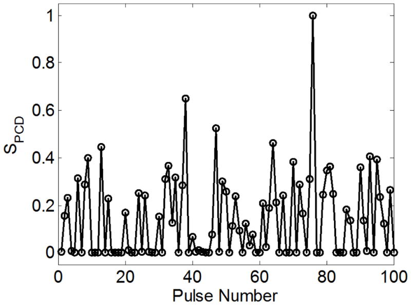
Integrated power spectrum (S_PCD) for the signal in distilled water vs. pulse number for 100 pulses. The peak negative pressure for this data set was p₋ = 28.6 MPa - near the 50% threshold for cavitation. A bimodal distribution of values is evident, with the lower, more consistent values indicating absence of cavitation, and the larger, more variable values indicating the presence of one or more bubbles.

Purity and gas concentration of the water sample had a small effect on the cavitation threshold probability curve. In unfiltered tap water, which was only mildly degassed to 90% O₂ concentration, p_t varied from 26.0 – 26.4 MPa and σ = 1.4 MPa for all 3 samples, slightly lower than the mean value p_t for distilled water with about 10% O₂ concentration. Additionally, p_min was 13.5 MPa, lower than distilled water.

Cavitation probability in different samples

A similar function of cavitation probability vs. pressure was observed in all water-based media (Figure 6). Additionally, p_t was similar in these materials. The fit curves for the experimental cavitation probability data in tissue mimicking materials of 5% and 15% gelatin in distilled water gave p_t = 26.5–27.8 MPa and p_t = 26.4–29.4 MPa respectively. One difference between these samples was that the bubbles were generally smaller in size at the time point captured by the camera for the 15% gelatin than the 5% gelatin or water (Figure 7). However, the region over which cavitation occurred in each sample was similar at similar pressure levels. While the initial backscatter signal was detected in both samples, bubble collapse shockwaves were undetectable in almost all signals in 15% gelatin, while at a similar pressure level, they were observed every pulse in 5% gelatin and water.

Figure 6.

Example probability data and fit curves for each sample type tested. Each data point is the fraction of 100 pulses where cavitation was detected. Curves were fit by nonlinear least-squares regression to each data set.

Figure 7.

Example PCD signals (left) and corresponding high-speed photographs (right) of cavitation in distilled water and gelatin at 5 and 15% concentrations. The black arrows indicate bubble collapse shockwave signals received by the PCD. Note that the diameters of the bubbles in 15% gelatin are significantly reduced compared with the other two samples, although the cavitation is observed over the same volume within the focus. Ultrasound propagation in these images is from right to left.

A similar threshold was also observed in canine blood, clotted blood, and kidney. In these materials, no images could be captured by the camera, but the same cavitation backscatter signals and bubble collapse signals were observed in all three materials. Measurements in blood and blood clot indicated p_t = 26.5–27.6 and 26.7–26.9 MPa, respectively. Kidney tissue was slightly higher with p_t = 28.2–30.0 MPa. The value σ was similar to those above, as were the values p_min = 16.8 MPa for blood, 14.4 MPa for clot, and 16.1 MPa for kidney.

There was a larger variance in threshold for the three materials which were not primarily water-based: 1,3 butanediol, olive oil, and canine visceral adipose tissue. The threshold in butanediol (p_t = 34.9 – 35.6) and olive oil (p_t > 36) were greater than any of the water-based samples. In olive oil, the curve could not be properly fit to a threshold because the probability of cavitation was low even at the maximum pressure output from the transducer. However, it is assumed that P approaches 1 at pressures much greater than the range in this study for both of these materials, similar to other media. Bubble activity was also suppressed in butanediol and olive oil; cavitation bubbles appeared similar size to those in 15% gelatin and cavitation collapse shockwaves were not visible on PCD signals. The threshold in visceral adipose was significantly lower than in any of the above media, with p_t = 13.7 – 16.9 MPa, and σ = 0.5 – 0.8.

Example probability curves for different materials are given in Figure 6, and a summary of the results of all samples is given as Table 2. The fit curves were analyzed statistically to determine if the difference in the values p_t were significantly different from each other. The standard errors for the parameters p_t were estimated by a covariance matrix using the delta method (Hosmer and Lemeshow 1992). The curves were compared using a two-sample t-test with statistic $t\left(p_{t1}-p_{t2},\sqrt{{{SE}_1}^2+{{SE}_2}^2}\right)$ at a 95% confidence interval. Note that the standard error does not include the uncertainty in absolute pressure from the hydrophone measurement, only the uncertainty in the fit, because the values p_t are relative. In general, the standard errors in the estimate of p_t were small (~0.1 – 0.2 MPa) compared to the variance between samples of the same type. With the exception of clot, a pair of samples existed within one sample type with a statistically-significant difference (p-value < 0.05). Additionally, there existed at least one pair between any two sample types with a significant difference. Thus, although p_t values were similar in many cases, there appeared small but measureable differences between these samples.

Table 2.

Values for the peak negative pressure p_t at which a fit curve set P_cav = 0.5 for each of the samples, the mean values for p_t and s, and the minimum pressure level at which cavitation was detected in the sample type, p_min. All values are pressure in MPa. The cavitation threshold in olive oil could not be determined since the transducer could not generate large enough pressure amplitude to cause cavitation with high probability.

Material	pt (1)	pt (2)	pt (3)	pt (mean)	σ (mean)	pmin
Water (Dist. 10% O2)	28.1	26.9	27.2	27.4	1.3	17.7
Water (Unfilt. 90% O2)	26.4	26.2	26	26.2	1.4	13.5
Gelatin (5%)	26.5	27.8	27.7	27.3	1.3	17.2
Gelatin (15%)	26.4	29.4	28.2	28	0.8	15.6
Blood	27.6	26.7	26.5	26.9	1.3	16.8
Blood Clot	26.7	26.9	26.8	26.8	1.2	14.4
Kidney Tissue	30	29.9	28.2	29.4	1.1	16.1
Adipose Tissue	15.6	16.9	13.7	15.4	0.6	9.8
1,3 Butanediol	35.6	34.9	35.2	35.2	1.6	27.9
Olive Oil	>36	>36	>36	>36	-	23.2

Simulated Bubble Behavior

The threshold in water was used to determine the radius of a model bubble nucleus which has a pressure threshold for inertial cavitation p_t. Simulating a single spherical gas nucleus in water, the bubble radius and peak negative pressure of the applied pulse were varied to evaluate the bubble response. Bubbles expansion was minimal (R_max < 2 R₀) below a certain value for p₋, while above this value, large bubble growth and collapse were observed (R_max > 10⁴ R₀). The peak negative pressure corresponding to this transition was defined as the threshold for inertial cavitation. To achieve this threshold near p₋ = 28.1 MPa (similar to water-based samples), the necessary initial bubble radius was ~2.5 nm. The threshold was very distinct in water; a change in the applied p₋ of 1 kPa caused a change in R_max from 4.2 nm to 30 μm (Figure 8). This characteristic is not observed for micron-sized nuclei in response to ultrasound pulses, which undergo a less well-defined transition period between small linear oscillation and large inertia-dominated bubble growth and collapse (Leighton 1994).

Figure 8.

Simulated maximum bubble radius achieved in response to a 2-cycle pulse vs. peak negative pressure of the pulse for a 2.5 nm initial radius. A nucleus of this size has a distinct threshold for inertial cavitation, in this case near p₋ = 28.2 MPa.

The nuclei in this situation are much smaller than the corresponding resonant diameter for a 1.1 MHz wave. Because of the small size of the nucleus in water, the cavitation threshold was nearly independent of frequency in the range of interest for ultrasound therapy (28.1 MPa at 0.1 MHz vs. 28.4 MPa at 10 MHz). The pressure threshold for bubbles this size is strongly dominated by surface tension of the medium in the simulation. Despite the differences in measured surface tension of the tissues and tissue phantoms from pure water, their p_t values were similar, suggesting possibly either the radius of the model nucleus should be considered different between them, or the surface tension on the nanometer scale may be similar to water. Butanediol, which does not contain water, has a surface tension is 37 mN/m and the viscosity is 97 mPa-s. The bubble radius that fits the threshold of 35.6 MPa is 1.1 nm.

Other mechanical properties had a minimal effect of the threshold at 1.1 MHz. However, increasing viscosity created a stronger frequency-dependency for the threshold (Figure 9), a trend similar to that shown by Allen et al (1997). At 0.1 MHz, the threshold is 28.1–28.3 MPa for η = 0.001–0.1 Pa-s. Increased viscosity produced smaller values of R_max, but did not change the threshold significantly. Change in the elasticity in the range G = 0 – 100 kPa (the range for soft tissues) also did not significantly affect the threshold (Figure 9), nor the maximum radius of the bubble. These data from the model support photographic observations in the gelatin phantoms which suggested that the threshold does not change significantly due to these properties, although the growth and dynamic behavior of bubbles was suppressed.

Figure 9.

Simulated cavitation threshold pressure for a 2.5-nm radius bubble vs. viscosity (top) and elasticity (bottom) for 2-cycle pulses with center frequencies of 0.1, 1.1, and 10 MHz.

Superthreshold cavitation behavior

When the applied pressure amplitude was near p_t, single cavitation bubbles appeared primarily in a region at the center of the focal zone. When the focal pressure was significantly in excess of p_t, multiple cavitation bubbles occupied a region similar in shape to the focal zone each pulse. By integrating the 100 binary images of the cavitation observed by the camera at a given pressure level, the total region within the frame where cavitation was observed could be analyzed. This provides some indication for histotripsy of the region over which cavitation damage would be expected to occur (Maxwell et al. 2010b). Figure 10 shows the integrated cavitation maps for water and 15% gelatin. Note that the extent of the bubble locations is similar at the same p₋, but the extent of the total cavitated region is smaller because of the suppressed bubble expansion in gelatin.

Figure 10.

Integrated images of the locations where cavitation occurred over 100 pulses, shown in white for two materials with similar thresholds. Over several pulses, the positions of cavitation add to generate a pattern similar to the focal zone of the transducer. Ultrasound propagation in these images is from right to left.

Assuming one has accurate knowledge of the peak pressure focal distribution, cavitation probability vs. pressure, and the cavitation dynamics, it may be possible to predict the extent of cavitation as a result of a finite number of ultrasound pulses with a given p₋. First, the peak negative pressure vs. position can be mapped for a transducer from hydrophone measurements. Although the focusing is altered for a pulse which is distorted by nonlinear propagation, the beam profile for the peak negative pressure is similar to that in a linear simulation (Canney et al. 2008). Next, the peak radius of a bubble vs. pressure can be determined by a simulation similar to that described above. Finally, the curves given in Figure 6 can be used to determine the probability of cavitation P(x,z) as a function of pressure level p₋ (x,z). Due to the finite size of the area tested in the experiments above, however, the probabilities recorded are for the entire focal zone. Thus, P must be normalized to the volume of the focal zone. A Monte-Carlo-type simulation may then performed, where the probability P(x,z) is compared with a random value between 0 and 1 at each spatial point for each pulse. Cavitation then occurs at point x,z for pulse n if the probability value is greater than a random number between 0 and 1 (i.e. P_norm (x, z) > rand (x, z)). This simulation then predicts the cavitation field for each pulse. is Pnorm obtained by multiplying P by a coefficient, determined by matching the simulation to the experiment such that the probability of cavitation occurring anywhere in the field of the simulation for 1 pulse is ~0.5 when p₋ = p_t. Figure 11 shows an example of the total cavitated region from the simulation for different peak negative pressures, as well as the corresponding experimentally observed cavitated regions. Figure 12 gives the measured axial and lateral dimensions of the cavitated regions from simulation vs. p₋. Good agreement is seen for the axial dimension, although the transverse dimension was somewhat smaller for simulation than in the experiment for high pressure amplitudes.

Figure 11.

(Left) Integrated 2D cavitation map for n = 100 pulses resulting from a Monte-Carlo simulation using the probability curve, pressure map, and peak bubble radius for different peak negative pressures in unfiltered water (p₋ = 26.4 MPa, σ = 1.3 MPa). (Right) Binary image of the experimentally observed cavitation by high speed camera, integrated over n = 100 pulses for the same focal pressure levels in unfiltered water.

Figure 12.

Dimensions of the cavitation regions vs. peak negative pressure for simulation and experiment in unfiltered water. (Top) Axial dimension of the cavitation zone (excluding bubbles outside the focus for experimental measurements). (Bottom) Measured and simulated transverse dimension of the cavitation region at the focus.

Discussion

In this study, we measured the peak negative pressure necessary to consistently achieve inertial cavitation in response to a single, microsecond-length pulse in multiple tissues and tissue-mimicking media. A similar pressure threshold has been observed specifically in water in several past investigations by other groups applying quasi-static tension (Briggs 1950), high-amplitude shock waves (Wurster et al. 1995; Sankin and Teslenko 2003) or acoustic pulses (Herbert et al. 2006), and the pressure values reported (24 – 33 MPa) are among the greatest measured for cavitation thresholds in water, with the exception of work in quartz inclusions (Zheng Q et al. 1991). Perhaps the most thorough work on this has been reported by Herbert et al (2006), who used a similar acoustic method to apply 1 MHz 4-cycle pulses to a purified water sample. The authors found a peak negative pressure threshold near 25 MPa, although the reported values vary slightly for different methods of pressure measurement between 24 – 28 MPa at 20°C (Herbert et al. 2006; Arvengas et al. 2011). The cavitation probability followed an asymmetric sigmoid curve trend with similar width to our measurements. Their results also indicated that the statistical threshold was independent of the purity to some degree by introducing particles into the water sample. While cavitation was occasionally observed at lower pressures, the higher probabilities (P_cav > 0.1) were not observed until p₋ > 20 MPa. Measurements recorded for the present study indicated only a minor variation in threshold between water samples (p_t,mean = 27.4 vs. 26.2 MPa), also in agreement with the data reported by Herbert et al.

This threshold was similar in all materials which were primarily water-based (water, gelatin, blood, clot, and kidney), despite the variety of other species within these samples. Less data is available regarding cavitation in such tissues compared with water. However, recent measurements have detected broadband noise indicative of inertial cavitation in ex-vivo liver near p₋ = 2 MPa under 4 second continuous exposures (McLaughlan et al. 2010). While we did not measure cavitation at such low values, this is likely due to the limited statistics collected in our study and much shorter exposure duration. We applied only ~200 cycles per pressure level per sample, while the values in MacLaughlan et al. are the lowest pressure amplitude at which cavitation was detected over several million acoustics cycles. Additional effects, such as heating and rectified diffusion can become prominent over such exposures and may alter the medium or nuclei population. While it is likely cavitation occurs at such low pressures, the probability of its detection during a single short pulse may be very low, given that we did not observe cavitation until p₋= 9.8 MPa with 100 pulses in any of the samples. Gateau et al (2011) have also recently explored cavitation probability in sheep’s brain in-vivo, using focused 2-cycle 660kHz pulses similar to those employed in our study. The authors applied a pulse train with p₋ as great as 22.4 MPa, and determined the probability for cavitation formed at the focal position in the brain. The lowest pressure amplitude at which cavitation was detected in over 120 positions was p₋ = 12.7 MPa, close to the minimum values in our study. Interestingly, the authors found that cavitation was detected with a probability near 1 after 25 pulses were applied at p₋ = 22.4 MPa. It is possible that the larger volume of the focus, lower frequency, or faster pulse repetition in this study required a lower pressure amplitude to achieve cavitation with greater probability. We intend to explore such variables in future work.

In the present work, no discernible trend was found between water content and threshold or other bulk properties of the media such as viscosity, elasticity, surface tension, or acoustic impedance. The water content of most samples ranged from ~65% – 100% based on literature (Forbes et al. 1953; Keitel et al. 1955; Kiricuta and Simpleceanu 1975). While the macroscopic properties of these samples vary significantly, these values may not be relevant for cavitation nuclei at the nanometer scale. In the nanoscopic range, tissues are an extremely diverse combination of molecules and almost certainly vary from position to position within the structure. Unfortunately, it was not possible to discern in this study whether cavitation was preferentially located within specific cellular or structural regions of tissue. There was, however, some difference in p_t between the sample types. Differences in acoustic attenuation and reflection may have contributed to unequal pressure levels at the focus for a given applied voltage to the transducer. Based on literature values, the maximum attenuation was no more than 0.5 dB in any tissue sample. The maximum difference in acoustic impedance with water gives a reflection coefficient at the water/sample interface of < 0.06. Both of these effects were taken into account in the focal pressure estimation, thus the error in pressure estimation because of acoustic mismatch and attenuation is likely small. Possibly, the threshold differences may have occurred because of the necessarily different preparation methods of the samples, which resulted in unequal gas concentration. Despite this minor variation, the presence of water appeared to be the strongest predictor of the cavitation threshold.

Materials which were not primarily water-based had much greater discrepancy in p_t compared with those described above. Butanediol is a hydroscopic liquid with similar acoustic properties to water, but a higher viscosity. This material has been proposed as a potential tissue mimicking material for ultrasound studies (Granz 1994). The higher threshold in this material and the similarity of acoustic properties to water allowed us to record pressure measurements with p₋ > 30 MPa, a technique which was validated by comparison with measurements in water at lower pressure levels. Canine visceral adipose tissue was found to have a p_t ~ 15 MPa. Triglycerides constitute about 80% of adipose tissue (composed of ~47% oleic acid, 24% palmitic acid, 15% linoleic acid, 14% others) and about 20% water (Forbes et al. 1953; Malcom et al. 1989). While this result suggested that perhaps these substances contain a lower cavitation threshold, olive oil which is nearly 100% triglycerides (composed of ~70% oleic acid, 13% palmitic acid, 10% linoleic acid, and 7% others) had a considerably higher threshold than either water or fat. It is likely that the lipid/water interfaces are in fact the weak points in the structure due to the low interfacial tension. For instance, the surface tension at an olive oil/water interface is 23.6 mN/m, lower than either of the two constituents (Fisher et al. 1985). Couzens and Trevena (Couzens and Trevena 1974) noted in a previous study involving oil/water interfaces that the cavitation threshold was lower at the interface than in either of the bulk media. Similarly, we suspect that adipose tissue is more susceptible to cavitation because of its inhomogeneous emulsion of lipids and water. Although not reported in the results, we have also tested canine skeletal muscle using the same methods described in this paper. The cavitation probability was highly dependent on the focal position of the tissue, likely because of the intramuscular fat throughout the structure. However, the pressure range for cavitation was bracketed by those for adipose tissue and water.

Numerical simulation of the bubble dynamics suggested that a model bubble nucleus of 2.5 nm would have a pressure threshold of ~28.2 MPa in water. For nuclei in this size range, surface tension is the dominant force controlling the threshold by the Laplace pressure. In this respect, it is similar to the Blake threshold (Leighton 1994). In the frequency range of interest for therapy (0.1 – 10 MHz), the threshold was nearly independent of frequency for elasticities and viscosities reported for tissues (Wells and Merrill 1962; Diamond 1999; Kodama and Tomita 2000; Nasseri et al. 2002; Samani et al. 2003; Geerligs et al. 2008), although a greater dependence on viscosity was predicted for higher frequencies. Note that while the threshold of an individual nucleus may not be a strong function of frequency, the probability of cavitation also depends on the number of nuclei within the focal volume. As such, if an equivalent transducer with a higher frequency were applied, one would expect an increase in the predicted pressure threshold due to the smaller volume of the focus. This is supported by data from Arvengas et al. (2011), who compared the cavitation statistics for 1 and 2 MHz transducers in distilled water and found an incremental increase in threshold at 2 MHz by a factor of ~1.3. Additionally, the true nuclei population in water appears to be a distribution of radii ≤ 2.5 nm rather than a single value with a set threshold. This is evident by the significantly greater number of cavitation bubbles activated in Figure 1 compared to Figure 7 within a volume. Theoretically, shock scattering can produce tensile pressure as great as the peak-peak values of the incident wave, which in the case shown in Figure 1 gives p₋ > 100 MPa. It appears that a greater negative pressure excursion will activate additional smaller nuclei coexisting with those which cavitate near p_t.

In histotripsy, it is known that specific tissues are more resistant to cavitation and mechanical tissue damage (Cooper et al. 2004). Rather than their intrinsic threshold for cavitation being different however, the results here suggest that bubble expansion is suppressed. As shown in Figure 10, cavitation in the gelatin with higher concentration had a similar threshold to water, but the individual bubbles presumably did not grow to as large of radii as those in water. Thus, while the macroscopic properties appeared to have minimal effect on the threshold, they did alter the bubble behavior. Not only might this reduced activity result in minimal tissue damage directly, but it may also suppress the shock-scattering mechanism of forming cavitation clouds. Smaller bubbles will not cause sufficient scattering to initiate this action, and no cavitation cloud would be formed in the tissue. However, as suggested by Freund (2008), cavitation dynamics may change over several thousand acoustic pulses as cyclic growth and collapse of the same cavitation bubbles damage the surrounding tissue, reducing the local effective viscosity and elasticity of the tissue and progressing mechanical tissue damage.

With knowledge of the cavitation dynamics, the pressure thresholds, and the beam pressure profiles for the transducer, it may be possible to create a more predictive mechanical ultrasound therapy with cavitation. It is difficult to determine the location of heterogeneous nuclei before treatment, and this can lead to clouds forming in distinct locations along the propagation axis of the focal zone while other locations remain completely uncavitated in histotripsy (Maxwell et al. 2011). In contrast, the 2-cycle pulse used in this study appeared to generate cavitation more uniformly within the focal zone. Furthermore, the location and extent of the cavitation observed on high speed camera was in good agreement with a stochastic model of this cavitation activity based on the experimental pressure thresholds. A more sophisticated estimate of the number of nucleation sites per unit volume or the full nuclei distribution would significantly enhance such a model, as would a more thorough coupling of bubble dynamics simulation with pressure waveforms spatially. While cavitation has often been regarded as unpredictable in ultrasound therapy, this short-pulse strategy could create a controllable modality, assuming such cavitation can cause the necessary mechanical tissue ablation efficiently.

Conclusions

In this study, the probability of inertial cavitation occurring during a single, 2 cycle, 1.1 MHz focused ultrasound pulse was measured in several media relevant to focused ultrasound therapy. Cavitation was formed with high probability near p₋ = 27 MPa in water. All tested media which were primarily water-based in the study had a probability for cavitation similar to that for water. Media which were not primarily water had significantly different thresholds from water-based samples, between ~15 MPa for adipose tissue to > 36 MPa for olive oil. According to the experiments and a numerical model for cavitation, bulk tissue viscosity and elasticity did not significantly alter this threshold for cavitation, but did change bubble growth and collapse dynamics. Detailed measurement of cavitation probabilities, the corresponding nuclei, and the dynamic bubble behavior may allow prediction of the cavitation spatial field in response to short acoustic pulses. Such a simulation may be useful in predicting tissue damage in histotripsy ultrasound therapy.

References

- Allen JS, Roy RA, Church CC. On the role of shear viscosity in mediating inertial cavitation from short-pulse, megahertz-frequency ultrasound. IEEE Trans Ultrasonics Ferroelectr Freq Control. 1997;44:743–51. [Google Scholar]
- Apfel RE, Holland CK. Gauging the likelihood of cavitation from short-pulse, low-duty cycle diagnostic ultrasound. Ultrasound Med Biol. 1991;17:179–85. doi: 10.1016/0301-5629(91)90125-g. [DOI] [PubMed] [Google Scholar]
- Arvengas A. Fiber optic probe hydrophone for the study of acoustic cavitation in water. Rev Sci Instrum. 2011;82:034904. doi: 10.1063/1.3557420. [DOI] [PubMed] [Google Scholar]
- Atchley A. The crevice model of bubble nucleation. J Acoust Soc Am. 1989;86:1065. [Google Scholar]
- Ayme EJ, Carstensen EL. Cavitation induced by asymmetric distorted pulses of ultrasound: theoretical predictions. IEEE Trans Ultrasonics Ferroelectr Freq Control. 1989;36:32–40. doi: 10.1109/58.16966. [DOI] [PubMed] [Google Scholar]
- Bailey MR, Pishchalnikov YA, Sapozhnikov OA, Cleveland RO, McAteer JA, Miller NA, Pishchalnikova IV, Connors BA, Crum LA, Evan AP. Cavitation detection during shock-wave lithotripsy. Ultrasound Med Biol. 2005;31:1245–56. doi: 10.1016/j.ultrasmedbio.2005.02.017. [DOI] [PubMed] [Google Scholar]
- Bigelow TA, Northagen T, Hill TM, Sailer FC. The Destruction of Escherichia Coli Biofilms Using High-Intensity Focused Ultrasound. Ultrasound Med Biol. 2009;35:1026–31. doi: 10.1016/j.ultrasmedbio.2008.12.001. [DOI] [PubMed] [Google Scholar]
- Bot A, van Amerongen IA, Groot RD, Hoekstra NL, Agterof WGM. Large deformation rheology of gelatin gels. Polym Gels Networks. 1996;4:189–227. [Google Scholar]
- Briggs LJ. Limiting Negative Pressure of Water. J Appl Phys. 1950;21:721–2. [Google Scholar]
- Brujan EA, et al. Jet formation and shock wave emission during collapse of ultrasound-induced cavitation bubbles and their role in the therapeutic applications of high-intensity focused ultrasound. Phys Med Biol. 2005;50:4797. doi: 10.1088/0031-9155/50/20/004. [DOI] [PubMed] [Google Scholar]
- Canney MS, Bailey MR, Crum LA, Khokhlova VA, Sapozhnikov OA. Acoustic characterization of high intensity focused ultrasound fields: A combined measurement and modeling approach. J Acoust Soc Am. 2008;124:2406–20. doi: 10.1121/1.2967836. [DOI] [PMC free article] [PubMed] [Google Scholar]
- Carstensen EL, Gracewski S, Dalecki D. The search for cavitation in vivo. Ultrasound Med Biol. 2000;26:1377–85. doi: 10.1016/s0301-5629(00)00271-4. [DOI] [PubMed] [Google Scholar]
- Church CC. Spontaneous homogeneous nucleation, inertial cavitation and the safety of diagnostic ultrasound. Ultrasound Med Biol. 2002;28:1349–64. doi: 10.1016/s0301-5629(02)00579-3. [DOI] [PubMed] [Google Scholar]
- Chavrier F. Determination of the nonlinear parameter by propagating and modeling finite amplitude plane waves. J Acoust Soc Am. 2006;119:2639. [Google Scholar]
- Chen W-S, Brayman AA, Matula TJ, Crum LA. Inertial cavitation dose and hemolysis produced in vitro with or without Optison®. Ultrasound Med Biol. 2003;29:725–37. doi: 10.1016/s0301-5629(03)00013-9. [DOI] [PubMed] [Google Scholar]
- Chitnis PV. Quantitative measurements of acoustic emissions from cavitation at the surface of a stone in response to a lithotripter shock wave. J Acoust Soc Am. 2006;119:1929. doi: 10.1121/1.2177589. [DOI] [PubMed] [Google Scholar]
- Cooper M, Xu Z, Rothman ED, Levin AM, Advincula AP, Fowlkes JB, Cain CA. Controlled ultrasound tissue erosion: the effects of tissue type, exposure parameters and the role of dynamic microbubble activity. IEEE Ultrason Symp. 2004:1808–1811. [Google Scholar]
- Couzens DCF, Trevena DH. Tensile failure of liquids under dynamic stressing. J Phys D. 1974;7:2277. [Google Scholar]
- Deng CX, Xu Q, Apfel RE, Holland CK. In vitro measurements of inertial cavitation thresholds in human blood. Ultrasound Med Biol. 1996;22:939–48. doi: 10.1016/0301-5629(96)00104-4. [DOI] [PubMed] [Google Scholar]
- Diamond SL. Engineering Design of Optimal Strategies for Blood Clot Dissolution. Annu Rev Biomed Eng. 1999;1:427–61. doi: 10.1146/annurev.bioeng.1.1.427. [DOI] [PubMed] [Google Scholar]
- Fisher J. The Fracture of Liquids. J Appl Phys. 1948;19:1062. [Google Scholar]
- Fisher LR, Mitchell EE, Parker NS. Interfacial Tensions of Commercial Vegetable Oils with Water. J Food Sci. 1985;50:1201–2. [Google Scholar]
- Forbes RM, Cooper AR, Mitchell HH. The composition of the adult human body as determined by chemical analysis. J Biol Chem. 1953;203:359–66. [PubMed] [Google Scholar]
- Fowlkes JB, Crum LA. Cavitation threshold measurements for microsecond length pulses of ultrasound. J Acoust Soc Am. 1988;83:2190–201. doi: 10.1121/1.396347. [DOI] [PubMed] [Google Scholar]
- Freund JB. Suppression of shocked-bubble expansion due to tissue confinement with application to shock-wave lithotripsy. J Acoust Soc Am. 2008;123:2867. doi: 10.1121/1.2902171. [DOI] [PMC free article] [PubMed] [Google Scholar]
- Gateau J, Aubry JF, Chauvet D, Boch AL, Fink M, Tanter M. In vivo bubble nucleation probability in sheep brain tissue. Phys Med Biol. 2011;56:7001. doi: 10.1088/0031-9155/56/22/001. [DOI] [PubMed] [Google Scholar]
- Geerligs M, Peters GWM, Ackermans PAJ, Oomens CWJ, Baaijens FPT. Linear viscoelastic behavior of subcutaneous adipose tissue. Biorheol. 2008;45:677–88. [PubMed] [Google Scholar]
- George J, Sastry NV. Densities, Dynamic Viscosities, Speeds of Sound, and Relative Permittivities for Water + Alkanediols (Propane-1,2- and -1,3-diol and Butane-1,2-, -1,3-, -1,4-, and -2,3-Diol) at Different Temperatures. J Chem Eng Data. 2003;48:1529–39. [Google Scholar]
- Granz B. Measurement of shock wave properties after the passage through a tissue mimicking material. IEEE Ultrason Symp. 1994:1847–1851. [Google Scholar]
- Greenspan M, Tscheigg CH. Radiation-induced acoustic cavitation; apparatus and some results. J Res Nat Bur Stand C. 1967;71:299–311. [Google Scholar]
- Hall T, Cain C. A Low Cost Compact 512 Channel Therapeutic Ultrasound System For Transcutaneous Ultrasound Surgery. AIP Conf Proc. 2006;829:445–9. [Google Scholar]
- Halpern A. The Surface Tension of Oils. J Phys Coll Chem. 1948;53:895–7. [Google Scholar]
- Harvey EN, Barnes DK, McElroy WD, Whiteley AH, Pease DC, Cooper KW. Bubble formation in animals. I. Physical factors. J Cell Comp Physiol. 1944;24:1–22. [Google Scholar]
- Herbert E, Balibar S, Caupin F. Cavitation pressure in water. Phys Rev E. 2006;74:041603. doi: 10.1103/PhysRevE.74.041603. [DOI] [PubMed] [Google Scholar]
- Hiroki K, Keiji S, Kenshiro T. Surface Tension Wave on Gelatin Gel. Jap J Appl Phys Pt 2, Lett. 1991;30:L1668–L70. [Google Scholar]
- Ho-Young K, Panton RL. Tensile strength of simple liquids predicted by a model of molecular interactions. J Phys D. 1985;18:647. [Google Scholar]
- Holland CK, Apfel RE. Thresholds for transient cavitation produced by pulsed ultrasound in a controlled nuclei environment. J Acoust Soc Am. 1990;88:2059–69. doi: 10.1121/1.400102. [DOI] [PubMed] [Google Scholar]
- Holland CK, Deng CX, Apfel RE, Alderman JL, Fernandez LA, Taylor KJW. Direct evidence of cavitation in vivo from diagnostic ultrasound. Ultrasound Med Biol. 1996;22:917–25. doi: 10.1016/0301-5629(96)00083-x. [DOI] [PubMed] [Google Scholar]
- Hosmer DW, Lemeshow S. Confidence Interval Estimation of Interaction. Epidem. 1992;3:452–6. doi: 10.1097/00001648-199209000-00012. [DOI] [PubMed] [Google Scholar]
- Howard D, Sturtevant B. In vitro study of the mechanical effects of shock-wave lithotripsy. Ultrasound Med Biol. 1997;23:1107–22. doi: 10.1016/s0301-5629(97)00081-1. [DOI] [PubMed] [Google Scholar]
- Keitel HG, Berman H, Jones H, Maclachlan E. The Chemical Composition of Normal Human Red Blood Cells, including Variability among Centrifuged Cells. Blood. 1955;10:370–6. [PubMed] [Google Scholar]
- Keller J. Bubble oscillations of large amplitude. J Acoust Soc Am. 1980;68:628. [Google Scholar]
- Kieran K, Hall TL, Parsons JE, Wolf JS, Jr, Fowlkes JB, Cain CA, Roberts WW. Refining Histotripsy: Defining the Parameter Space for the Creation of Nonthermal Lesions With High Intensity, Pulsed Focused Ultrasound of the In Vitro Kidney. J Urol. 2007;178:672–6. doi: 10.1016/j.juro.2007.03.093. [DOI] [PubMed] [Google Scholar]
- Kiricuta I-C, Simpleceanu V. Tissue Water Content and Nuclear Magnetic Resonance in Normal and Tumor Tissues. Cancer Res. 1975;35:1164–7. [PubMed] [Google Scholar]
- Kodama T, Tomita Y. Cavitation bubble behavior and bubble-shock wave interaction near a gelatin surface as a study of in vivo bubble dynamics. Appl Phys B. 2000;70:139–49. [Google Scholar]
- Kyriakou Z, Corral-Baques MI, Amat A, Coussios C-C. HIFU-Induced Cavitation and Heating in Ex Vivo Porcine Subcutaneous Fat. Ultrasound Med Biol. 2011;37:568–79. doi: 10.1016/j.ultrasmedbio.2011.01.001. [DOI] [PubMed] [Google Scholar]
- Leighton TG. The Acoustic Bubble. San Diego: Academic Press; 1994. [Google Scholar]
- Malcom GT, Bhattacharyya AK, Velez-Duran M, Guzman MA, Oalmann MC, Strong JP. Fatty acid composition of adipose tissue in humans: differences between subcutaneous sites. Am J ClinNutr. 1989;50:288–91. doi: 10.1093/ajcn/50.2.288. [DOI] [PubMed] [Google Scholar]
- Mast T. Empirical relationships between acoustic parameters in human soft tissues. ARLO. 2000;1:37. [Google Scholar]
- Maxwell AD, Cain CA, Duryea AP, Yuan L, Gurm HS, Xu Z. Noninvasive Thrombolysis Using Pulsed Ultrasound Cavitation Therapy - Histotripsy. Ultrasound Med Biol. 2009;35:1982–94. doi: 10.1016/j.ultrasmedbio.2009.07.001. [DOI] [PMC free article] [PubMed] [Google Scholar]
- Maxwell AD, Wang T-Y, Cain CA, Fowlkes JB, Sapozhnikov OA, Bailey MR, Xu Z. Cavitation clouds created by shock scattering from bubbles during histotripsy. J Acoust Soc Am. 2011;130:1888–989. doi: 10.1121/1.3625239. [DOI] [PMC free article] [PubMed] [Google Scholar]
- Maxwell AD, Wang T-Y, Yuan L, Duryea AP, Xu Z, Cain CA. A Tissue Phantom for Visualization and Measurement of Ultrasound-Induced Cavitation Damage. Ultrasound Med Biol. 2010b;36:2132–43. doi: 10.1016/j.ultrasmedbio.2010.08.023. [DOI] [PMC free article] [PubMed] [Google Scholar]
- McLaughlan J, Rivens I, Leighton T, ter Haar G. A Study of Bubble Activity Generated in Ex Vivo Tissue by High Intensity Focused Ultrasound. Ultrasound Med Biol. 2010;36:1327–44. doi: 10.1016/j.ultrasmedbio.2010.05.011. [DOI] [PubMed] [Google Scholar]
- Nasseri S, Bilston LE, Phan-Thien N. Viscoelastic properties of pig kidney in shear, experimental results and modelling. Rheol Acta. 2002;41:180–92. [Google Scholar]
- Parsons JE, Cain CA, Abrams GD, Fowlkes JB. Pulsed cavitational ultrasound therapy for controlled tissue homogenization. Ultrasound Med Biol. 2006a;32:115–29. doi: 10.1016/j.ultrasmedbio.2005.09.005. [DOI] [PubMed] [Google Scholar]
- Parsons JE, Cain CA, Fowlkes JB. Cost-effective assembly of a basic fiber-optic hydrophone for measurement of high-amplitude therapeutic ultrasound fields. J Acoust Soc Am. 2006b;119:1432–40. doi: 10.1121/1.2166708. [DOI] [PubMed] [Google Scholar]
- Rabkin BA, Zderic V, Vaezy S. Hyperecho in ultrasound images of HIFU therapy: Involvement of cavitation. Ultrasound Med Biol. 2005;31:947–56. doi: 10.1016/j.ultrasmedbio.2005.03.015. [DOI] [PubMed] [Google Scholar]
- Rosina JKE, Suta D, Kolárová H, Málek J, Krajci L. Temperature dependence of blood surface tension. Physiol Res. 2007;56 (Suppl 1):S93–S8. doi: 10.33549/physiolres.931306. [DOI] [PubMed] [Google Scholar]
- Roy R. An acoustic backscattering technique for the detection of transient cavitation produced by microsecond pulses of ultrasound. J Acoust Soc Am. 1990;87:2451. doi: 10.1121/1.399091. [DOI] [PubMed] [Google Scholar]
- Samani A, Bishop J, Luginbuhl C, Plewes D. Measuring the elastic modulus of ex vivo small tissue samples. Phys Med Biol. 2003;48:2183. doi: 10.1088/0031-9155/48/14/310. [DOI] [PubMed] [Google Scholar]
- Sankin G, Teslenko V. Two-threshold cavitation regime. Dokl Phys. 2003;48:665–8. [Google Scholar]
- Sponer J. Dependence of the cavitation threshold on the ultrasonic frequency. Czech J Phys. 1990;40:1123–32. [Google Scholar]
- Temperley HNV. The behaviour of water under hydrostatic tension: III. Proc Phys Soc. 1947;59:199. [Google Scholar]
- Treeby BE, Cox BT, Zhang EZ, Patch SK, Beard PC. Measurement of Broadband Temperature-Dependent Ultrasonic Attenuation and Dispersion Using Photoacoustics. IEEE Trans Ultrasonics Ferroelectr Freq Control. 2009;56:1666–76. doi: 10.1109/TUFFC.2009.1231. [DOI] [PubMed] [Google Scholar]
- Vinogradova OI, Bunkin NF, Churaev NV, Kiseleva OA, Lobeyev AV, Ninham BW. Submicrocavity Structure of Water between Hydrophobic and Hydrophilic Walls as Revealed by Optical Cavitation. J Colloid Interface Sci. 1995;173:443–7. [Google Scholar]
- Wells RE, Merrill EW. Influence of flow properties of blood upon viscosity-hematocrit relationships. J Clin Invest. 1962;41:1591–8. doi: 10.1172/JCI104617. [DOI] [PMC free article] [PubMed] [Google Scholar]
- Wurster C, Kohler M, Pecha R, Eisenmenger W, Suhr D, Irmer U, Brummer F, Hulser D. Negative pressure measurements of water using the glass fiber hydrophone; Ultrasonics World Congress 1995 Proceedings; pp. 635–638. [Google Scholar]
- Xu Z, Fowlkes JB, Ludomirsky A, Cain CA. Investigation of intensity thresholds for ultrasound tissue erosion. Ultrasound Med Biol. 2005;31:1673–82. doi: 10.1016/j.ultrasmedbio.2005.07.016. [DOI] [PMC free article] [PubMed] [Google Scholar]
- Xu Z, Ludomirsky A, Eun LY, Hall TL, Tran BC, Fowlkes JB, Cain CA. Controlled ultrasound tissue erosion. IEEE Trans Ultrason Ferroelectr Freq Control. 2004;51:726–36. doi: 10.1109/tuffc.2004.1308731. [DOI] [PMC free article] [PubMed] [Google Scholar]
- Xu Z, Raghavan M, Hall TL, Chang C-W, Mycek M-A, Fowlkes JB, Cain CA. High Speed Imaging of Bubble Clouds Generated in Pulsed Ultrasound Cavitational Therapy -Histotripsy. IEEE Trans Ultrasonics Ferroelectrics Freq Control. 2007;54:2091–101. doi: 10.1109/TUFFC.2007.504. [DOI] [PMC free article] [PubMed] [Google Scholar]
- Yang X, Church CC. A model for the dynamics of gas bubbles in soft tissue. J Acoust Soc Am. 2005;118:3595–606. doi: 10.1121/1.2118307. [DOI] [PubMed] [Google Scholar]
- Yount D. Skins of varying permeability: A stabilization mechanism for gas cavitation nuclei. J Acoust Soc Am. 1979;65:1429. [Google Scholar]
- Zheng Q, Durben DJ, Wolf GH, CA A Liquids at large negative pressures: water at the homogeneous nucleation limit. Science. 1991;254:829–32. doi: 10.1126/science.254.5033.829. [DOI] [PubMed] [Google Scholar]