Single Neuron Firing Properties Impact Correlation-Based Population Coding

Abstract

Correlated spiking has been widely observed, but its impact on neural coding remains controversial. Correlation arising from comodulation of rates across neurons has been shown to vary with the firing rates of individual neurons. This translates into rate and correlation being equivalently tuned to the stimulus; under those conditions, correlated spiking does not provide information beyond that already available from individual neuron firing rates. Such correlations are irrelevant and can reduce coding efficiency by introducing redundancy. Using simulations and experiments in rat hippocampal neurons, we show here that pairs of neurons receiving correlated input also exhibit correlations arising from precise spike-time synchronization. Contrary to rate comodulation, spike-time synchronization is unaffected by firing rate, thus enabling synchrony- and rate-based coding to operate independently. The type of output correlation depends on whether intrinsic neuron properties promote integration or coincidence detection: “ideal” integrators (with spike generation sensitive to stimulus mean) exhibit rate comodulation, whereas ideal coincidence detectors (with spike generation sensitive to stimulus variance) exhibit precise spike-time synchronization. Pyramidal neurons are sensitive to both stimulus mean and variance, and thus exhibit both types of output correlation proportioned according to which operating mode is dominant. Our results explain how different types of correlations arise based on how individual neurons generate spikes, and why spike-time synchronization and rate comodulation can encode different stimulus properties. Our results also highlight the importance of neuronal properties for population-level coding insofar as neural networks can employ different coding schemes depending on the dominant operating mode of their constituent neurons.

Introduction

Neurons in many brain areas exhibit correlated spiking but the role of those correlations remains controversial (Singer, 1993; Zohary et al., 1994; Engel et al., 1997; Gerstner et al., 1997; Shadlen and Movshon, 1999; Treisman, 1999; Salinas and Sejnowski, 2001; Palanca and DeAngelis, 2005; Averbeck et al., 2006; Schneidman et al., 2006; Wolfe et al., 2010). Noise correlations are generally thought to degrade coding efficiency (Averbeck et al., 2006) [with exceptions (Cafaro and Rieke, 2010)], but signal-dependent correlations could conceivably carry information. However, the feasibility of correlation-based coding has been called into question by the observation that output correlation varies with firing rate despite no change in input correlation (de la Rocha et al., 2007). If such a correlation–rate relationship always existed, input correlation could not be unambiguously decoded from output correlation, and transferred correlations would become meaningless (see Fig. 1). Importantly, correlations range from precise spike-time synchronization (on a millisecond timescale) to coarse rate comodulation (on a timescale up to seconds). We hypothesized that different types of correlation may differ fundamentally in how they are generated and what information they convey.

Figure 1.

Relationship between input and output correlation. A, Stimulation paradigm in which neurons 1 and 2 receive fluctuating input I₁, I₂, with mean μ₁, μ₂, and variance σ₁², σ₂². Fluctuating input was modeled as an Ornstein–Uhlenbeck process with τ = 5 ms. Some fraction of that input is shared, or correlated, as defined by the input correlation c. Output firing rate ν₁, ν₂, and the output correlation coefficient ρ (=spike train covariance C normalized by variance) were measured. B, Plotting output correlation ρ against input correlation c shows how much correlation is transferred by the pair of neurons. The slope of that curve, denoted correlation susceptibility S, is ≤1 but has been shown to depend on input parameters μ and σ (de la Rocha et al., 2007). C, Input correlation c can only be unambiguously decoded from ρ (without knowledge of other input parameters) if S does not vary with other input parameters. The dashed curves on the bottom plots show horizontal cross-sections through 3-D plots (top) at different μ. An invariant ρ–c relationship (left) is conducive to good correlation-based coding, whereas a variable relationship (right) is not unless a more complicated decoding scheme is invoked. D, If ν is tuned to μ, then fluctuations around μ will produce fluctuations in ν whose magnitude depends on ∂ν/∂μ. If neurons 1 and 2 receive input with correlated fluctuations, ν₁ and ν₂ will be comodulated. Amplitude of ν comodulation naturally depends on ∂ν/∂μ, rendering ρ and ν cotuned to μ. In that scenario, rate comodulation will not provide information about μ beyond that already provided by rates ν₁ and ν₂, but this does not rule out spike-time synchronization providing information about σ if input fluctuations are considered signal rather than noise.

Propagation of correlated spiking depends on how individual neurons respond to correlated input (sensitivity to correlation) and whether groups of neurons respond with correlated output (transfer of correlation) such that postsynaptic neurons themselves receive correlated input (Abeles, 1991; Aertsen et al., 1996; Reyes, 2003). With respect to sensitivity to correlation, a critical factor is whether neurons operate as integrators or coincidence detectors: integrators respond to temporally dispersed inputs, whereas coincidence detectors respond selectively to rapid depolarization caused by temporally coincident (synchronous) inputs (Abeles, 1982; König et al., 1996). Operating mode (i.e., integration vs coincidence detection) reflects interplay between stimulus kinetics and spike threshold mechanism (see Results). With respect to the transfer of correlation, integrators spike repetitively at a rate proportional to their time-averaged input, whereas coincidence detectors respond to each suprathreshold input with an isolated spike—these spiking patterns are conducive to rate and temporal coding, respectively (Mainen and Sejnowski, 1995; König et al., 1996; Salinas and Sejnowski, 2001; Schreiber et al., 2004; Prescott et al., 2006; Prescott and Sejnowski, 2008; Tiesinga et al., 2008). Importantly, the temporal precision with which an individual neuron spikes should affect how synchronously a group of such neurons will spike to shared inputs, which bears directly on transfer of synchrony. Notably, neurons may be highly specialized for one operating mode, but most exhibit a context-dependent combination of modes (Maex et al., 2000; Rudolph and Destexhe, 2003; Prescott et al., 2006; Hong et al., 2008).

Using computer simulations and dynamic-clamp experiments, we identified different types of output correlation and investigated how transfer of each type of correlation depends on the intrinsic properties of cell pairs receiving correlated input. We show that pairs of “realistic” coincidence detectors exhibit rate comodulation and spike-time synchronization, whereas pairs of realistic integrators exhibit only rate comodulation. Synchrony, unlike rate comodulation, depends on spike-timing rather than rate. Rate- and synchrony-based coding are thus shown to operate independently.

Materials and Methods

Stimulus preparation

We constructed stimulus waveforms using the same procedure as de la Rocha et al. (2007). The stimulus I(t) for a given trial was the linear summation of two Ornstein–Uhlenbeck (OU) processes (Uhlenbeck and Ornstein, 1930) described by the following:

where μ and σ are the mean and SD of the stimulus, and c is the input correlation (i.e., the fraction of fluctuating input shared between neurons) (see Fig. 1A). The common component ζ_c(t) was instantiated once and applied to all trials, whereas the independent component ζ_i(t) was randomly updated for each trial. Each OU process was formed by the following:

where ξ(t) is Gaussian white noise with zero mean and unit variance. Sampling rates were 10 and 5 kHz for experiments and simulations, respectively. N_τ = (2/τ)^1/2 is a normalization constant that makes ζ(t) have unit variance. A correlation time τ = 5 ms was used unless otherwise indicated.

Model neurons and simulation procedures

Two conductance-based neuron models were used. We modeled the integrator as a Morris–Lecar (ML) model with type 1 excitability (Prescott et al., 2008a) and the coincidence detector as a Hodgkin–Huxley low-sodium (HHLS) model with type 3 excitability (Lundstrom et al., 2008). Equations for the ML model are as follows:

where

and g_Na = 20 mS/cm², g_K = 20 mS/cm², g_L = 2 mS/cm², φ = 0.15, V₁ = −1.2 mV, V₂ = 18 mV, V₃ = 0 mV, and V₄ = 10 mV. The membrane capacitance per area C was 2 μF/cm² and the surface area was 100 μm².

Equations for the HHLS model are as follows:

with activation variables m, n, and h governed by the following:

where

g_Na = 41 mS/cm², g_K = 79 mS/cm², g_L = 0.3 mS/cm², and the membrane capacitance C = 1 μF/cm² and the surface area was 100 μm².

The filter-and-threshold (FT) model consisted of three components: a linear filter to transform input to voltage, a voltage threshold, and an afterhyperpolarization (AHP). For the filter, we used the time derivative of a 15-ms-long Blackman filter, which was normalized to transform an input with variance 1 pA² to an output with a variance 0.1 mV². The threshold was 1 mV and the AHP inserted for each spike had −0.5 mV amplitude and 30 ms decay time.

All simulations in conductance-based models were performed in NEURON (Hines and Carnevale, 1997). Simulations in the FT model were performed using custom Python scripts. All code will be made available on ModelDB. Each stimulus condition (c, μ, σ²) was repeated 2–10 times for 30 min of simulated time. All (c, μ, σ²) combinations used are summarized in Table 1. For Figure 5, the 100–200 simulation runs conducted for each model resulted in a very large amount of data, making the calculation of correlations (from up to ∼40,000 pairs) computationally challenging and the results difficult to present; therefore, we selected only pairs having the same stimulus mean, which resulted in 1000 and 2500 pairs for the integrator and coincidence detector, respectively. This criterion was not applied to experimental data (see Fig. 7) since there were fewer trials.

Table 1.

Stimulus conditions used for simulation of the integrator (ML), coincidence detector (HHLS), and FT models

Model	τ (ms)	Parameter	No. of samples	Minimum	Maximum
Integrator	5	c	5	0.1	0.5
		μ (pA)	12	345	375
		σ2 (pA2)	10	100	400
	50	c	5	0.1	0.5
		μ (pA)	10	330	400
		σ2 (pA2)	10	100	400
Coincidence detector	5	c	5	0.1	0.5
		μ (pA)	18	−150	200
		σ2 (pA2)	8	1000	2500
	50	c	5	0.1	0.5
		μ (pA)	25	−100	100
		σ2 (pA2)	10	400	4400
FT	5	c	5	0.1	0.5
		μ (pA)	1	0	0
		σ2 (pA2)	30	100	7000

Figure 5.

Sensitivity to second-order stimulus statistics explains why the first-order prediction cannot fully account for output correlation in coincidence detectors. A, Measured output covariance normalized by input correlation (C/c) was plotted against predicted C/c for conductance-based integrator and coincidence detectors models receiving fluctuating input (τ = 5 ms) for a broad range of μ and σ values. Prediction is based on Equation 29. The arrows point to data points for which sample CCGs are shown (right). Consistently accurate prediction (i.e., for all stimulus conditions) would be evident from points clustering around the line, which is seen for the integrator (R² = 0.97) but not for the coincidence detector (R² = −0.94). Predicted CCGs (black) deviated from measured CCGs (color) mostly around the central peak. This prediction error impacts the total output correlation for the coincidence detector more significantly than for the integrator because the CCG of the former is biphasic, which causes the predicted C to almost vanish. B, Same plots as in A but with slowly fluctuating input (τ = 50 ms). The integrator CCG broadened and resulted in improved prediction, but the coincidence detector CCG remained narrow and with still a sizable deviation from prediction. C, Given that the first-order prediction deviated from measured correlation primarily near the central peak of the CCG, we removed data ±2 ms around that peak and replotted measured versus predicted C/c based on data for τ = 5 ms input. After removing the “excess” synchronization near the CCG peak, the first-order prediction was very accurate for coincidence detectors (R² = 0.98), meaning that Equation 29 fails specifically to explain precisely synchronized spikes. D, Equation 31 describes a second-order correction based on c². Prediction based on first- and second-order statistics (i.e., Eqs. 29, 31) gave dramatically improved accuracy near the peak of the coincidence detector CCG. Similar albeit smaller improvement was observed for the integrator (data not shown). According to the measured versus predicted C/c plot, inclusion of second-order terms could largely account for output correlation in the coincidence detector where the first-order prediction had failed. In A–D, input correlation c = 0.5. E, Same plots as in A and D for the coincidence detector but with input correlation c = 0.2. The red arrows indicate the same data marked in A and D. F, Success of the second-order prediction in accounting for measured output covariance across a broad range of input correlations, compared with failure of the first-order prediction, argues that output covariance among coincidence detectors is dominated by second-order terms except when input correlation c is extremely small (≪0.1). These show that the results in A–E qualitatively hold for a wide range of input correlation.

Figure 7.

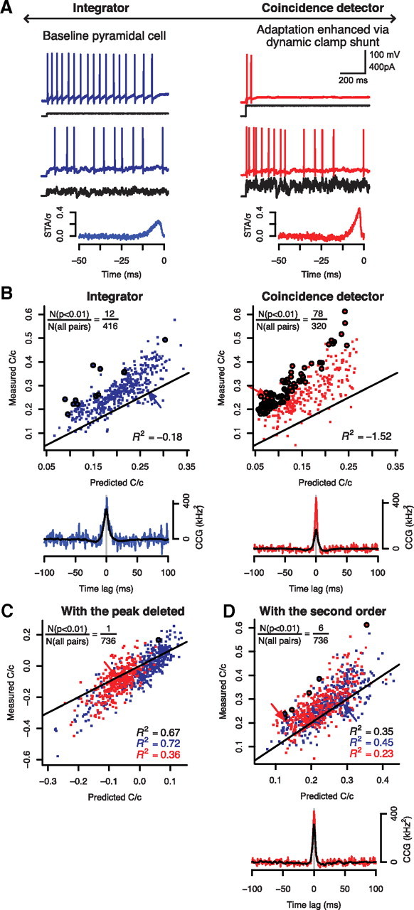
CA1 pyramidal neurons operating preferentially in a coincidence detector-mode exhibit greater spike-time synchronization than when operating in an integrator-mode. A, Responses from a typical regular spiking pyramidal neuron to constant and fluctuating (τ = 5 ms) input are shown without any manipulation (left) and with a virtual shunt (10 nS, −70 mV reversal potential) inserted by dynamic clamp (right). We used the shunt to enhance adaptation by depolarizing threshold, thereby shifting the neuron from acting preferentially as an integrator to acting preferentially as a coincidence detector, as shown previously (Prescott et al., 2006). Trials with and without dynamic clamp were interleaved to assess each neuron in both operating modes. The bottom panels show representative STA from each mode from one of the neurons comprising the pair used to sample CCGs (as indicated by arrows) in B–D. B, Following the same approach used for conductance-based models (Fig. 5), we plotted measured and predicted C/c for each “preferred” operating mode. The prediction here is based on Equation 29. The circles identify those points that deviated significantly from prediction (p < 0.01, t test). In the integrator-mode, only 12 of 416 points showed significant deviation of the measured C/c from prediction, while significantly more points (78 of 320) showed significant deviation in the coincidence detector-mode (p < 0.001, χ² test); in other words, the first-order prediction was less consistent for the coincidence detector-mode. The arrows point to data for which sample CCGs are shown. Predicted CCGs (black) deviated from measured CCGs (color) the same way as in Figure 5A. Data are from a total of 12 cells. C, Measured and predicted C/c values for both operating modes were replotted after removing data ±2 ms around the peak in the CCGs. As in Figure 5C, excluding excess synchrony not predicted on the basis of rate comodulation gave a closer match between measured and predicted C/c values, leaving only one data point (circled) that deviated significantly from prediction (p < 0.01, t test). D, Likewise, inclusion of second-order terms (i.e., Eq. 31) in our prediction gave a dramatically improved match, leaving only three data points (circled) for each operating mode with significant deviation from prediction (p < 0.01, t test). The improved prediction of spike-time synchrony afforded by inclusion of the second-order correction is also evident from the sample CCG (compare Fig. 5D).

Slice preparation and electrophysiology

Experimental protocols were approved by the University of Pittsburgh Institutional Animal Care and Use Committee and have been previously described (Prescott et al., 2006). Briefly, adult male Sprague Dawley rats were anesthetized with intraperitoneal injection of sodium pentobarbital (50–75 mg/kg) and perfused intracardially with ice-cold oxygenated (95% O₂ and 5% CO₂) sucrose-substituted artificial CSF (ACSF) containing the following (in mm): 252 sucrose, 2.5 KCl, 2 CaCl₂, 2 MgCl₂, 10 glucose, 26 NaHCO₃, 1.25 NaH₂PO₄, and 5 kynurenic acid. The brain was rapidly removed and sectioned coronally to give 300-μm-thick slices, which were kept in normal oxygenated ACSF (126 mm NaCl instead of sucrose and without kynurenic acid) at room temperature until recording.

Slices were transferred to a recording chamber constantly perfused with oxygenated (95% O₂ and 5% CO₂) ACSF heated to 31 ± 1°C. Pyramidal neurons in the CA1 region of hippocampus were recorded in the whole-cell configuration with >70% series resistance compensation using an Axopatch 200B amplifier (Molecular Devices). Membrane potential (after correction for the liquid junction potential of 9 mV) was adjusted to −70 mV through tonic current injection. Intracellular recording solution contained the following (in mm): 125 KMeSO₄, 5 KCl, 10 HEPES, and 2 MgCl₂, 4 ATP (Sigma-Aldrich), 0.4 GTP (Sigma-Aldrich), as well as 0.1% Lucifer yellow; pH was adjusted to 7.2 with KOH. Pyramidal morphology was confirmed with epifluorescence after recording. All experiments were performed in 10 μm bicuculline methiodide (Sigma-Aldrich), 10 μm CNQX (6-cyano-7-nitroquinoxaline-2,3-dione) (Sigma-Aldrich), and 40 μm d-AP-5 (d-2-amino-5-phosphonovaleric acid) (Ascent Scientific) to block background synaptic activity.

Stimuli (see above) were injected into the recorded neurons through the patch pipette. To manipulate spike threshold mechanism (see Results), an artificial “shunt” conductance (E_shunt = −70 mV, g_shunt = 10 nS) was applied via dynamic clamp implemented with a Digidata 1200A ADC/DAC board (Molecular Devices) and DYNCLAMP2 software (Pinto et al., 2001) running on a dedicated processor as previously described (Prescott et al., 2006; Prescott and De Koninck, 2009); update rate was 10 kHz. Traces were low-pass filtered at 2 kHz and digitized at 10 kHz using a CED 1401 computer interface (Cambridge Electronic Design).

Reverse correlation analysis

For simulation and experimental data, we calculated spike-triggered averages (STAs) and covariance of stimuli (STC). The STA is simply the average of the set of stimuli that led to spikes subtracted from the mean of the prior stimulus distribution (i.e., the distribution of all stimuli independent of spiking output). Here, to remove the ambiguities caused by the temporal correlations, we used the fluctuating part of the unfiltered stimulus, $I\left(t\right)=\sigma \left(\sqrt{c}{\xi }_{\text{c}}\left(t\right)+\sqrt{1-c{\xi }_{\text{i}}}\left(t\right)\right)$; in other words, we used ξ(t) instead of ζ(t) (see Eq. 2). Therefore, we have the following:

The time window for the STA was 200 ms before each spike, which captured most of the STA power. In a similar way, the STC and spike-triggered correlation of stimuli (STCor) Q(t,t′) are given by Bialek and de Ruyter Van Steveninck (1988) as follows:

where Cov_spike and Cov_prior are the covariance matrices of the spike-triggered and prior stimuli, respectively. The STA and STCor were used for predicting a cross-correlogram (CCG) in the first- and second-order by Equations 29 and 31, respectively (see below, Predicting CCGs from reverse correlation analysis). Predicted spike train covariance and correlation were computed from the CCG in the same way as the measured CCGs (see below).

Calculation of the measured CCG and correlation

We computed the CCGs of each spike train as follows. We started by building a spike train from the spike times with a Δt = 1 ms time bin and computed the CCGs via the time-averaged unbiased empirical correlation function (Perkel et al., 1967): when a spike train for neuron i and kth repetition is y_i,k(t), the cross-correlogram is given by the following:

where N_repeat is the number of repetitions, and L is the length of the spike trains and y_i,Nrepeat+1 = y_i,1.

From Equation 10, we computed the correlation of the spike-counts with the time window of size T as follows:

ϴ_T is a window function giving ϴ_T(t) = 1 if 0 ≤ t ≤ T and ϴ_T(t) = 0 otherwise. The shift correlator computes the covariance as follows:

and the correlation coefficient is given by ρ_T = C_T/(C₁C₂)^1/2 where the auto-covariance of each neuron C_i (i = 1,2) was calculated in the same way. Equations 10 and 12 are related as follows:

where Φ_T(t) is a triangular window function such that Φ_T(t) = |T − t| if −T ≤ t ≤ T and Φ_T(t) = 0 otherwise (Bair et al., 2001). Therefore, C_T as well as ρ_T were computed from CCGs via Equation 13.

In our analysis, we always computed the full CCGs and tried to analyze their behavior both at long and short timescales. The time window size T was not as important as in de la Rocha et al. (2007); therefore, in every case, we used T = 200 ms and dropped T from the notations.

Statistical analysis

We calculated the variance of the covariance, Var[C], by computing the bootstrap statistics of <y₁(0)y₂(τ)τ_shuffle in Equation 10; at each step, we constructed a resampled cross-correlogram <y₁(0)y₂(τ)τ_resample by random resampling from <y₁(0)y₂(τ)τ_shuffle and computed <n₁n₂τ_resample by Equation 12. We collected 400 <n₁n₂τ_resample with which the variance became stable. The Var[C] is taken as this resample variance and C is also recalibrated with the resample mean as follows:

For experimental data in Figure 7B–D, t scores were calculated from C and Var[C]. However, as for the simulation data, we could arbitrarily add more repetitions to suppress Var[C] down to sufficiently low level. For the analytic prediction, Var[C] could be computed in a similar way, but it was always insignificant (<1% of the covariance) for both experimental and simulation data.

In Figures 5 and 7, we evaluated the predictive power of the predicted C in terms of the coefficient of determination, R², defined by the following:

By definition, R² = 1 signifies the perfect match, while the prediction has no correlation with the measured C when R² = 0. In some cases, R² < 0, and this signifies that the predictions in fact diverge away from the data with a different average.

Predicting CCGs from reverse correlation analysis

Here, we derive the first- and second-order prediction presented as Equations 29–32 in Results by using the reverse correlation analysis of the linear–nonlinear (LN) cascade model (Victor and Shapley, 1980; Meister and Berry, 1999). The LN model is composed of two stages: first, the stimulus I(t) was linear filtered by the relevant features of the model {ε_α} (α = 1, 2, …, D), and the probability to spike at the given time bin [t, t + Δt], P(spike|x) where

Here, as above (see Reverse correlation analysis), we use the unfiltered stimulus $I\left(t\right)=\sigma \left(\sqrt{c}{\xi }_{\text{c}}\left(t\right)+\sqrt{1-c{\xi }_{\text{i}}}\left(t\right)\right)$. Since the actual injected stimulus and I(t) are linearly related, STA and STCor have the same temporal correlation as the actual stimulus, and, consequently, the temporal correlation naturally shows up in the predicted CCGs; for example, compare predicted CCGs for τ = 5 and 50 ms in Figure 5B.

We follow the same derivation as in the study by de la Rocha et al. (2007): the common noise part δI = $\sqrt{c}\sigma {\xi }_{\text{c}}$ will be regarded as the perturbation on top of I₀ = I(t)|_c=0 and the comodulated part of the firing rate will be determined by Wiener series expansion in δI.

First-order prediction (see Results, Eqs. 29, 30).

The firing rate change induced by a small perturbation I₀ → I₀ + δI can be approximated as follows:

where δI(t) has Gaussian statistics with a variance σ² (Rieke et al., 1999; Hong et al., 2008). STA represents the spike-triggered average of stimuli. Then the correlation function of q(t) = P(spike at t) is as follows:

where <δI₁(0)δI₂(τ)τ = cσ₁σ₂δ(τ) if δI_i = $\sqrt{c}\delta {\xi }_{\text{c}}$. This is essentially the same derivation of the correlation–gain relationship based on the linear response theory (de la Rocha et al., 2007; Hong et al., 2008) since the STA is the linear kernel relating the stimulus and firing rate as in Equation 17.

We now define the firing rate v(t) = q(t)/Δt and the predicted cross-correlogram for each pair as follows:

which is Equation 29 in Results. Furthermore, if we use the identity (Chialvo et al., 1997; Hong et al., 2008),

the firing rate covariance is given by the following:

where we changed the variables in the third line as t″ = t + t′. The last line is equivalent to the original relationship between the correlation and gain (see Results, Eq. 30) (de la Rocha et al., 2007; Shea-Brown et al., 2008).

Second-order prediction (see Results, Eqs. 31, 32).

When we include the second-order term in Equation 17, we obtain the following (Rieke et al., 1999; Hong et al., 2008):

where Q(t₁,t₂) is the STCor in Equation 9. The contribution to the CCG, Equation 31 in Results, is obtained in a straightforward way, as follows:

Note that we excluded the self-contraction to generate a proper Wiener series (Rieke et al., 1999).

In particular, when we have the same input condition, μ₁ = μ₂ = μ and σ₁ = σ₂ = σ, for the same type of neuron as in Figures 3 and 6, the peak height at t = 0 is given by the following:

Figure 3.

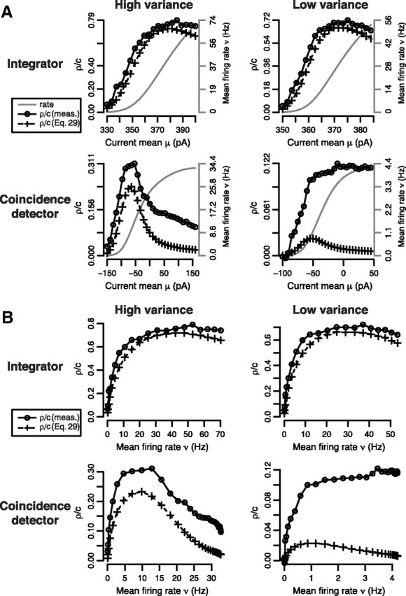
Output correlation is sensitive to stimulus variance in coincidence detectors, unlike in integrators, and has a variable relationship with output rate. A, Using the same conductance-based models as in Figure 2, the integrator (top) and coincidence detector (bottom) were stimulated with high- and low-variance input: σ_high² = 400 pA² and σ_low² = 100 pA² for the integrator; σ_high² = 2000 pA² and σ_low² = 520 pA² for the coincidence detector. Output rate ν and correlation ρ measured from simulations (○) together with ρ predicted from Equation 29 (+) were plotted against input mean μ. In B, ρ was replotted against ν to visualize the correlation–rate relationship. The range of ν (gray) varies between panels because of differences in maximal firing rate across cell types and stimulus conditions (Fig. 2A). For the integrator, ρ increased with ν and was quite accurately predicted by Equation 29 in both the high- and low-variance conditions. For the coincidence detector, ρ decreased for ν > 10 Hz in the high-variance condition, which was only qualitatively predicted from Equation 29, and the prediction was even less accurate in the low-variance condition. These results demonstrate that output correlation in coincidence detectors is higher than predicted on the basis of rate comodulation, and is accentuated under stimulus conditions in which ∂ν/∂μ is low. Given that rate comodulation should be minimized under those conditions (Fig. 1D), correlation in excess of the prediction might be attributable to some mechanism other than rate comodulation. In every case, input correlation was c = 0.3.

Figure 6.

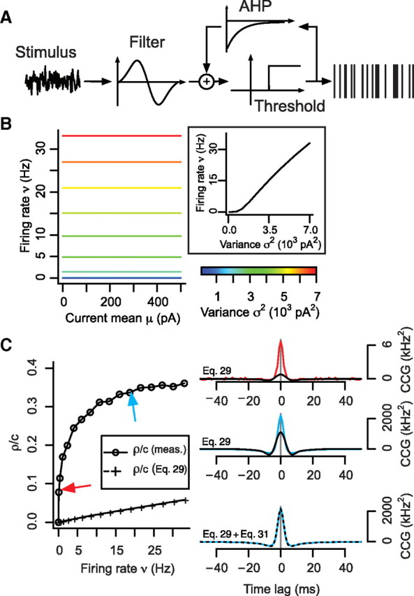
Phenomenological model sensitive only to stimulus variance exhibits correlated spiking due uniquely to spike-time synchronization. A, FT model was constructed by coupling a biphasic filter (reminiscent of the coincidence detector STA; Fig. 2C) and a step-function representing threshold. B, Because of its filter properties, the FT model is uniquely sensitive to stimulus fluctuations. Firing rate gain with respect to μ is zero but is positive with respect to σ. C, Using the stimulation paradigm shown in Figure 1A, a pair of FT models were given correlated input with equal μ and σ; c = 0.5; τ = 5 ms. Measured ρ/c values increased with ν, despite the first-order prediction (Eq. 29) giving a much smaller correlation, which vanishes as the time window size T increases (data not shown) on the basis of ∂ν/∂μ equaling 0. The arrows point to data for which sample CCGs are shown. Predicted CCGs (black) deviated from measured CCGs (color) in the same manner as when the first-order prediction (Eq. 29) was applied to the conductance-based coincidence detector model in Figure 5A. When second-order terms were included (Eq. 31), the predicted CCG was much more accurate (bottom).

Furthermore, we consider the case when the neuron is effectively well described by a single preferred spike-evoking stimulus feature (PSESF), ε(t), such as when the neuron functions almost as a pure integrator or a pure coincidence detector. In this case, Q(t₁,t₂) can be written as Q(t₁,t₂) = Y(t₁)Y(t₂), where Y(t) ∝ ε(t), and therefore

From ${\displaystyle \int Q\left(t_1,t_1\right)d{t}_1}$ = σ³(∂v/∂σ)/v (Hong et al., 2008), the predicted peak height becomes

which is equivalent to Equation 32 in Results. Therefore, the firing rate gain with respect to stimulus variance contributes to the CCG peak height.

Note in the case of a single PSESF that the input mean and variance sensitivity of the firing rate are related as follows (Hong et al., 2008):

where

Therefore, when ε̄ ≠ 0, as in the pure integrator, the contribution of the peak to the correlation is suppressed compared with the first-order prediction, Equation 30. In the pure coincidence detector, on the other hand, ε̄ = 0, but firing rate ν is also independent of μ (see Fig. 6B), which can still make ∂ν/∂σ finite. Therefore, the predicted correlation in the pure coincidence detector [based on Eqs. 29, 30, and ν(μ) = constant] (Barreiro et al., 2010) will be profoundly modified by the quadratic-order approximation (see Results, Simulations in a phenomenological coincidence detector model).

Results

When two or more neurons receive correlated (i.e., shared) input, their output spike trains should exhibit some correlation despite the effects of independent input (Fig. 1A). Spike train covariance C and the correlation coefficient ρ (i.e., C normalized by spike train variance) should, therefore, carry information about the input correlation c. However, de la Rocha et al. (2007) showed that the relationship between input and output correlation (denoted correlation susceptibility S = ρ/c) depends on the mean μ and variance σ² of the input (Fig. 1B). This is important because stimulus-dependent changes in S prevent one-to-one mapping between input correlation and output correlation. Correlation-based coding is straightforward if S is independent of μ and σ² (Fig. 1C, left), but it is compromised or requires a more complicated decoding scheme if S varies with μ and σ² (Fig. 1C, right).

One way of understanding why this occurs is that, for a given input correlation, output correlation will vary depending on the sensitivity (i.e., gain) of the firing rate ν of each neuron with respect to the stimulus mean μ: if stimulus fluctuations occur within a steep region of the ν–μ curve, rate will fluctuate widely in each cell and the pair will exhibit large comodulated rate fluctuations, whereas stimulus fluctuations within a shallow region of the ν–μ curve will logically drive smaller comodulated rate fluctuations (Fig. 1D). Consequently, ρ “inherits” the same tuning as ν(μ), even when c is fixed; under these conditions, c cannot be unambiguously decoded from ρ without knowledge of μ. This line of reasoning triggered three concerns: (1) it applies to rate comodulation but not necessarily to spike-time synchronization, and thus it neglects one component of output correlation; (2) it implicitly assumes that input fluctuations are “noise” rather than “signal”; and (3) output rate and synchronization (i.e., correlation based on spike-time synchronization as opposed to rate comodulation) are liable to be tuned to different stimulus properties. This led us to our overall hypothesis that some cell types may encode signal-dependent fluctuations with precise spike-time synchronization and can do so independently of rate-based coding of other stimulus features.

The dependence of output rate ν on input parameters μ and σ differs fundamentally between cell types, as shown in Figure 2 for our conductance-based models: ν is principally sensitive to μ in the case of integrators, whereas it is also very sensitive to σ in the case of coincidence detectors (Higgs et al., 2006; Arsiero et al., 2007; Lundstrom et al., 2008). For simulations reported here, input was treated as a continuous stream rather than as discrete synaptic inputs (Destexhe et al., 2001); nonetheless, σ reflects coordinated fluctuations in presynaptic activity (Fellous et al., 2003), the temporal structure of which is reflected in the autocorrelation time τ (shorter τ implies more precise synchrony), while c specifies the proportion of inputs shared between two postsynaptic neurons. The first two parameters, σ and τ, affect the temporal precision of spiking in each postsynaptic neuron, while c affects correlation across neurons—all three parameters ultimately affect output synchrony.

Figure 2.

Integrators and coincidence detectors are sensitive to different stimulus statistics. Data here are based on simulations in conductance-based models (see Materials and Methods). A, In the integrator (left), ν was sensitive to μ but was relatively insensitive to σ, whereas ν was sensitive to both μ and σ in the coincidence detector (right). The insets highlight the differential ability of each cell type to encode σ; black and gray curves correspond to arrows on ν–μ plots. Notably, firing rate variation with σ may reflect the rate of brief, suprathreshold input events rather than the (rate-encoded) magnitude of those events. B, Sample traces show differential responsiveness of each cell type to constant and fluctuating input. The coincidence detector responds preferentially to fast stimulus transients because its voltage-dependent currents implement a high-pass filter. The integrator also responds to fast stimulus fluctuations, but its voltage-dependent currents encourage repetitive spiking even when input is constant. C, The differential requirements for spike generation are evident from the spike-triggered-averaged response (STA) to fluctuating input. D, The CCG corresponds to the overlap integral of the STA from each neuron within a pair. Therefore, pairs of integrators are predicted to exhibit broad, monophasic CCGs (left), whereas pairs of coincidence detectors are predicted to exhibit narrow, biphasic CCGs based on the typical shape of their STA (right).

The greater sensitivity of coincidence detectors to input synchrony relative to integrators (Fig. 2A,B) is a direct consequence of active membrane properties: activation of outward current (or inactivation of inward current) at perithreshold potentials helps ensure spike generation selectively in response to fast stimulus fluctuations (i.e., synchronous inputs), whereas perithreshold-activating inward current (or inactivating outward current) encourages repetitive spiking in response to constant or slow-changing input (Fourcaud-Trocmé et al., 2003; Svirskis et al., 2004; Higgs et al., 2006; Arsiero et al., 2007; Lundstrom et al., 2008; Prescott et al., 2008a). Differential sensitivity to input synchrony can be demonstrated most succinctly by contrasting which stimulus features preferentially elicit spikes in each cell type. We estimated the preferred spike-eliciting stimulus feature as the spike-triggered-averaged stimulus (STA) of the response of each cell to noisy input (see examples in Fig. 2B). The integrator exhibits a relatively broad, monophasic STA (Fig. 2C, left), whereas the coincidence detector exhibits a biphasic STA with a positive phase that is remarkably narrow (Fig. 2C, right).

The shape of the STA should, in theory, relate directly to the cross-correlation of output spiking given that the CCG is the overlap integral of the STA of each neuron, according to the first-order approximation in c (see Materials and Methods) (de la Rocha et al., 2007), as follows:

Hence, the broad monophasic integrator STA predicts a broad monophasic CCG for pairs of integrators (Fig. 2D, left), whereas the narrow biphasic coincidence detector STA predicts a narrow biphasic CCG for pairs of coincidence detectors (Fig. 2D, right). Using the relationship between the STA and firing rate, the covariance C of the output spike count is as follows (see Materials and Methods):

which is consistent with the study by de la Rocha et al. (2007) because sensitivity (or gain) of ν with respect to μ is the dominant factor determining the degree of correlated spiking given a certain degree of input correlation (Fig. 1D). Strong dependence of the relationship between ρ and c (i.e., correlation susceptibility S) on μ is not conducive to correlation-based coding (Fig. 1C, right). However, the STA does not always accurately represent the preferred spike-eliciting stimulus feature (this occurs when spike generation is sensitive to higher-order stimulus statistics), which invalidates predictions based on Equation 29 in certain cases (see below).

We therefore set out to identify (1) whether and how correlation susceptibility S(μ,σ) differs between integrators and coincidence detectors, (2) what the consequences of such differences are for correlation-based coding, and (3) precisely why the stimulus dependence of S differs between cell types.

Simulations in conductance-based integrator and coincidence detector models

To compare the correlation susceptibility S (=ρ/c) of integrators and coincidence detectors, we conducted a series of numerical simulations using pairs of model neurons receiving a mix of correlated and independent input (Fig. 1A). For each neuron type, we varied mean μ under high- or low-variance σ² conditions, and evaluated the output rate ν and correlation ρ (Fig. 3). As illustrated in Figure 2A, maximal ν differs between cell types and between σ conditions, which leads to unavoidable differences in the range of ν on each panel of Figure 3. Nevertheless, the ν(μ) curves (gray) are similarly shaped in all four conditions. If ρ simply inherited the same tuning as ν with respect to μ, then ρ(μ) curves should also be similarly shaped—clearly, they are not.

As expected for integrators, ρ/c increased to a maximum <1 as μ was increased in both the high and low σ cases (Fig. 3A, top). In coincidence detectors, however, a similar pattern was observed in the low σ case, but not in the high σ case, in which ρ/c decreased after reaching a peak (Fig. 3A, bottom). Figure 3B shows the same data replotted with ν on the x-axis. For coincidence detectors receiving high σ input, the correlation–rate relationship was strongly negative at high rates. The same coincidence detectors receiving low σ input exhibited little change in correlation across most of the (albeit narrow) range of firing rates, which implies that S is not significantly dependent on μ or ν in this cell type under these conditions. This property should be conducive to good correlation-based coding (see below).

To investigate how the stimulus dependence of S affects correlation-based coding by integrators and coincidence detectors, we measured ρ in response to different combinations of c and μ (Fig. 4A). As predicted, S was strongly dependent on μ in the case of integrators, which caused encoding of c by ρ to be ambiguous; in contrast, S was relatively unaffected by μ in the case of coincidence detectors, consistent with good correlation-based coding (compare Fig. 1C). Notably, Equation 29 failed to accurately predict ρ in the case of coincidence detectors (Fig. 4A, inset) despite having worked in the case of integrators (see below).

Figure 4.

Correlation-based coding by integrators and coincidence detectors. A, We measured output correlation ρ in response to different combinations of mean μ and input correlation c (top). Curves on 2-D plots correspond to horizontal cross-sections, at different μ, through 3-D plots (bottom; compare Fig. 1C). Tight clustering of ρ–c curves despite differences in μ is conducive to good correlation-based coding by coincidence detectors (right), which contrasts to the broad distribution of those curves for integrators (left). Equivalent plots for the coincidence detector based on prediction by Equation 29 (inset) shows that the first-order prediction clearly fails to account for output correlation among coincidence detectors. Noticeably, ρ is smaller among coincidence detectors than among integrators. This stems from differences in the CCG, typical examples of which are shown in B based on measurement from pairs of each cell type with the same mean firing rate of 12 Hz; c = 0.3. These measured CCGs confirmed CCG shapes predicted in Figure 2D. Small values of ρ do not necessarily compromise synchrony transfer and correlation-based coding, whereas stimulus-dependent variability in S does (see text). In parts A and B, σ² = 100 pA² for the integrator and σ² = 1000 pA² for the coincidence detector.

Small values of ρ observed among coincidence detectors stem from the shape of coincidence detector CCGs, which are narrow and biphasic, unlike integrator CCGs, which are broad and monophasic (Fig. 4B; compare prediction in Fig. 2D). Small values of ρ do not imply that synchrony transfer will fail, because downstream coincidence detectors prefer tall, narrow CCGs among their upstream neurons rather than short, broad CCGs, regardless of the absolute magnitude of ρ (S. Hong, S. A. Prescott, and E. De Schutter, unpublished observations). To summarize, correlation-based coding is viable despite small ρ as long as the relationship between ρ and c is insensitive to other stimulus features like μ. These data demonstrate the feasibility of correlation-based coding among coincidence detectors.

Next, we asked why S(μ,σ) differs between integrators and coincidence detectors. In all panels of Figure 3, ρ/c values predicted from Equation 29 were plotted for comparison with measured ρ/c values. The derivation of Equation 29 is based on linear response theory and requires several assumptions that are not strictly met in our simulations such as very small c. However, despite comparable stimulus parameters and identical methods used to calculate output correlation, Equation 29 predicted most of the output correlation observed for integrators but only a fraction of that observed for coincidence detectors. In the latter case, the degree of inaccuracy appeared to depend on σ. We reasoned that identifying why Equation 29 fails to accurately predict output correlation in coincidence detectors, especially under certain stimulus conditions, would help identify how correlated spiking in coincidence detectors differs from that in integrators.

To test the accuracy of the prediction, we plotted predicted covariance against measured covariance in Figure 5. If prediction by Equation 29 were consistently accurate (i.e., for all stimulus conditions), all data points would lie along the diagonal line. Figure 5A illustrates the consistent accuracy of the prediction for pairs of integrators versus its inconsistency for pairs of coincidence detectors. These data represent responses to a broad range of different μ and σ. The important observation is that the first-order prediction was reasonably accurate for all stimulus conditions in the case of integrators, whereas it was grossly inaccurate for many stimulus conditions in the case of coincidence detectors. Whereas Figure 3 illustrates stimulus conditions for which prediction by Equation 29 is good or bad, Figure 5 focuses on why Equation 29 sometimes fails to predict output correlation among coincidence detectors. By plotting covariance C rather than the correlation coefficient ρ, Figure 5A confirms that the prediction error seen for coincidence detectors is not attributable to autovariances in the spike train. Sample CCGs (Fig. 5A, right) reveal that the predicted CCG differs most from the measured CCG at the central peak; this is true for both integrators and coincidence detectors, but it translates into a larger discrepancy in predicting overall output correlation as the CCG gets narrower. Thus, these data qualitatively confirmed our starting predictions and identified a quantitative shortfall in the ability of Equation 29 to predict output correlation, especially in coincidence detectors.

In addition to reflecting the stimulus features to which each cell type is most sensitive, we reasoned that the width of the CCG also reflects the autocorrelation time of the correlated signal (which can be taken to reflect the temporal precision of spiking in presynaptic neurons) (see above). Therefore, we lengthened τ from 5 to 50 ms for simulations in Figure 5B based on the hypothesis that widening the CCG might reduce the prediction error. As expected, lengthening τ improved the prediction for both integrators and coincidence detectors but, whereas the CCG for the integrators was dramatically widened, the CCG for coincidence detectors remained narrow and the prediction still exhibited a sizeable error near the peak of the CCG. To determine whether prediction error near the peak of the CCG was sufficient to explain the discrepancy observed on the measured versus predicted C plots, we removed data within ±2 ms of the peaks of all coincidence detector CCGs and replotted the data for τ = 5 ms—this amounts to preferentially removing precisely synchronized spikes from the calculation of total output correlation. The result was a near-perfect prediction by Equation 29 (Fig. 5C), meaning the prediction error near the peak of narrow CCGs was sufficient to explain the failure of the prediction in coincidence detectors for all input conditions for which the original prediction was poor.

Next, we investigated (1) whether and how the original prediction might be improved so that the predicted CCG would more accurately match the measured CCG for coincidence detectors at the central peak, and (2) whether this would improve the measured versus predicted C plots (as expected given the results in Fig. 5C). We reasoned that if coincidence detectors are sensitive to stimulus variance (Fig. 2), then the prediction (Eq. 29) should take into account how stimulus variance affects spike generation. Therefore, we incorporated a second-order term into the prediction based on the following:

where Q(t,t′) is the spike-triggered correlation of the stimuli (STCor) (see Materials and Methods for derivation). Total output correlation should thus be predicted by the combination of Equations 29 and 31. For conditions in which input statistics and preferred spike-eliciting stimulus feature are equal, Equation 31 predicts the additional peak height as follows:

Using Equation 31, we find that the coincidence detector CCG was much better predicted at its central peak (Fig. 5D, right) and measured C was accurately predicted for a broad range of input conditions (Fig. 5D, left). Successfully modifying our quantitative prediction by incorporating Equation 31 argues that the difference in threshold mechanism is critical insofar as spike generation in integrators is preferentially sensitive to first-order stimulus statistics, whereas spike generation in coincidence detectors is also sensitive to second-order stimulus statistics (Fig. 2). On a more practical note, our ability to modify our quantitative prediction so that it works consistently (i.e., for all stimulus conditions) for integrators as well as for coincidence detectors confirms that we did not violate any fundamental assumption to the point of invalidating the prediction as a whole.

In principle, the second-order contribution (Eq. 31) can decrease much more quickly than the first-order prediction (Eq. 29) as the input correlation c becomes smaller. However, we found that the first-order prediction remained inconsistent for coincidence detectors even at relatively small values of c (Fig. 5E, left) and that including second-order terms significantly improved that prediction (Fig. 5E, right). In fact, measured C was closely matched by the second-order prediction across a broad range of c, and both were much larger than the first-order prediction except for very small c (Fig. 5F), proving that our result is not an artifact of large input correlations.

The nonlinear contribution to precise spike-time synchrony is not necessarily limited to second-order terms, and indeed the remaining systematic deviations from our second-order prediction in Figure 5, D and E, suggest that even higher-order terms contribute to synchrony, although that contribution is evidently quite small. Quantifying the nth order nonlinearity becomes more difficult for higher n, as the dimensionality of the nth moment of the spike-triggering stimuli rapidly increases, and was considered beyond the scope of the present study.

Simulations in a phenomenological coincidence detector model

For the conductance-based models described above, the difference in threshold mechanism between integrators and coincidence detectors derives from distinct spike initiation dynamics (Prescott et al., 2008a). Based on results from phenomenological models without “dynamics” (de la Rocha et al., 2007), one might suspect that the specific dynamics of the cell model are not vital for the correlation–rate relationship. The type of threshold and the dynamical mechanism responsible for “thresholding” are inextricably linked, but, nonetheless, to test whether the type of threshold is critical rather than the dynamics per se, we constructed a phenomenological coincidence detector model comprising a filter and threshold in which the filter is biphasic, like the STA in our conductance-based coincidence detector model (Fig. 6A; compare Fig. 2C). In this dynamics-free model, ν was completely independent of μ but varied with σ (Fig. 6B; compare Fig. 2A, right)—in effect, this model constitutes an “ideal” coincidence detector. Despite the first-order prediction (i.e., Eq. 29) that there should be no output correlation (given that ∂ν/∂μ = 0) (Barreiro et al., 2010), pairs of ideal coincidence detectors receiving correlated input did indeed exhibit correlated spiking (Fig. 6C, left). Moreover, sample CCGs (Fig. 6C, right) were comparable in shape to those of the conductance-based coincidence detector model (compare Figs. 4, 5). Furthermore, the same prediction error was observed near the peak of the narrow CCGs when applying Equation 29, but our quantitative prediction was near-perfect when second-order terms (Eq. 31) were included. Overall, these results argue that the type of threshold used by a pair of neurons receiving correlated input will impact the correlation in their output.

To summarize results up to this point, ideal coincidence detectors (exemplified by our FT model) exhibit correlations arising solely from spike-time synchronization. In contrast, more realistic coincidence detectors (exemplified by our conductance-based HHLS model) exhibit a mixture of spike-time synchronization and rate comodulation, whereas realistic integrators (exemplified by our conductance-based ML model) exhibit mostly rate comodulation. The timescales of these two types of output correlation differ but nonetheless overlap. More importantly, the two types of output correlation exhibit fundamentally different sensitivities to firing rate: rate comodulation varies with firing rate, whereas spike-time synchronization does not. We predicted that real neurons should exhibit rate comodulation and spike-time synchronization if those neurons operate at least partially as coincidence detectors and, moreover, that the predominance of each type of output correlation will depend on the balance of operating modes.

Experiments in CA1 pyramidal neurons made to behave preferentially as integrators or coincidence detectors via manipulation of threshold mechanism by dynamic clamp

Integrators and coincidence detectors are found throughout the nervous system but tend to exhibit specializations beyond threshold mechanism. Because those additional specializations could confound our comparison of correlation susceptibility, we chose to compare correlation susceptibility in a single type of neuron whose threshold mechanism was experimentally manipulated such that the neuron behaves preferentially as an integrator or coincidence detector.

Pyramidal neurons, including those in the CA1 region of hippocampus, display the hallmarks of integrators when recorded in acute brain slices but behave more like coincidence detectors upon introduction of a virtual leak conductance by dynamic clamp (Fig. 7A), consistent with a predicted switch in threshold mechanism (Prescott et al., 2006, 2008b). Thus, by manipulating the membrane properties of CA1 pyramidal neurons, we were able to compare correlation susceptibility in a single cell type operating preferentially in one or the other mode—the shift in operating mode is quantitative, not absolute. In the interests of comparing experimental and simulation data [and to compare with past studies (de la Rocha et al. (2007)], we applied the same stimulation paradigm used in simulations (i.e., noisy current injection) together with the simplest dynamic-clamp manipulation capable of switching the threshold mechanism (i.e., constant leak conductance).

Compared with STAs in the integrator-mode (Fig. 7A, left), STAs in the coincidence detector-mode (Fig. 7A, right) had a higher peak height, and were therefore steeper than integrator STAs, but the negative phase was far less prominent than in STAs from our coincidence detectors models (compare Fig. 2C). This is likely due to spike initiation in real neurons being influenced by more currents with gating variables spanning a broader range of timescales than were included in our minimal conductance-based models. In any case, as we would predict, the steep weakly biphasic STAs are consistent with the narrow weakly biphasic CCGs observed for pyramidal neurons in the coincidence detector-mode (see below). Most importantly for our purposes, firing rate gain with respect to μ, which is proportional to how biphasic the STA is (Eq. 20), was significantly lower in the coincidence detector-mode compared with the default integrator-mode (0.14 ± 0.041 vs 0.05 ± 0.016 Hz/pA; p < 0.01, t test), whereas firing rate gain with respect to σ was similar between modes (0.034 ± 0.022 vs 0.022 ± 0.011 Hz/pA), which means ∂ν/∂σ was, relative to ∂ν/∂μ, higher in the coincidence detector-mode (0.25 ± 0.16 vs 0.50 ± 0.29; p < 0.01, t test). This is consistent with the differential response properties reported for the conductance-based models in Figure 2A. Like for simulation data in Figure 5, we plotted our experimental data as measured versus predicted C based on the first-order prediction described in Equation 29 (Fig. 7B, top). As expected, the prediction error was much greater for the coincidence detector-mode than for the integrator-mode, which was also evident in the sample CCGs (Fig. 7B, bottom). Consistent with simulations (compare Figs. 4, 5, CCGs), the CCG for the coincidence detector-mode was much narrower than for the integrator-mode, and the first-order prediction deviated from the measured CCG primarily at its peak (Fig. 7B, bottom). As for simulation data, we hypothesized that removing a narrow region around the peak of the CCG (where the actual and predicted CCGs differ most) would dramatically improve the prediction as visualized on the measured versus predicted C plots, which indeed it did (Fig. 7C). Similarly, including the second-order terms described by Equation 31 improved our prediction, especially for the coincidence detector-mode (Fig. 7D). These experiments demonstrate that pyramidal neurons receiving shared input can exhibit output correlation in excess of that predicted from firing rate comodulation, and that this spike-time synchronization is greater when the neurons behave more like coincidence detectors.

Discussion

Through simulations and experiments, we have shown that pairs of neurons receiving correlated input can exhibit spiking that is correlated in different ways, and that the overall contribution of each type of output correlation depends on intrinsic cellular properties. Ideal integrators exhibit output correlations comprised entirely of rate comodulation. This makes sense given that individual integrators use rate encoding in which spiking is dictated by the mean (i.e., a first-order statistic) of the input; therefore, input can be reconstructed entirely by applying a first-order filter (i.e., the STA) to the spike train. Conversely, ideal coincidence detectors exhibit output correlations comprised entirely of spike-time synchronization (Fig. 6). However, realistic coincidence detectors exhibit output correlations comprised partly of spike-time synchronization and partly of rate comodulation (Fig. 5). This too makes sense given that individual coincidence detectors use temporal encoding in which spiking is sensitive to the variance (i.e., a second-order statistic) of the input; therefore, reconstructing the input from the spike train requires inclusion of first- and second-order filters (Theunissen and Miller, 1995). Real neurons and realistic conductance-based models are never pure integrators or coincidence detectors. We have juxtaposed the two operating modes for didactic purposes, but, ultimately, operating mode is a continuum representing the interplay between stimulus kinetics and neural dynamics. Neural dynamics—most notably spike generation—differ between neurons, can be modulated within a given neuron, and directly impact how a neuronal ensemble encodes and transmits information.

Some cell types are optimized for integration or coincidence detection; for example, many neurons early in the auditory pathway (e.g., cochlear nucleus and superior olive) are exquisite coincidence detectors (Manis and Marx, 1991; Cao et al., 2007; Mathews et al., 2010), whereas certain neurons in the entorhinal cortex are near-perfect integrators (Egorov et al., 2002). In addition to morphological specializations (Agmon-Snir et al., 1998), a broad range of ion currents can influence operating mode, the common feature being that such currents activate or inactivate at voltages near threshold, or that they impact the gating of other perithreshold currents, for example, by shifting voltage threshold (Prescott et al., 2006, 2008a). Whether pyramidal neurons in the neocortex and hippocampus function as integrators or coincidence detectors has been controversial (Abeles, 1982; Softky and Koch, 1993; Shadlen and Newsome, 1998). The answer depends not only on intrinsic cell properties but also on stimulus conditions (Rudolph and Destexhe, 2003) and other external factors like background synaptic activity that influence membrane conductance (Destexhe et al., 2003). Shunting and adaptation, especially in combination, can encourage coincidence detection in pyramidal neurons that might otherwise behave preferentially as integrators (Prescott et al., 2006, 2008b). The adaptation current I_M has been shown to encourage coincidence detection in hippocampal and neocortical pyramidal neurons (Hu et al., 2007; Guan et al., 2011) and is itself subject to endogenous modulators and to several drugs (for review, see Brown and Passmore, 2009). This supports the view that pyramidal neurons (and presumably other cell types through adaptation by I_M and via other mechanisms) can shift between operating modes. By not operating at one or the other extreme, pyramidal neurons can flexibly use rate- and/or synchrony-based coding (see below).

The coexistence of rate- and synchrony-based coding is consistent with recent modeling work showing that differently encoded information can be simultaneously propagated through feedforward networks depending on network properties (Kremkow et al., 2010; Kumar et al., 2010). Our results emphasize the importance of cellular properties for exactly the same issues. Network and cellular properties can be intimately related (see above regarding synaptic input and membrane conductance) and may interact nonlinearly such that forms of modulation, which individually have weak effects, combine to produce powerful gating mechanisms that switch a network between propagating synchronous or asynchronous activity (see below). But it is not necessarily the case that synchronous and asynchronous spikes act independently; for example, in spiny stellate cells receiving thalamocortical input via a limited number of weak synapses, asynchronous background cortical input may be crucial for setting the membrane potential of stellate cells close enough to spike threshold that synchronous thalamic inputs can elicit spikes (Douglas and Martin, 2007; da Costa and Martin, 2011). In that example, asynchronous input may facilitate the propagation of synchronous spiking and, furthermore, might act as a continuously variable gain-control mechanism rather than as a simple on–off switch.

An important related issue is correlation between excitatory and inhibitory input. This has been proposed as a mechanism to regulate information transmission (Salinas and Sejnowski, 2001; Kremkow et al., 2010), amplify external inputs (Murphy and Miller, 2009), and enhance response fidelity (Wehr and Zador, 2003; Cafaro and Rieke, 2010). Such correlations may exist with delays of only a few milliseconds, likely because of feedforward inhibition ensuring a narrow integration window (Wehr and Zador, 2003; Higley and Contreras, 2006). Under those conditions, presynaptic spikes synchronized with millisecond precision are required to reliably evoke responses in postsynaptic neurons.

Information encoded by rate or synchrony must be reliably transmitted (when allowed by gating mechanisms) and eventually decoded. Unambiguous decoding requires independent rate- and correlation-based coding (Fig. 1). Recent findings (de la Rocha et al., 2007) have cast doubt on this independence. We concur that a correlation–rate relationship compromises correlation-based coding based on rate comodulation, but we demonstrate here that output correlation and rate can be correlated without interfering with synchrony-based coding. Counting spikes neglects the information carried by spike timing. The absolute timing of spikes in a single presynaptic cell has little impact on postsynaptic activation, but the relative timing of spikes across multiple presynaptic cells is crucial if the postsynaptic cell operates as a coincidence detector; by extension, the absolute timing of synchronized volleys likely carries information about the original stimulus.

It follows that integrators exhibit the correlation–rate relationship described by de la Rocha et al. (2007), but that same relationship, although it can be observed in coincidence detectors (Barreiro et al., 2010), applies to only a fraction (i.e., to only one component) of their output correlation. Notably, de la Rocha et al. used computer models in which spike generation depended on mean input (i.e., integration) and the 1-s-long stimuli used in their experiments were sufficiently short that slow adaptation was minimal, thus favoring spike generation based on mean input (Prescott and Sejnowski, 2008). In addition to testing “integrator” models, we tested conductance-based and phenomenological models in which spike generation depends on input variance (i.e., coincidence detector models). Our experiments were conducted with 300-s-long stimuli to favor adaptation, our rationale being that neurons in vivo exist in a chronically depolarized and shunted state because of synaptic bombardment (Destexhe et al., 2003). By testing a single cell type under different “virtual network conditions” rather than testing different cell types representing each extreme of the continuum between integration and coincidence detection, our results show that the neuronal operating mode can be shifted along that continuum and that this shift in operating mode adjusts the balance of rate- and synchrony-based coding.

These results demonstrate the importance of cell-level properties for network-level coding. There has been a longstanding bias in the network modeling community to focus on synaptic weights and network architecture, with far less emphasis put on cellular properties. Here, we have shown what happens when neurons do not “integrate and fire.” Similarly, Burak et al. (2009) and Barreiro et al. (2010) recently showed differences in output correlation depending on the type of model used. Effects of synaptic kinetics, background noise, and input spike train statistics on output correlation have also been documented (Maex et al., 2000; Tetzlaff et al., 2008; Ostojic et al., 2009). Tchumatchenko et al. (2010) have shown specifically that output correlations can be rate dependent or independent according to input conditions. Our results emphasize how both types of correlations can coexist and that this depends on input conditions and (how that input is encoded given) single cell firing properties. Indeed, whereas simplified models tend to favor pure integration or pure coincidence detection, real neurons and realistic conductance-based models exhibit a context-dependent mixture of operating modes. Neglecting the richness of cell-level coding properties will surely translate into underestimation of network-level coding possibilities.

In conclusion, different types of neurons or even the same neuron operating under different conditions can be differentially sensitive to first- and second-order stimulus statistics, namely mean and variance. If we do not assume that fluctuations are simply noise, and if a neuron is sensitive to those fluctuations (which is true of coincidence detectors), then output spiking should carry information about the signal variance. Two such neurons receiving correlated input may carry information about signal variance in their precisely synchronized spiking. Even if correlated with firing rate (indeed, such output correlations might arise from correlations between features of the original input), spike-time synchronization is separate from rate comodulation, which, by definition, is directly linked to the firing rate that is tuned to the signal mean. Both forms of correlation may coexist and operate independently. Thus, the richness of single-neuron coding abilities translates into even richer multineuron coding possibilities.

References

- Abeles M. Role of the cortical neuron: integrator or coincidence detector? Isr J Med Sci. 1982;18:83–92. [PubMed] [Google Scholar]
- Abeles M. Corticonics: neural circuits of the cerebral cortex. Cambridge, MA: Cambridge UP; 1991. [Google Scholar]
- Aertsen A, Diesmann M, Gewaltig MO. Propagation of synchronous spiking activity in feedforward neural networks. J Physiol Paris. 1996;90:243–247. doi: 10.1016/s0928-4257(97)81432-5. [DOI] [PubMed] [Google Scholar]
- Agmon-Snir H, Carr CE, Rinzel J. The role of dendrites in auditory coincidence detection. Nature. 1998;393:268–272. doi: 10.1038/30505. [DOI] [PubMed] [Google Scholar]
- Arsiero M, Lüscher HR, Lundstrom BN, Giugliano M. The impact of input fluctuations on the frequency–current relationships of layer 5 pyramidal neurons in the rat medial prefrontal cortex. J Neurosci. 2007;27:3274–3284. doi: 10.1523/JNEUROSCI.4937-06.2007. [DOI] [PMC free article] [PubMed] [Google Scholar]
- Averbeck BB, Latham PE, Pouget A. Neural correlations, population coding and computation. Nat Rev Neurosci. 2006;7:358–366. doi: 10.1038/nrn1888. [DOI] [PubMed] [Google Scholar]
- Bair W, Zohary E, Newsome WT. Correlated firing in macaque visual area MT: time scales and relationship to behavior. J Neurosci. 2001;21:1676–1697. doi: 10.1523/JNEUROSCI.21-05-01676.2001. [DOI] [PMC free article] [PubMed] [Google Scholar]
- Barreiro AK, Shea-Brown E, Thilo EL. Time scales of spike-train correlation for neural oscillators with common drive. Phys Rev E Stat Nonlin Soft Matter Phys. 2010;81 doi: 10.1103/PhysRevE.81.011916. 011916. [DOI] [PubMed] [Google Scholar]
- Bialek W, de Ruyter Van Steveninck RR. Real-time performance of a movement-sensitive neuron in the blowfly visual system: coding and information transfer in short spike sequences. Proc R Soc Lond B Biol Sci. 1988;234:379–414. [Google Scholar]
- Brown DA, Passmore GM. Neural KCNQ (Kv7) channels. Br J Pharmacol. 2009;156:1185–1195. doi: 10.1111/j.1476-5381.2009.00111.x. [DOI] [PMC free article] [PubMed] [Google Scholar]
- Burak Y, Lewallen S, Sompolinsky H. Stimulus-dependent correlations in threshold-crossing spiking neurons. Neural Comput. 2009;21:2269–2308. doi: 10.1162/neco.2009.07-08-830. [DOI] [PubMed] [Google Scholar]
- Cafaro J, Rieke F. Noise correlations improve response fidelity and stimulus encoding. Nature. 2010;468:964–967. doi: 10.1038/nature09570. [DOI] [PMC free article] [PubMed] [Google Scholar]
- Cao XJ, Shatadal S, Oertel D. Voltage-sensitive conductances of bushy cells of the mammalian ventral cochlear nucleus. J Neurophysiol. 2007;97:3961–3975. doi: 10.1152/jn.00052.2007. [DOI] [PubMed] [Google Scholar]
- Chialvo DR, Longtin A, Müller-Gerking J. Stochastic resonance in models of neuronal ensembles. Phys Rev E Stat Nonlin Soft Matter Phys. 1997;55:1798–1808. [Google Scholar]
- da Costa NM, Martin KA. How thalamus connects to spiny stellate cells in the cat's visual cortex. J Neurosci. 2011;31:2925–2937. doi: 10.1523/JNEUROSCI.5961-10.2011. [DOI] [PMC free article] [PubMed] [Google Scholar]
- de la Rocha J, Doiron B, Shea-Brown E, Josić K, Reyes A. Correlation between neural spike trains increases with firing rate. Nature. 2007;448:802–806. doi: 10.1038/nature06028. [DOI] [PubMed] [Google Scholar]
- Destexhe A, Rudolph M, Fellous JM, Sejnowski TJ. Fluctuating synaptic conductances recreate in vivo-like activity in neocortical neurons. Neuroscience. 2001;107:13–24. doi: 10.1016/s0306-4522(01)00344-x. [DOI] [PMC free article] [PubMed] [Google Scholar]
- Destexhe A, Rudolph M, Paré D. The high-conductance state of neocortical neurons in vivo. Nat Rev Neurosci. 2003;4:739–751. doi: 10.1038/nrn1198. [DOI] [PubMed] [Google Scholar]
- Douglas RJ, Martin KA. Mapping the matrix: the ways of neocortex. Neuron. 2007;56:226–238. doi: 10.1016/j.neuron.2007.10.017. [DOI] [PubMed] [Google Scholar]
- Egorov AV, Hamam BN, Fransén E, Hasselmo ME, Alonso AA. Graded persistent activity in entorhinal cortex neurons. Nature. 2002;420:173–178. doi: 10.1038/nature01171. [DOI] [PubMed] [Google Scholar]
- Engel AK, Roelfsema PR, Fries P, Brecht M, Singer W. Role of the temporal domain for response selection and perceptual binding. Cereb Cortex. 1997;7:571–582. doi: 10.1093/cercor/7.6.571. [DOI] [PubMed] [Google Scholar]
- Fellous JM, Rudolph M, Destexhe A, Sejnowski TJ. Synaptic background noise controls the input/output characteristics of single cells in an in vitro model of in vivo activity. Neuroscience. 2003;122:811–829. doi: 10.1016/j.neuroscience.2003.08.027. [DOI] [PMC free article] [PubMed] [Google Scholar]
- Fourcaud-Trocmé N, Hansel D, van Vreeswijk C, Brunel N. How spike generation mechanisms determine the neuronal response to fluctuating inputs. J Neurosci. 2003;23:11628–11640. doi: 10.1523/JNEUROSCI.23-37-11628.2003. [DOI] [PMC free article] [PubMed] [Google Scholar]
- Gerstner W, Kreiter AK, Markram H, Herz AV. Neural codes: firing rates and beyond. Proc Natl Acad Sci U S A. 1997;94:12740–12741. doi: 10.1073/pnas.94.24.12740. [DOI] [PMC free article] [PubMed] [Google Scholar]
- Guan D, Higgs MH, Horton LR, Spain WJ, Foehring RC. Contributions of Kv7-mediated potassium current to sub- and suprathreshold responses of rat layer II/III neocortical pyramidal neurons. J Neurophysiol. 2011;106:1722–1733. doi: 10.1152/jn.00211.2011. [DOI] [PMC free article] [PubMed] [Google Scholar]
- Higgs MH, Slee SJ, Spain WJ. Diversity of gain modulation by noise in neocortical neurons: regulation by the slow afterhyperpolarization conductance. J Neurosci. 2006;26:8787–8799. doi: 10.1523/JNEUROSCI.1792-06.2006. [DOI] [PMC free article] [PubMed] [Google Scholar]
- Higley MJ, Contreras D. Balanced excitation and inhibition determine spike timing during frequency adaptation. J Neurosci. 2006;26:448–457. doi: 10.1523/JNEUROSCI.3506-05.2006. [DOI] [PMC free article] [PubMed] [Google Scholar]
- Hines ML, Carnevale NT. The NEURON simulation environment. Neural Comput. 1997;9:1179–1209. doi: 10.1162/neco.1997.9.6.1179. [DOI] [PubMed] [Google Scholar]
- Hong S, Lundstrom BN, Fairhall AL. Intrinsic gain modulation and adaptive neural coding. PLoS Comput Biol. 2008;4:e1000119. doi: 10.1371/journal.pcbi.1000119. [DOI] [PMC free article] [PubMed] [Google Scholar]
- Hu H, Vervaeke K, Storm JF. M-channels (Kv7/KCNQ channels) that regulate synaptic integration, excitability, and spike pattern of CA1 pyramidal cells are located in the perisomatic region. J Neurosci. 2007;27:1853–1867. doi: 10.1523/JNEUROSCI.4463-06.2007. [DOI] [PMC free article] [PubMed] [Google Scholar]
- König P, Engel AK, Singer W. Integrator or coincidence detector? The role of the cortical neuron revisited. Trends Neurosci. 1996;19:130–137. doi: 10.1016/s0166-2236(96)80019-1. [DOI] [PubMed] [Google Scholar]
- Kremkow J, Aertsen A, Kumar A. Gating of signal propagation in spiking neural networks by balanced and correlated excitation and inhibition. J Neurosci. 2010;30:15760–15768. doi: 10.1523/JNEUROSCI.3874-10.2010. [DOI] [PMC free article] [PubMed] [Google Scholar]
- Kumar A, Rotter S, Aertsen A. Spiking activity propagation in neuronal networks: reconciling different perspectives on neural coding. Nat Rev Neurosci. 2010;11:615–627. doi: 10.1038/nrn2886. [DOI] [PubMed] [Google Scholar]
- Lundstrom BN, Hong S, Higgs MH, Fairhall AL. Two computational regimes of a single-compartment neuron separated by a planar boundary in conductance space. Neural Comput. 2008;20:1239–1260. doi: 10.1162/neco.2007.05-07-536. [DOI] [PMC free article] [PubMed] [Google Scholar]
- Maex R, Vos BP, De Schutter E. Weak common parallel fibre synapses explain the loose synchrony observed between rat cerebellar Golgi cells. J Physiol. 2000;523:175–192. doi: 10.1111/j.1469-7793.2000.t01-1-00175.x. [DOI] [PMC free article] [PubMed] [Google Scholar]
- Mainen ZF, Sejnowski TJ. Reliability of spike timing in neocortical neurons. Science. 1995;268:1503–1506. doi: 10.1126/science.7770778. [DOI] [PubMed] [Google Scholar]
- Manis PB, Marx SO. Outward currents in isolated ventral cochlear nucleus neurons. J Neurosci. 1991;11:2865–2880. doi: 10.1523/JNEUROSCI.11-09-02865.1991. [DOI] [PMC free article] [PubMed] [Google Scholar]
- Mathews PJ, Jercog PE, Rinzel J, Scott LL, Golding NL. Control of submillisecond synaptic timing in binaural coincidence detectors by Kv1 channels. Nat Neurosci. 2010;13:601–609. doi: 10.1038/nn.2530. [DOI] [PMC free article] [PubMed] [Google Scholar]
- Meister M, Berry MJ. The neural code of the retina. Neuron. 1999;22:435–450. doi: 10.1016/s0896-6273(00)80700-x. [DOI] [PubMed] [Google Scholar]
- Murphy BK, Miller KD. Balanced amplification: a new mechanism of selective amplification of neural activity patterns. Neuron. 2009;61:635–648. doi: 10.1016/j.neuron.2009.02.005. [DOI] [PMC free article] [PubMed] [Google Scholar]
- Ostojic S, Brunel N, Hakim V. How connectivity, background activity, and synaptic properties shape the cross-correlation between spike trains. J Neurosci. 2009;29:10234–10253. doi: 10.1523/JNEUROSCI.1275-09.2009. [DOI] [PMC free article] [PubMed] [Google Scholar]
- Palanca BJ, DeAngelis GC. Does neuronal synchrony underlie visual feature grouping? Neuron. 2005;46:333–346. doi: 10.1016/j.neuron.2005.03.002. [DOI] [PubMed] [Google Scholar]
- Perkel DH, Gerstein GL, Moore GP. Neuronal spike trains and stochastic point processes. II. Simultaneous spike trains. Biophys J. 1967;7:419–440. doi: 10.1016/S0006-3495(67)86597-4. [DOI] [PMC free article] [PubMed] [Google Scholar]
- Pinto RD, Elson RC, Szücs A, Rabinovich MI, Selverston AI, Abarbanel HD. Extended dynamic clamp: controlling up to four neurons using a single desktop computer and interface. J Neurosci Methods. 2001;108:39–48. doi: 10.1016/s0165-0270(01)00368-5. [DOI] [PubMed] [Google Scholar]
- Prescott SA, De Koninck Y. Impact of background synaptic activity on neuronal response properties revealed by stepwise replication of in vivo-like conditions in vitro. In: Destexhe A, Bal T, editors. The dynamic clamp: from principles to applications. New York: Springer; 2009. pp. 89–114. [Google Scholar]
- Prescott SA, Sejnowski TJ. Spike-rate coding and spike-time coding are affected oppositely by different adaptation mechanisms. J Neurosci. 2008;28:13649–13661. doi: 10.1523/JNEUROSCI.1792-08.2008. [DOI] [PMC free article] [PubMed] [Google Scholar]
- Prescott SA, Ratté S, De Koninck Y, Sejnowski TJ. Nonlinear interaction between shunting and adaptation controls a switch between integration and coincidence detection in pyramidal neurons. J Neurosci. 2006;26:9084–9097. doi: 10.1523/JNEUROSCI.1388-06.2006. [DOI] [PMC free article] [PubMed] [Google Scholar]
- Prescott SA, De Koninck Y, Sejnowski TJ. Biophysical basis for three distinct dynamical mechanisms of action potential initiation. PLoS Comput Biol. 2008a;4:e1000198. doi: 10.1371/journal.pcbi.1000198. [DOI] [PMC free article] [PubMed] [Google Scholar]
- Prescott SA, Ratté S, De Koninck Y, Sejnowski TJ. Pyramidal neurons switch from integrators in vitro to resonators under in vivo-like conditions. J Neurophysiol. 2008b;100:3030–3042. doi: 10.1152/jn.90634.2008. [DOI] [PMC free article] [PubMed] [Google Scholar]
- Reyes AD. Synchrony-dependent propagation of firing rate in iteratively constructed networks in vitro. Nat Neurosci. 2003;6:593–599. doi: 10.1038/nn1056. [DOI] [PubMed] [Google Scholar]
- Rieke F, Warland D, Bialek W. Spikes: exploring the neural code. Cambridge, MA: MIT; 1999. [Google Scholar]
- Rudolph M, Destexhe A. Tuning neocortical pyramidal neurons between integrators and coincidence detectors. J Comput Neurosci. 2003;14:239–251. doi: 10.1023/a:1023245625896. [DOI] [PubMed] [Google Scholar]
- Salinas E, Sejnowski TJ. Correlated neuronal activity and the flow of neural information. Nat Rev Neurosci. 2001;2:539–550. doi: 10.1038/35086012. [DOI] [PMC free article] [PubMed] [Google Scholar]
- Schneidman E, Berry MJ, 2nd, Segev R, Bialek W. Weak pairwise correlations imply strongly correlated network states in a neural population. Nature. 2006;440:1007–1012. doi: 10.1038/nature04701. [DOI] [PMC free article] [PubMed] [Google Scholar]
- Schreiber S, Fellous JM, Tiesinga P, Sejnowski TJ. Influence of ionic conductances on spike timing reliability of cortical neurons for suprathreshold rhythmic inputs. J Neurophysiol. 2004;91:194–205. doi: 10.1152/jn.00556.2003. [DOI] [PMC free article] [PubMed] [Google Scholar]
- Shadlen MN, Movshon JA. Synchrony unbound: a critical evaluation of the temporal binding hypothesis. Neuron. 1999;24:67–77. 111–125. doi: 10.1016/s0896-6273(00)80822-3. [DOI] [PubMed] [Google Scholar]
- Shadlen MN, Newsome WT. The variable discharge of cortical neurons: implications for connectivity, computation, and information coding. J Neurosci. 1998;18:3870–3896. doi: 10.1523/JNEUROSCI.18-10-03870.1998. [DOI] [PMC free article] [PubMed] [Google Scholar]
- Shea-Brown E, Josić K, de la Rocha J, Doiron B. Correlation and synchrony transfer in integrate-and-fire neurons: basic properties and consequences for coding. Phys Rev Lett. 2008;100:108102. doi: 10.1103/PhysRevLett.100.108102. [DOI] [PubMed] [Google Scholar]
- Singer W. Synchronization of cortical activity and its putative role in information processing and learning. Annu Rev Physiol. 1993;55:349–374. doi: 10.1146/annurev.ph.55.030193.002025. [DOI] [PubMed] [Google Scholar]
- Softky WR, Koch C. The highly irregular firing of cortical cells is inconsistent with temporal integration of random EPSPs. J Neurosci. 1993;13:334–350. doi: 10.1523/JNEUROSCI.13-01-00334.1993. [DOI] [PMC free article] [PubMed] [Google Scholar]
- Svirskis G, Kotak V, Sanes DH, Rinzel J. Sodium along with low-threshold potassium currents enhance coincidence detection of subthreshold noisy signals in MSO neurons. J Neurophysiol. 2004;91:2465–2473. doi: 10.1152/jn.00717.2003. [DOI] [PMC free article] [PubMed] [Google Scholar]
- Tchumatchenko T, Malyshev A, Geisel T, Volgushev M, Wolf F. Correlations and synchrony in threshold neuron models. Phys Rev Lett. 2010;104 doi: 10.1103/PhysRevLett.104.058102. 058102. [DOI] [PubMed] [Google Scholar]
- Tetzlaff T, Rotter S, Stark E, Abeles M, Aertsen A, Diesmann M. Dependence of neuronal correlations on filter characteristics and marginal spike train statistics. Neural Comput. 2008;20:2133–2184. doi: 10.1162/neco.2008.05-07-525. [DOI] [PubMed] [Google Scholar]
- Theunissen F, Miller JP. Temporal encoding in nervous systems: a rigorous definition. J Comput Neurosci. 1995;2:149–162. doi: 10.1007/BF00961885. [DOI] [PubMed] [Google Scholar]
- Tiesinga P, Fellous JM, Sejnowski TJ. Regulation of spike timing in visual cortical circuits. Nat Rev Neurosci. 2008;9:97–107. doi: 10.1038/nrn2315. [DOI] [PMC free article] [PubMed] [Google Scholar]
- Treisman A. Solutions to the binding problem: progress through controversy and convergence. Neuron. 1999;24:105–110. 111–125. doi: 10.1016/s0896-6273(00)80826-0. [DOI] [PubMed] [Google Scholar]
- Uhlenbeck GE, Ornstein LS. On the theory of Brownian motion. Phys Rev. 1930;36:823–841. [Google Scholar]
- Victor J, Shapley R. A method of nonlinear analysis in the frequency domain. Biophys J. 1980;29:459–483. doi: 10.1016/S0006-3495(80)85146-0. [DOI] [PMC free article] [PubMed] [Google Scholar]
- Wehr M, Zador AM. Balanced inhibition underlies tuning and sharpens spike timing in auditory cortex. Nature. 2003;426:442–446. doi: 10.1038/nature02116. [DOI] [PubMed] [Google Scholar]
- Wolfe J, Houweling AR, Brecht M. Sparse and powerful cortical spikes. Curr Opin Neurobiol. 2010;20:306–312. doi: 10.1016/j.conb.2010.03.006. [DOI] [PubMed] [Google Scholar]
- Zohary E, Shadlen MN, Newsome WT. Correlated neuronal discharge rate and its implications for psychophysical performance. Nature. 1994;370:140–143. doi: 10.1038/370140a0. [DOI] [PubMed] [Google Scholar]