Evaluating the physiological significance of respiratory sinus arrhythmia: looking beyond ventilation–perfusion efficiency

Abstract

We conducted a theoretical study of the physiological significance of respiratory sinus arrhythmia (RSA), a phenomenon used as an index of cardiac vagal tone and wellbeing, whereby the heart rate (HR) increases during inspiration and decreases during expiration. We first tested the hypothesis that RSA improves gas exchange efficiency but found that although gas exchange efficiency improved with slow and deep breathing and with increased mean heart rate, this was unrelated to RSA. We then formulated and tested a new hypothesis: that RSA minimizes the work done by the heart while maintaining physiological levels of arterial carbon dioxide. We tested the new hypothesis using two methods. First, the HR for which the work is minimized was calculated using techniques from optimal control theory. This calculation was done on simplified models that we derived from a previously published model of gas exchange in mammals. We found that the calculated HR was remarkably similar to RSA and that this became more profound under slow and deep breathing. Second, the HR was prescribed and the work done by the heart was calculated by conducting a series of numerical experiments on the previously published gas exchange model. We found that cardiac work was minimized for RSA-like HR functions, most profoundly under slow and deep breathing. These findings provide novel insights into potential reasons for and benefits of RSA under physiological conditions.

Key points

• Respiratory sinus arrhythmia (RSA) is the variation of heart rate with breathing: heart rate increases during inspiration and decreases during expiration.

• RSA is seen in many species including humans where it is strongest in the young and fit. The loss of RSA has been linked with cardiac mortality; however, the function of RSA is presently unknown.

• One hypothesis proposed previously is that RSA allows for more efficient gas exchange between the lungs and the blood.

• Our theoretical study does not support this hypothesis. Instead, a new hypothesis is proposed and tested using computational tools – that RSA helps the heart do less work while maintaining healthy levels of blood gases.

• Of course, this new hypothesis needs to be further tested both experimentally and by using more sophisticated mathematical models, but if correct, it could explain why inducing RSA artificially in patients with cardiovascular disease improves their health.

Introduction

In fit, healthy subjects, the heart rate (HR) is coupled to the respiratory cycle: the HR increases during inspiration and decreases during expiration. This phenomenon, known as respiratory sinus arrhythmia (RSA), is used as an index of cardiac vagal tone and contributes to heart rate variability (Grossman & Taylor, 2007). The mechanism of RSA and the factors affecting it have been studied extensively (Anrep et al. 1936; Taha et al. 1995; Paton et al. 2005, 2006), yet the physiological significance of RSA remains controversial (Larsen et al. 2010). It has been suggested by Hayano et al. (1996) that the physiological function of RSA is to match ventilation and perfusion in the lungs and thus optimise oxygen uptake and carbon dioxide removal. This hypothesis was supported by their experimental results for dogs where they induced RSA, inverse RSA and no RSA by clustering the heart beats during inspiration, during expiration and by evenly spreading the heart beats across the respiratory cycle. They showed that, in the presence of RSA, the dead space-to-tidal volume ratio and intrapulmonary shunt fraction decreased and that the oxygen uptake was enhanced (although this last result may not be statistically significant given that under control O₂ consumption was 71.9 ± 5.7 ml min⁻¹ and under artificial RSA it was 74.7 ± 9.6 ml min⁻¹). Hayano & Yasuma (2003) hypothesized that RSA is an intrinsic resting function of the cardiopulmonary system and suggested that matching ventilation to perfusion via RSA decreases the energy expenditure of the cardiopulmonary system by reducing the number of heart beats during expiration (Yasuma & Hayano, 2004). However, these additional suggestions were not explored further or tested directly.

Giardino et al. (2003) measured the ventilatory equivalents of CO₂ (/) and O₂ (/) during paced breathing in 10 healthy human volunteers and concluded that gas exchange efficiency increased with RSA. In contrast, Sin et al. (2010), compared the ventilatory equivalents of CO₂ and O₂ in patients with fixed-rate cardiac pacemakers against healthy control subjects during fast and slow paced breathing. They showed similar trends between the two groups and concluded that the improvements in gas exchange efficiency are unrelated to RSA in humans.

Motivated by the controversy of RSA, and given the abundance of experimental animal and human data, we decided to conduct a theoretical study of the physiological significance of RSA using mathematical models. As far as we know, such a theoretical study has not been conducted previously. While mathematical models that can mimic RSA exist, they are either phenomenological (McGuinness et al. 2004; Shiogai et al. 2010) and cannot be used to study gas exchange efficiency, or large scale (Lu et al. 2001; Kotani et al. 2002; Ursino & Magosso, 2003; Batzel et al. 2007; Cheng et al. 2010) and have been used to study other phenomena such as periodic breathing, the Valsalva manoeuver, regulation of heart period variability or cardio-respiratory synchronization. Many existing mathematical models take respiratory and cardiac control mechanisms into account (e.g. large scale models) or have an embedded hypothesized mechanism for the appearance of RSA (e.g. phenomenological models). These models make it impossible to separate the question of what the physiological function of RSA is from how RSA is generated.

We used a previously published model of gas exchange in mammals (Ben-Tal, 2006) to calculate gas exchange efficiency during fast, normal and slow paced breathing, but found that while gas exchange efficiency improved with slow and deep breathing and with increased mean HR, this was unrelated to RSA. In an attempt to find physiological conditions under which gas exchange efficiency improved directly due to RSA, we simplified the Ben-Tal (2006) model. Serendipitously, the new simpler model provided novel insights into the physiological function of RSA. We found that RSA minimizes the work done by the heart while maintaining physiological levels of the partial pressure of CO₂. The optimization problem we formulated was solved using techniques from optimal control theory and gave an optimal HR function that was remarkably similar to RSA. Inspired by this, we next conducted a series of numerical experiments using the Ben-Tal (2006) model with prescribed HR functions and computed the work done by the heart as well as the volumes of O₂ and CO₂ taken up or removed by the blood. These studies were compared with previously published experiments on both humans and dogs.

Methods

The theoretical study in this paper was conducted in two parts. Each part of the study was performed using different mathematical techniques and different models. The variables and parameters encountered in the paper are given in Appendix A.

Part I

In this part of the study the HR function was calculated using techniques from optimal control theory (Lenhart & Workman, 2007). This was performed by converting an optimization problem that consists of a quantity to be minimized and several equations to be satisfied simultaneously (called constraints) into a larger set of differential equations with boundary conditions (these are conditions at the start and end of the respiratory cycle). These equations were solved numerically using the bvp4c subroutine in MATLAB (see http://www.mathworks.com/products/matlab/index.html).

The optimal procedure requires mathematical models in which the HR is a continuous function. We therefore simplified a model published previously by Ben-Tal (2006) (see Appendix B) in which the blood flow is pulsatile (and therefore HR is a discrete function) and constructed a simplified model in which the HR (and therefore blood flow) is continuous. We derived four models with various simplified assumptions. The simplest model was used to derive the optimization problem and illustrate the mathematical technique used for solving it. The other models were used to calculate the optimal HR function under more realistic conditions. The models and their underlying assumptions are presented in the Results section and in Appendix C. All our calculations in this part were performed using typical parameters for humans (see Appendix A).

Part II

In this part of the study a series of numerical experiments were conducted whereby the Ben-Tal (2006) gas exchange model was solved as a system of differential equations with initial values (these are conditions at the start of the numerical simulation) using the subroutine radau5 (see http://www.unige.ch/~hairer/software.html), and the work done by the heart was calculated for various prescribed input HR functions. The prescribed HR functions increased linearly during inspiration and decreased linearly during expiration. In the first set of experiments, for a given HR variability, the mean HR was changed until the simulated mean arterial tension of CO₂ or O₂ reached a desired value. This set of experiments was performed using human parameters (see Appendix A and Ben-Tal, 2006 for references). In the second set of experiments, for a given HR variability and a given mean HR, gas volumes were calculated. This set of experiments was performed using typical parameters for humans and dogs (see Appendix A for references).

Results

Part I

Reduced physiological models

The reduced models were derived by simplifying a model described by Ben-Tal (2006). The full model equations are given in Appendix B for convenience. Model 1a and Model 1b (described below) were obtained by assuming that the respiratory exchange ratio is one (that is, the flux of CO₂ from the blood into the lungs is the same as the flux of O₂ from the lungs into the blood). This assumption leads to a decoupling of the equations for O₂ and CO₂ (that is, the equations for O₂ can be solved without any knowledge of CO₂ tensions and vice versa). We also assumed that the alveolar pressure and the lung volume are constant, ignoring any variation in these variables, but kept the air flow as a function of time. In Model 2, we relaxed the assumption of a constant respiratory exchange ratio and coupled the equations for O₂ and CO₂. Then, in Model 3, we allowed the alveolar pressure and the lung volume to vary. The equations for Model 2 and Model 3 are given in Appendix C.

Model 1a

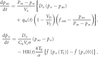
The equations for this model are as follows (see Appendix C for the derivation):

(1)

where p_ao is the alveolar partial pressure of O₂, is the averaged blood partial pressure of O₂ (over one heart period), P_m is the atmospheric pressure, p_w is water vapour pressure at body temperature, V_o is the mean alveolar volume, D_o is the oxygen diffusion capacity, q_in(t) is the inspired air flow, V_D is the dead-space volume, V_T is the tidal volume, f_om is the fractional dry concentration of O₂ in the atmosphere, C_u is a unit conversion factor, V_c is the capillary volume, HR(t) is the heart rate as a function of time, T_h is the haemoglobin concentration, σ is the solubility of O₂ in blood plasma, is the value of the haemoglobin saturation function at the end of the capillaries and is the value of the haemoglobin saturation function when the blood enter the lungs.

Model 1b

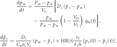
This model is similar to Model 1a but applies to CO₂ (see Appendix C for the derivation of these equations):

(2)

where p_ac is the alveolar partial pressure of CO₂ and is the averaged blood partial pressure of CO₂ (over one heart period). The recurring parameters in this model are the same as in Model 1a. The additional parameters are: D_c is the carbon dioxide diffusion capacity, is the solubility of CO₂ in blood plasma, r₂ is the dehydration reaction rate, is the hydration reaction rate and h is the concentration of H⁺ ions.

Model 2

This model is described by four differential equations (see Appendix C) with p_ao, , p_ac and as the variables. The respiratory exchange ratio could take any value (not just one as in Models 1a and 1b) and therefore O₂ and CO₂ are coupled. However, the alveolar pressure and the lung volume are still taken as constants as in Models 1a and 1b.

Model 3

This model is described by four differential equations for the same variables as in Model 2 (see Appendix C) except that now the alveolar pressure and the lung volume can oscillate.

Hydrodynamic analogy – gaining insight into the physiological relevance of RSA

Model 1a and Model 1b can be written more simply as follows (the equivalent symbols are given in Table 1):

Table 1.

Equivalent symbols in the simpler version of Model 1a and Model 1b

Symbol	O2 (Model 1a)	CO2 (Model 1b)
	pao	pac
u(t)	HR(t)	HR(t)
D1
D2
A
B
α1	fom	0
α2
β1	0.2113	pc(0)
β2	0	–1

(3)

The values for β₁ and β₂ in Model 1a were obtained by noting that near p_o= 104 mmHg, the saturation curve is almost flat and therefore the difference between the saturation values at the start and end of the capillaries, , can be approximated by a constant.

If α₂=β₂= 0, eqn (3) can be thought of as a hydrodynamic model (Fig. 1) where two water containers of fixed cross-sectional area are connected by a pipe at their base, with flow into the left-hand container and flow out of the right-hand container. The equations for the hydrodynamic model are given by:

Figure 1. The hydrodynamic model analogy of gas transport.

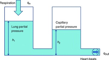
The left container represents the lungs and the right container represents the pulmonary capillaries.

(4)

where h₁ and h₂ are the heights of the water in the left and right containers, respectively, A₁ and A₂ are the cross-sectional areas of the left and right containers, respectively, D = D₁A₁=D₂A₂, and .

Consider the case when water is poured into the left container periodically, such that the flow into the left container is positive in the first half of the cycle and zero in the second half (this is analogous to inspired air flow). The flow out of the right container is controlled by a pump on the end of the outlet pipe. Assuming that the system must be in steady state, we asked the question of whether there is any advantage in operating the pump (or equivalently, changing the heart rate) in a particular way? By defining what this advantage is, we provide a possible answer to the question ‘what is the physiological significance of RSA?’. In the hydrodynamic model it is easy to see that in steady state, the volume of liquid that comes into the system over one cycle has to come out in the same time period (conservation of mass), and that therefore, the way the pump is controlled (or equivalently, the choice of HR) will not affect the volume of water that flows out of the right container – this is strictly determined by the input flow function . In other words, in this particular model of gas exchange, the amount of oxygen taken up by the blood (in steady state) cannot be affected by the heart rate, and therefore gas exchange efficiency cannot change due to the presence of RSA (or any other form of heart rate variability such as inverse RSA). However, as we show in the next section, one can choose a control function u(t) (representing the action of opening and closing the pump) such that a given amount of water (or equivalently, oxygen) is transported using less energy and that, interestingly, the optimal u(t) looks very much like RSA. This leads us to the formulation of a new hypothesis regarding the physiological significance of RSA, which we define mathematically in the next section.

Optimization problem

We assume that the heart pumps out a volume V_c at pressure P in a time interval T_L and that R_b is the resistance to flow, so that q=P/R_b is the blood flow. The volume of blood can then be calculated as follows:

from which we can find an expression for the pressure applied by the heart as a function of the volume: , where HR = 1/T_L is the heart rate. For an adiabatic process (that is, a process where there is no heat transfer), the work per heart beat is , the work per second is and the work per respiratory cycle with period T is given by

We assume that V_c and R_b are constants and therefore minimizing W_T is the same as minimizing E (defined below). While W_T is obviously a crude simplification, multiplying it by a constant will not change the results of the optimal control problem stated below. Moreover, we show later that the results do not change qualitatively in the more general case (representing a more complex relationship between the heart work and rate) where and n has values other than 2 (we checked values for 1.5 < n < 3).

We can now state the optimal control problem:

Find HR(t) such that is minimized subject to the following constraints:

1. The differential equations of the mathematical model are satisfied.

2. The system is in steady state.

3. The blood partial pressure of either O₂ or CO₂ has a given value on average over one breathing period.

The differential equations referred to in point 1 could be those of Model 1a, 1b, 2 or 3. To impose the steady state constraint in point 2 we require that the solution is periodic (i.e. the partial pressures at the start and at the end of the respiratory cycle are the same). The third constraint results in an additional equation where x represents oxygen or carbon dioxide, is the blood partial pressure and is the average of over one breathing period and has a given value. The problem formulated above can be solved for each of the four models (1a, 1b, 2 and 3) using standard techniques from optimal control theory described in Appendix D. The results are given in the next section.

Calculating the optimal HR function

In all the calculations that are shown here, q_in(t) is defined as (see also Fig. 2, top panel):

Figure 2. Typical calculations of optimal heart rate and partial pressures in Models 1a and 1b.

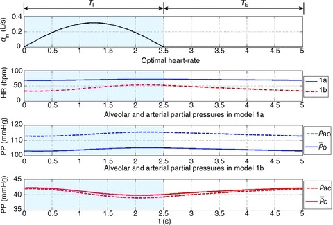
The inspired ventilation, q_in, is the same for both models (top panel). The shaded areas show the inspiration period. The averaged arterial partial pressure of O₂ () was constrained to 104 mmHg, the averaged arterial partial pressure of CO₂ () was constrained to 41 mmHg, and V_T= 0.5 l. All other parameters are the same as in Appendix A. Heart rate (HR) calculated for Model 1a – continuous line, HR calculated for Model 1b – dashed line. T_I and T_E are the inspiration and expiration periods, respectively. Note that O₂ and CO₂ are uncoupled.

where V_T is the tidal volume and T is the period of respiration. This choice gives . We chose the inspiration/expiration ratio (T_I/T_E) to be 1:1 as in Hayano et al. (1996) and Sin et al. (2010). The effect of other inspiration/expiration ratios is explored in Fig. 7 (see below for more details).

Figure 7. Increased T_I/T_E ratio leads to a weaker RSA and a growing phase-shift between the maximum heart rate and the end of inspiration.

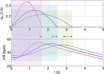
The calculation was performed using Model 1b. The shaded areas show the inspiration period for each case. The respiratory cycle is 5 s and V_T= 0.5 l in all cases. All other parameters are as in Appendix A. In blue T_I/T_E= 1:1, in red T_I/T_E= 1:2, and in black T_I/T_E= 2:1. The inspired ventilation, q_in, is shown in the top panel.

Typical outputs of the optimal calculation for Models 1a and 1b are shown in Fig. 2. The optimal HR is shown in the second panel. The continuous line shows the HR as calculated by using Model 1a and the dashed line shows the HR as calculated by using Model 1b. The third panel in Fig. 2 shows the blood and alveolar partial pressures of O₂ as calculated by Model 1a and the fourth panel shows the blood and alveolar partial pressures of CO₂ as calculated by Model 1b. It can be seen in Fig. 2 that the optimal HR function has an RSA-like shape (Taha et al. 1995) – it increases during inspiration and decreases during expiration – and also that the variation in HR is greater in Model 1b. The difference between p_ao and (the alveolar and arterial partial pressures of O₂) seen in the third panel is about 10 mmHg, which is not physiologically realistic (these two partial pressures are expected to have close values at the end of the capillaries). This difference persists in Models 2 and 3 but does not exist in the Ben-Tal (2006) model on which the reduced models are based. In the Ben-Tal (2006) model the blood partial pressures are initialized every heart beat. In the case of oxygen, the partial pressure falls to 40 mmHg (venous blood) every heart beat and takes a significantly longer time (compared with CO₂) to equilibrate again with the alveolar pressure before the next heart beat. The flux of oxygen from the lungs to the blood as a function of time in the Ben-Tal (2006) model thus deviates from the averaged, reduced models. A similar observation was made by Topor et al. (2004) who also reported a 10 mmHg difference in their averaged model. In many other averaged models this is not a problem because the assumption p_ao= is embedded in the model.

By plotting the inverse of the optimal HR we obtain the R-R interval (time-dependent heart beat period). Figure 3 shows such a plot for the optimal R-R interval calculated using Models 1b, 2 and 3 when the averaged was constrained. The shape of the R-R function as well as its magnitude look similar to reported measurements of RSA (see Discussion for more details). This feature as well as the reduction in the R-R interval during inspiration and increase in the R-R interval during expiration is preserved by all three models.

Figure 3. The RSA-like shape of the R-R interval is preserved by all three models.

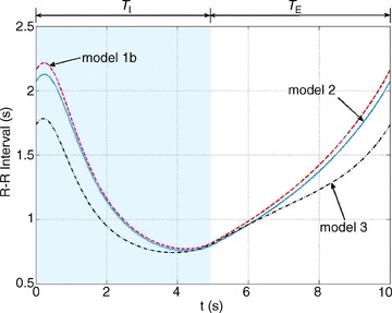
The calculation of the R-R interval for the different models was performed using the optimal control technique described in Appendix D and taking the inverse of the optimal heart rate. V_{T =} 1.0 l, T= 10 s, the averaged arterial partial pressure of CO₂ was constrained to 41.5 mmHg. T_I and T_E are the inspiration and expiration periods, respectively. The shaded area shows the inspiration period.

Figures 4–6 show how the optimal HR is affected by changing several physiological parameters: the averaged arterial partial pressure for CO₂ (Fig. 4, bottom three curves), the averaged arterial partial pressure for O₂ (Fig. 4, top three curves), the tidal volume (Fig. 5) and the respiratory period (Fig. 6). In Figs 5 and 6 we show only one example of the calculation performed using Model 1a to illustrate that the variation in the HR for Model 1b is greater. Figures 4–6 show that an increase in the desired levels of CO₂, in the tidal volume or in the respiratory period lead to an increase in the mean value and the variation of HR. This could be understood intuitively when thinking about the hydrodynamic analogy (and reversing the direction of flow): an increase in the amount of water that enters the left container will require an increase in the outflow (and therefore an increase in u(t), or HR) if the average levels of water in the right container need to stay the same.

Figure 4. Stronger RSA as a result of increased average arterial partial pressure of CO₂.

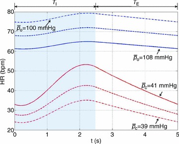
The optimal heart rate (HR) was calculated for Model 1a (top three curves) and Model 1b (bottom three curves) with V_T= 0.5 l. In Model 1b, the averaged arterial partial pressure of CO₂ was constrained to three values: 39 mmHg (dashed–dotted line), 40 mmHg (dashed line), 41 mmHg (continuous line). In Model 1a, the averaged arterial partial pressure of O₂ was constrained to: 100 mmHg (dashed–dotted line), 104 mmHg (dashed line), 108 mmHg (continuous line). T_I and T_E are the inspiration and expiration periods, respectively. The shaded area shows the inspiration period.

Figure 6. Stronger RSA with slow and deep breathing.

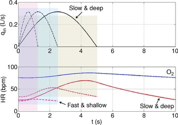
The optimal heart rate (HR) was calculated for Model 1a (labelled ‘O₂’) and Model 1b (remaining three curves). The shaded areas show the inspiration period for each breathing pattern. Only one cycle is shown. The inspired ventilation, q_in, is the same for both models (top panel). In Model 1b, the averaged arterial partial pressure of CO₂ was constrained to 41 mmHg. In Model 1a, the averaged arterial partial pressure of O₂ was constrained to 104 mmHg. Respiratory period and tidal volume were: T= 2.5 s, V_T= 0.25 l (dashed–dotted line); T= 5 s, V_T= 0.5 l (dashed line); T= 10 s, V_T= 1 l (continuous line). The minute ventilation was the same for all simulations: V_T/T= 0.1 l s⁻¹= 6 l min⁻¹. Only the case T= 10 s, V_T= 1 l is shown for Model 1a.

Figure 5. Stronger RSA with increased tidal volume when the arterial partial pressure of CO₂ is controlled (Model 1b).

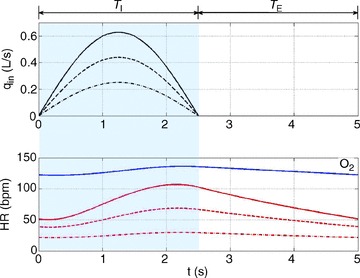
The optimal heart rate (HR) was calculated for Model 1a (labelled ‘O₂’) and Model 1b (remaining three curves). The inspired ventilation, q_in, is the same for both models (top panel). In Model 1b, the averaged arterial partial pressure of CO₂ was constrained to 40 mmHg. In Model 1a, the averaged arterial partial pressure of O₂ was constrained to 104 mmHg. Tidal volume took on the following three values: V_T= 0.4 l (dashed–dotted line), V_T= 0.7 l (dashed line), V_T= 1.0 l (continuous line). Only the case of V_T= 1.0 l is shown for Model 1a. T_I and T_E are the inspiration and expiration periods, respectively. The shaded area shows the inspiration period.

Figure 7 shows the effect of changing the inspiration/expiration ratio (while keeping minute ventilation the same) on RSA. A decrease in T_I/T_E (and an increase in tidal volume) leads to a stronger RSA. Interestingly, an increase in T_I/T_E also leads to a growing phase-shift between the time when maximum heart rate is reached and the end of inspiration.

Figure 13 shows that the calculation of the RSA-like heart rate is robust and is not affected qualitatively by changes to the expression of the work done by the heart.

Figure 13. The calculation of the RSA-like heart rate is not affected qualitatively by changes to the expression of the work done by the heart.

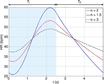
The calculations were performed by minimizing where n= 2 (dashed line), n= 1.5 (continuous line) or n= 3 (dashed–dotted line) and by using Model 1b.

Part II

Solving the model with a prescribed HR function

In this section we solve the Ben-Tal (2006) model (described in Appendix B) numerically when the HR function is prescribed. The HR in the Ben-Tal (2006) model is discrete but we can use a continuous function to calculate the times when the variables p_c, p_o and z need to be reinitialized (see Appendix B). The prescribed HR function increases linearly during the first half of the respiratory cycle and decreases linearly during the second half. Mathematically, this is expressed as follows:

where m is the mean HR and is the HR variability (the difference between the highest and lowest HR values – see Fig. 8 for the continuous HR and Fig. 9 for the analogous pulsatile HR). In the first set of numerical experiments, for a given value of Δ, we estimate the value of m for which the average arterial partial pressure of CO₂ or O₂ reaches a desired value (this is done by repeating the simulation for several values of m and interpolating). We then calculate E at that point as:

Figure 8. A saw-tooth HR function used to mimic RSA.

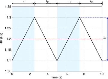
The parameter Δ governs the degree of RSA while m is the mean heart rate (HR). Here we took m= 1.2 Hz = 72 beats min⁻¹, Δ= 0.2 Hz = 12 beats min⁻¹. The shaded area shows the inspiration period.

Figure 9. Mimicking pulsatile blood flow (discrete heart rate).

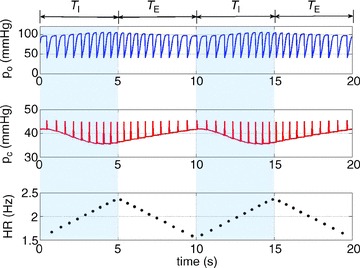
The arterial partial pressure of CO₂ (p_c, middle panel) and the arterial partial pressure of O₂ (p_o, top panel) are initialized for every heart beat. The heart rate shown here is taken at the minimum of the continuous curve in Fig. 10 with Δ= 0.84 Hz, mean HR = 1.9605 Hz. T_I and T_E are the inspiration and expiration periods, respectively. The shaded areas show the inspiration period.

(5)

Note that our calculation is true when the HR function is continuous. When the HR is discrete one can calculate the energy using numerical integration. Both calculations give the same results qualitatively (see Supplementary Fig. S4) but eqn (5) is easier to use and provides more insight.

In thyye second set of experiments, the model is solved numerically for given values of Δ and m and the volumes of O₂ and CO₂ taken up or removed by the blood are calculated:

and

Figures 10 and 11 show the normalized energy as a function of Δ for three different types of breathing (with the same minute ventilation): normal breathing (squares with dashed line, T= 5 s, V_T= 0.5 l), shallow and fast (diamonds with dashed–dotted line, T= 2.5 s, V_T= 0.25 l) and slow and deep (circles with continuous line, T= 10 s, V_T= 1.0 l). Figure 10 also shows a simulation with a small increase in minute ventilation (triangles with a dotted line, T= 10 s, V_T= 1.08 l). In Fig. 10 the average p_c was kept constant and in Fig. 11 the average p_o was kept constant (by ‘constant’ we mean to the extent that was practical numerically – very small variations do exist). As can be seen in Fig. 10, there is a clear association between increased RSA and a reduction in the energy consumed by the heart; moreover, there is an obvious optimum. Figure 10 also shows that RSA increases under slow and deep breathing and that a small increase in the minute ventilation leads to increased RSA and a further reduction in energy consumption (bringing the total energy saving to 3%). We repeated the numerical experiment seen in Fig. 10 with a sinusoidal HR and the same trends are seen (see Supplementary Fig. S3). One piece of information concealed in Fig. 10 is the value of m, the average HR. It is clear from the equation that the value of m has to decrease when E decreases (with increasing Δ). We found, however, that the variation in m along the curve is much smaller than the variation between curves. Under normal breathing m was around 60 beats min⁻¹, under shallow and fast it was around 18 beats min⁻¹, under slow and deep it was around 120 beats min⁻¹ and for the triangles with a dotted line (increase in minute ventilation) it was around 150 beats min⁻¹. The trend of increased mean HR with increased RSA was seen in part I and reported in Tzeng et al. (2007).

Figure 10. A minimum in the work done by the heart is associated with RSA and increases under slow and deep breathing when CO₂ is constrained.

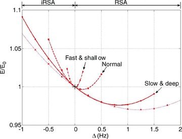
Simulations are performed with the Ben-Tal (2006) model, using prescribed HR functions. Positive Δ represents RSA, negative Δ represents inverse RSA, constant heart rate is marked by a cross at Δ= 0. E/E₀ curves are plotted as functions of Δ (E is calculated with eqn (5), E₀ is the value of E at Δ= 0), constraining the partial pressure of CO₂ along each curve. Data points are obtained from the simulation, and the continuous lines are least-squares quadratic fits. Data points represented by circles (fitted with a continuous line) were taken with T= 10 s, V_T= 1.0 l, constraining the averaged arterial partial pressure of CO₂ to 38.7124 mmHg and normalizing E by 39.98 Hz. Squares with a dashed line were taken with T= 5 s, V_T= 0.5 l, constraining the averaged arterial partial pressure of CO₂ to 38.5611 mmHg and normalizing E by 4.968 Hz. Diamonds with dashed–dotted line were taken with T= 2.5 s, V_T= 0.25 l, constraining the averaged arterial partial pressure of CO₂ to 38.5004 mmHg and normalizing E by 0.2225 Hz. Triangles with a dotted line were taken with T= 10 s, V_T= 1.08 l, constraining the averaged arterial partial pressure of CO₂ to 38.5995 mmHg and normalizing E by 62.482 Hz.

Figure 11. Insignificant energy saving when O₂ is constrained.

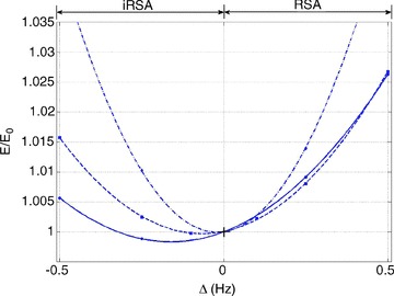
Simulations are performed with the Ben-Tal (2006) model, using prescribed HR functions. Positive Δ represents RSA, negative Δ represents inverse RSA, constant heart rate is marked by a cross at Δ= 0. E/E₀ curves are plotted as a function of Δ (E is calculated by eqn (5), E₀ is the value of E at Δ= 0), constraining the partial pressure of O₂ along each curve. Data points are obtained from the simulation, and the continuous lines are least-squares quadratic fits. Data points represented by circles (fitted with a continuous line) were taken with T= 10 s, V_T= 1.0 l, constraining the averaged arterial partial pressure of O₂ to 105.7143 mmHg and normalizing E by 13.2576 Hz. Squares with a dashed line were taken with T= 5 s, V_T= 0.5 l, constraining the averaged arterial partial pressure of O₂ to 105.8179 mmHg and normalizing E by 4.974 Hz. Diamonds with dashed–dotted line were taken with T= 2.5 s, V_T= 0.25 l, constraining the averaged arterial partial pressure of O₂ to 105.1352 mmHg and normalizing E by 1.069 Hz.

In Fig. 11 RSA does not give an energy advantage under any breathing regime (there is an insignificant reduction in energy for inverse RSA when breathing is slow and deep). This result is in agreement with our calculations in part I and further support the hypothesis (see Discussion below).

Figure 12 summarizes the second set of experiments and shows / and / as a function of Δ for both humans and dogs, under three breathing patterns (normal, fast and shallow, and slow and deep) and three mean HR values (low, normal HR and high). The particular values differ between humans and dogs (e.g. what is meant by ‘normal’ HR). Gas exchange efficiency improves with slow and deep breathing and with increased mean HR but this change is hardly affected by Δ (nevertheless, we can see a very small improvement when Δ is increased). This is consistent with the experimental results of Sin et al. 2010. Figure 12 also shows that the results for dogs and humans are qualitatively the same although the changes in / as a function of Δ are more visible for dogs.

Figure 12. Gas exchange efficiency improves with slow and deep breathing and with increased mean heart rate but this is unrelated to RSA.

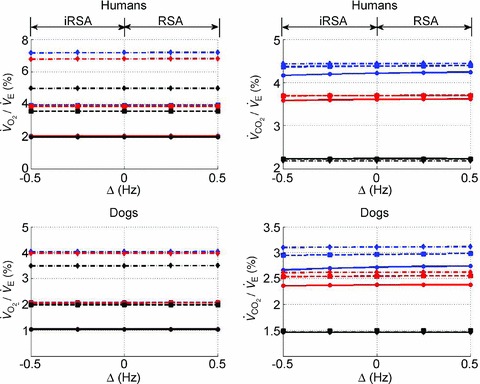
Volumes of O₂ (left panels) and CO₂ (right panels) taken up or removed by the blood over a minute normalized by the minute ventilation and converted to percentage, calculated with prescribed heart rate functions (shown in Fig. 8). Upper panels are done with human parameters, and for these, data in dark grey (blue online) have T= 10 s, V_T= 1 l, data in light grey (red online) have T= 5 s, V_T= 0.5 l, and data in black have T= 2.5 s, V_T= 0.25 l. The minute ventilation was the same for all these simulations: V_T/T= 0.1 l s⁻¹= 6 l min⁻¹. Data represented by circles connected with a continuous line have m= 0.6 Hz, squares with dashed line have m= 1.2 Hz, and diamonds with dashed–dotted line have m= 2.4 Hz. Lower panels are performed with dog parameters, and for these, data in dark grey (blue online) have T= 8 s, V_T= 0.42 l, data in light grey (red online) have T= 4 s, V_T= 0.21 l, and data in black have T= 2 s, V_T= 0.105 l. The minute ventilation was the same for all these simulations: V_T/T= 0.1 l s⁻¹= 3.15 l min⁻¹. Data represented by circles connected with a continuous line have m= 0.5 Hz, squares with dashed line have m= 1.0 Hz, and diamonds with dashed–dotted line have m= 2.0 Hz. All other parameters are given in Appendix A.

Discussion

The physiological function of RSA is studied theoretically in this paper for the first time. The study was performed in two parts. First, the optimal HR was calculated using techniques from optimal control theory. Second, the HR function was prescribed and the cardiac work, as well as the volumes of O₂ and CO₂ taken up or removed by the blood, respectively, were calculated. The calculations in each part of this study were performed using different mathematical techniques and slightly different models, yet they give consistent results. Here, we discuss important novel features of our study and compare them with published animal and humans experiments.

The physiological significance of RSA

In this study we proposed a new hypothesis for the physiological function of RSA – that RSA minimizes the work done by the heart while maintaining a desired average partial pressure of CO₂. We compared it with the previously suggested hypothesis that RSA optimizes gas exchange efficiency by matching ventilation and perfusion in the lungs (Hayano et al. 1996; Yasuma & Hayano, 2004; Sin et al. 2010). In the first part of our study we showed that, using a simple model, the new hypothesis can be defined precisely and solved as an optimization problem while the previous hypothesis cannot. In the second part of our study we conducted a series of numerical experiments on a more physiologically realistic model (Ben-Tal, 2006) and showed that gas exchange efficiency improved with slow and deep breathing and with increased mean HR but that this was unrelated to RSA. This result is consistent with Sin et al. (2010) but distinct to Hayano et al. (1996). Our numerical experiments support the new hypothesis that RSA minimizes the work done by the heart while maintaining a desired average partial pressure of CO₂ (as shown in Fig. 10 for linearly increasing and linearly decreasing HR and in Supplementary Fig. S3, for sinusoidal HR). One might argue that the idea of energy saving due to RSA is not new. It has been suggested before (Yasuma & Hayano, 2004; Sin et al. 2010) that RSA decreases the energy expenditure of the cardiopulmonary system by matching ventilation to perfusion, and that the association between low heart rate variability and increased cardiac mortality is due to diminished cardiac energy efficiency. However, our hypothesis is different in that it emphasizes the need to maintain certain levels of blood partial pressure of CO₂ rather than to match ventilation and perfusion and it has been substantiated by calculations using optimal control theory and numerical simulations in several models.

Our calculations gave an energy saving of 3% (calculated over one breath) of the work done by the heart. This translates to a saving of at least 35 cal h⁻¹ (at rest, an average person consumes about 70 kcal h⁻¹; 1/6 of this is used by the heart and 10% of the energy used by the heart is translated into cardiac output; Vogel, 1992). This gives an estimate of 1.16 kcal h⁻¹ for the work done by the heart at rest, and 35 cal h⁻¹ saving due to RSA). Note that in our model we found that under slow and deep breathing the energy required to maintain the same levels of CO₂ as under normal breathing is higher. To put this saving in perspective, 35 cal = 146.5 Joules which is equivalent to about four punches delivered each by a 3 kg mass moving at 5 m s⁻¹. It might mean that RSA gives an evolutionary advantage. Energy saving due to RSA might also explain why chronic vagal nerve stimulation improves heart function (De Ferrari et al. 2011).

Controlling blood partial pressure: CO₂versus O₂

When we defined the optimization problem we had to introduce the constraint that the blood partial pressure of CO₂ (or O₂) has a given value on average (over one breathing period). Without this constraint the optimization problem cannot be solved mathematically because there could be more than one solution that satisfies the other two constraints (i.e. satisfies the model differential equations and the steady state requirement). Alternatively, one could have specified an initial value for the blood partial pressure or the alveolar partial pressure but this makes less sense physiologically for reasons we discuss below. The solution of the uncoupled systems (Models 1a and 1b) required the specification of the blood partial pressures of both O₂ and CO₂. However, once O₂ and CO₂ are coupled, only the partial pressure of one of them can be specified – constraining both partial pressures is impossible mathematically (except in the particular case when the solution is known in advance). We calculated the optimal HR in part I of our study and conducted the numerical experiments in part II for both cases – once when the partial pressure of CO₂ was constrained and once when the partial pressure of O₂ was constrained. We found that constraining CO₂ gave stronger RSA in part I of the study and a greater energy saving in part II. This is consistent with several physiological observations as we now discuss:

1. CO₂ is the primary substance affecting the chemical control of breathing at rest and at sea level (Guyton & Hall, 2000) – small deviations from normal levels of CO₂ in the blood have an immediate effect on ventilation, while levels of O₂ in the blood need to drop by a relatively larger amount before ventilation is affected. It therefore makes sense physiologically to constrain the average value of the blood CO₂ partial pressure rather than the O₂ partial pressure.

2. Tzeng et al. (2007) measured RSA in spontaneously breathing humans under hypercapnia, hypoxaemia and control. They found that hypercapnia, not hypoxaemia, was associated with an increase in RSA amplitude.

3. Kotani et al. (2000) measured RSA in paced breathing human subjects and monitored the end-tidal CO₂ partial pressures. They reported that these partial pressures were maintained at their eucapnic values.

The last two observations support our hypothesis that one of the functions of RSA is to maintain physiological levels of arterial CO₂.

The optimized HR function

The time-dependent changes of the HR calculated in part I of our study are similar to measurements by Taha et al. (1995). The time-dependent changes in the R-R interval (obtained by plotting the inverse of the HR function) look similar to measurements of RSA reported in Suder et al. (1998), Kotani et al. (2000), Tzeng et al. (2007) and Kotani et al. (2008). Interestingly, the initial increase in the R-R interval (which corresponds to a decrease in HR during inspiration) seen in Fig. 3 was also reported in Suder et al. (1998) and is seen in some cases in Kotani et al. (2000), Tzeng et al. (2007) and Kotani et al. (2008). In some plots of the HR function (Figs 4–6), an initial decrease in the HR (which corresponds to the initial increase in R-R interval) gets stronger with increased RSA. In our calculations the minimum of the R-R interval function occurs toward the end of inspiration similar to Kotani et al. (2000) and Kotani et al. (2008) but unlike Tzeng et al. (2007), where the minimum occurs slightly later during expiration. The amplitude of RSA in Fig. 3 is about 1.5 s. This is similar to the values reported in the literature: 2.5 s in Suder et al. (1998) and 0.8 s in Kotani et al. (2008).

The time-dependent changes in HR (or R-R interval) did not change qualitatively when calculated using three different models (Fig. 3), different inspiration/expiration ratios (Fig. 7) and different expressions for the work done by the heart (Fig. 13).

Mean HR and RSA

In all the calculations shown in the present study we found that increased mean HR was associated with increased RSA. This was the case when the pattern of breathing was changed while keeping the minute ventilation the same (part I and part II), when increasing the required average value of the blood CO₂ partial pressure in the constraint (part I) and when increasing the tidal volume while keeping the breathing frequency the same (part I). All these observations could be understood intuitively when thinking about the hydrodynamic analogy (and reversing the flow direction): an increase in the amount of CO₂ that leaves the lungs over one breathing period will require an increase in the inflow (and therefore an increase in HR) if the average levels of CO₂ in the blood are to stay the same (or alternatively if the average blood levels of CO₂ increase but the amount of CO₂ that leaves the lungs stays the same). The association between increased mean HR and increased RSA is consistent with Tzeng et al. (2007) who measured the effect of hypercapnia on spontaneously breathing humans and reported that “the RSA amplitude increase was associated with a paradoxical rise in HR” as well as an increase in tidal volume. The response to hypercapnia in humans (Sasano et al. 2002) when the tidal volume and frequency were unchanged showed an increase in RSA amplitude with increased hypercapnia but a decrease or no change in mean HR. In contrast, in our model, we see a decrease in both mean HR and RSA under hypercapnia (this response is qualitatively similar to the response seen in our model when the amplitude of q_in is reduced so is not shown here). We believe that this difference in the results may be explained by an absence of feedback mechanisms including peripheral and central chemoreceptors in our model and is the subject of a future study.

Ventilation pattern and RSA

Our calculations in both parts of the study show an increase in RSA under slow and deep breathing (compared with fast and shallow breathing when minute ventilation is fixed) or under increased tidal volume (when the breathing frequency is fixed). This is consistent with several human experiments (Hirsch & Bishop, 1981; Taha et al. 1995; Sin et al. 2010).

Humans versus dogs

To eliminate the possibility that the controversy over gas exchange efficiency is due to species differences, we repeated some of our calculations using dog parameters (given in Appendix A). We did not find qualitative differences between dogs and humans. In both cases, gas exchange efficiency improved with slow and deep breathing and with increased mean heart rate but this was unrelated to RSA.

Sensitivity to changes in parameters

It is important to emphasize that we did not fit any of the parameters to get the results we show in this study. The parameters are typical and were obtained based on physiological, independent measurements. Since it is expected that the parameters will vary from person to person and over time, we checked the sensitivity of the results for Model 1b to changes in parameters by changing the five non-zero parameters in eqn (3) (D₁, D₂, Aα₂, Bβ₁, Bβ₂). The first three of these were varied by ±10%, and the last two by ±1%. Since each of these parameters represents a combination of physiological values, this tests a wide range of possibilities. We found that our results are robust with respect to changes in parameters (see Supplementary Fig. S5). We also repeated our calculations in part I of the study using dog parameters and found the same trends (see Supplementary Figs S6–S10).

Limitations of the study

The mathematical models we used are crude simplifications of reality. Some of the limitations of the reduced models derived in part I of the paper have already been pointed out – averaging the blood partial pressures over the heart beats led to a difference of about 10 mmHg between p_ao and , which is not physiologically realistic but consistent with another model of this kind (Topor et al. 2004). This limitation, however, does not exist in part II of our study. Other important limitations were that the lung is represented by a single container, the physiological and anatomical dead spaces are lumped together and that CO₂ binding to haemoglobin is not taken into account. We found, however, that the results are robust with respect to shifts in the haemoglobin saturation curve (see Supplementary Fig. S1). The models we used do not include any feedback mechanisms. This made it easier to explore the physiological function of RSA, without complicating matters with the question of how RSA is produced (centrally generated and reflexively evoked RSA; Anrep et al. 1936). A feedback mechanism is expected to affect the shape of the respiratory pattern, so we calculated the optimal HR for two other respiratory patterns. We found that while there is a shift in the maximum value of the HR, RSA persists (see Supplementary Fig. S2). All these limitations could explain why some of our computational outputs do not match all experimental observations quantitatively. For example, the RSA amplitude is too large in some of our calculations and the mean HR seems too low when the optimal calculation is done using Model 1b. Nevertheless, the models we used are based on the main physiological principles that drive the system and could therefore provide new insight into the physiological function of RSA. Our study predicted correctly several trends seen experimentally and these trends persisted under changes in parameters, in the definition of the energy function, in shifts of the haemoglobin saturation curve and in inputs pattern (of both HR and respiration).

Conclusions

We conducted a theoretical study of the physiological function of RSA by formulating an optimization problem and calculating the optimal HR function using techniques from optimal control theory and by numerical simulations of simplified models of gas exchange. Our study led us to propose a new hypothesis for the physiological function of RSA – that RSA minimizes the work done by the heart while maintaining a desired average partial pressure of CO₂. This new hypothesis needs more verification by mathematical models that take more physiological details into account as well as by further in vivo experimental studies.

Glossary

Abbreviations

HR

heart rate

RSA

respiratory sinus arrhythmia

Appendix A

Variables and parameters

Table 2 gives a list of most of the parameters encountered in the paper; those that are not mentioned here are defined in Appendix B. These parameters are typical for humans and dogs (i.e. represent an average subject) and are used as the default if an explicit value is not mentioned when specific results are presented. All human values are taken from Ben-Tal, 2006.

Table 2.

Default parameter values for humans and dogs

Parameter	Meaning	Units	Human value	Dog value (reference)
Pm	Atmospheric pressure	mmHg	760	760
Vo	Mean alveolar volume	l	2.5	0.530 (Stahl, 1967)
Cu	Unit conversion factor	l mol−1	25.426	25.507 (calculated at 38°C)
TL	Heart beat period	s	60/72	60/70 (Hayano et al. 1996)
Pw	Water vapour pressure at body temperature	mmHg	47	49.750 (Lemmon, 2011)
fom	Dry atmospheric O2 fractional concentration		0.21	0.21
fcm	Dry atmospheric CO2 fractional concentration		0	0
VT	Tidal volume	l	0.4	0.21 (Hayano et al. 1996)
VD	Dead-space volume	l	0.15	0.07 (calculated as VT/3)
Vc	Capillary volume/heart stroke volume	l	0.07	0.014 (Hayano et al. 1996)
R	Airway resistance to flow	mmHg s−1 l−1	1	1.6 (Stahl, 1967)
E	Lung elastance	mmHg l−1	2.5	14 (Stahl, 1967)
T	Respiratory period	s	5	4 (Hayano et al. 1996)
ω	Respiratory angular frequency	rad s−1	2π/5	2π/4 (Hayano et al. 1996)
Do	O2 diffusion capacity	l mmHg−1 s−1	3.5×10−4	2.7×10−4 (Jouasset-Strieder et al. 1966)
Dc	CO2 diffusion capacity	l mmHg−1 s−1	7.08×10−3	5.462×10−3 (calculated as 20.22*Do)
σ	O2 solubility in blood plasma	mol l−1 mmHg−1	1.4×10−6	1.4×10−6
σc	CO2 solubility in blood plasma	mol l−1 mmHg−1	3.3×10−5	3.3×10−5
Th	Capillary haemoglobin concentration	mol l−1	2×10−3	2.283×10−3 (Hayano et al. 1996)
KT	Equilibrium constant in haemoglobin saturation function	l mol−1	104	104
KR		l mol−1	3.6×106	3.6×106
L			1.712×108	1.712×108
h	Capillary H+ ions concentration	mol l−1	10−7.4	10−7.4
r2	Dehydration reaction rate	s−1	0.12	0.12
l2	Hydration reaction rate	l s−1 mol−1	1.64×105	1.64×105
δ	Reaction rate acceleration factor due to catalysing enzyme		101.9	101.9

The values of p_o, p_c and z (the blood partial pressure of O₂, the blood partial pressure of CO₂ and the concentration of HCO₃⁻, respectively) were initialized every heart beat when the Ben-Tal (2006) model was solved. These values were taken as p_o= 40 mmHg (for humans) and 36 mmHg (for dogs; Calder, 1981), p_o= 46 mmHg (for humans) and 42 mmHg (for dogs; King, 2003) and for both species.

All the values for dogs were obtained at a body mass of 17.5 kg. When a reference is not given for dog values, that parameter is assumed to be the same as for humans.

Appendix B

Full model equations

Here we list the equations of the full model for convenience. See Ben-Tal (2006) for a full derivation and discussion of the model dynamics.

(1B)

(2B)

(3B)

(4B)

(5B)

(6B)

where:

(7B)

(8B)

(9B)

(10B)

(11B)

(12B)

(13B)

Here t is time, P_A is the alveolar total pressure, P_L is the pleural pressure, f_o is the concentration of O₂ in the alveoli, f_c is the concentration of CO₂ in the alveoli, p_ao is the alveolar partial pressure of O₂, p_ac is the alveolar partial pressure of CO₂, p_o is the blood partial pressure of O₂, p_c is the blood partial pressure of CO₂, z is the concentration of HCO₃⁻¹, V_A is the lung volume, q is the air flow, q_in is the inspired airflow and is the haemoglobin saturation function. f_oi and f_ci are the inspired fractional concentration of O₂ and CO₂, respectively. f_oi is calculated as follows (for the calculation of f_ci replace o by c):

(14B)

where f_od is the alveolar concentration of O₂ at the end of expiration. The meaning of all the other symbols as well as their values and units are listed in Appendix A.

The blood variables p_o, p_c and z are reset to venous blood values after every time interval T_L, which is the transient time of blood in the lungs and is also assumed to be the time between heart beats.

Appendix C

Full model reduction

In this appendix we show how Model 1a, Model 1b, Model 2 and Model 3 were derived from the full model described in Appendix B.

Model 1a

By differentiating both sides of eqn (11B) with respect to time we get:

(2C)

By assuming that D_c(p_c−p_ac) =−D_o(p_o−p_ao) (i.e. the respiratory exchange ratio is one), and by linearizing eqn (1B) near the equilibrium point P_A=P_m we get (Ben-Tal, 2006):

(3C)

Since P_L(t) is a given function (see Appendix B), eqn (3C) can be solved directly. This leads to the steady-state solution:

(4C)

which can be used to find a solution for V_A:

(5C)

We now assume that the oscillations in P_A and V_A are relatively small (P_m= 760 mmHg while mmHg and V_o= 2.5 l while V_T/2 = 0.2 l under normal conditions) and that therefore P_A≍P_m and V_A≍V_o. This means that the term in eqn (2C) can be ignored. Using this, eqn (2B) and the assumption that the respiratory exchange ratio is one we get:

Assuming that V_T≥V_D, that f_od≍f_o and rearranging eqn (14B) gives

By rearranging eqn (11B) we can express f_o as a function of p_ao and arrive at the equation:

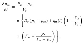(6C)

Now we need to simplify the equation for p_o. We begin by rearranging eqn (4B) and noticing that . This gives:

We now integrate both sides of the equation from 0 to T_L (the time between heart beats) and divide both sides by T_L. We then make the assumption that p_ao does not change much during this short period of time and can be treated as a constant for the duration of the interval. This leads to the following equation:

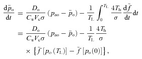where . By taking HR(t) = 1/T_L we get the second equation for Model 1a. Note that the difference between the saturation values at the start and end of the capillaries, , can be approximated by a constant under normal conditions.

A similar integration process for eqn (6C) leads to the first equation for Model 1a:

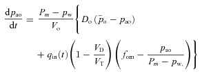Model 1b

By differentiating both sides of eqn (12B) and making the same assumptions as before (that in steady state, P_A≍P_m and V_A≍V_o, and that the exchange ratio is one, we get:

Using eqns (3B) and (14B) for CO₂, realizing that f_cm= 0, replacing f_cd by f_c, expressing f_c through P_ac, averaging both sides of the equation and assuming that p_ac is much slower than p_c, we get the first equation for Model 1b:

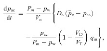where

To get the second equation for Model 1b, we first couple eqns (5B) and (6B):

We then average both sides of the equation and assume that p_ac is much slower than p_c. This leads to:

where HR (t) = 1/T_L and

We also assume that most of the time (this is a reasonable assumption given the value of the reaction rate acceleration factor δ). We can therefore express z as a function of p_c: . We further assume that and we arrive at the second equation for Model 1b:

where p_c(0) is a constant (usually chosen as 46 mmHg).

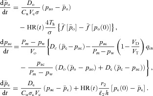
Model 2

In Model 2 we relax the assumption of a constant respiratory exchange ratio but we keep all the other assumptions and approximations the same. This leads to the following four equations:

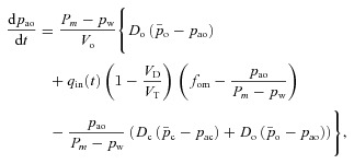Model 3

In Model 3 we allow the alveolar pressure and the lung volume to oscillate but keep all the other assumptions the same as in Model 2. This leads to the following equations (note that we now need to add the right term in eqn (2C)):

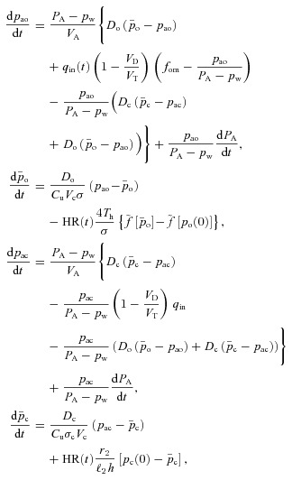where P_A and V_A are approximated by eqns (4C) and (5C) (one could instead add a fifth differential equation, eqn (1B), which will give an accurate solution for P_A and V_A).

Appendix D

Solution of the optimal control problem

In this appendix we first show how the optimal control problem for Models 1a and 1b is solved. We then describe some of the optimal control theory needed to justify the solution. Recall that Model 1a and Model 1b can be written more simply as:

(D1)

The optimal control problem is to find u(t) such that is minimized subject to the following constraints:

1. The differential eqns (D1) are satisfied.

2. The system is in steady state. That is, and

3. h₂ has a given value on average. That is, where is a constant.

By using the Fundamental Theorem of Calculus, the third constraint can be written as the differential equation

(D2)

with the boundary conditions

We now construct a new quantity (called the Hamiltonian):

where and are some functions of time to be determined (called the Lagrange multipliers) and the derivatives dh₁/dt, dh₂/dt and dx/dt are given by eqns (D1) and (D2). We then calculate the derivatives , , and and use them to construct three additional differential equations:

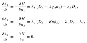(D3)

By setting we can find which can then be substituted into eqns (D3) and (D1).

We now have six differential eqns (D1), (D2) and (D3) which need to be solved simultaneously. To do that we need six boundary conditions. These are: (1) h₁(0) =h₁(T), (2) h₂(0) =h₂(T), (3) x(0) = 0, (4) , (5) and (6) . We solved this system of equations numerically by using the bvp4c subroutine in MATLAB.

Optimal control theory

The first four boundary conditions described above have been defined by the problem. The last two were added by us. To better explain why we made this choice of boundary conditions we need to give some background on the theory that leads to the equations constructed above. The derivation below is based on Lenhart & Workman (2007) and is done for one state variable, x(t). The control problem is to find u(t) such that is minimized while still satisfying the differential equation (this is the constraint).

We assume that the optimum exists, denote it by and let be the corresponding solution of the differential equation (that is, the solution obtained when ). Let h(t) be some arbitrary ‘variation’ function, and ɛ some small real number. Any non-optimal u(t) can then be written as and the corresponding solution of the differential equation can be regarded as . Let be some unknown function. We observe that:

and that therefore

This means that:

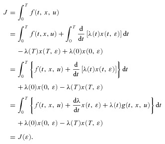Recall that by assumption, and is an optimal pair at and that therefore is optimized at when

Differentiating with respect to gives

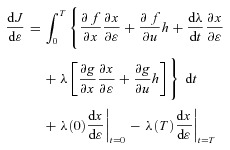and after rearranging the terms and setting we get:

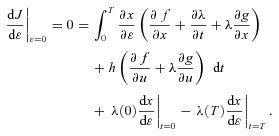(D4)

For eqn (D4) to be satisfied the following conditions are required:

1.

2.

3. = 0, where

The first two conditions lead to the construction of an additional differential equation (when there is more than one state-variable, a similar procedure will lead to the construction of more differential equations, see for example eqn D3). If x(0) is a given number, (that is, no variations are allowed – the optimal solution is required to satisfy the given boundary condition) and can be free (that is, its value can come out of the calculation). If x(0) is free, needs to be set to zero. Similarly for x(T): if it has a given value, is left free, if x(T) is free, needs to be set to zero. This was the case for boundary conditions 3 and 4 in the example above. However, when the boundary conditions are periodic as is the case for boundary conditions 1 and 2 in the example above, we can no longer say that the variation at the boundary is zero (because we do not know what the exact value is, it has to be the result of the optimal calculation and therefore be allowed to vary). We can, however, expect that because the solution is periodic and smooth and therefore require that as we did for boundary conditions 5 and 6 in the example above.

Author contributions

A.B.-T.: mathematical model development, idea conception, writing and editing the manuscript. S.S.S.: numerical simulations, preparation of figures, producing the first draft of the manuscript. J.R.F.P.: idea conception, physiological content, editing the manuscript. All authors approved the final version.

References

- Anrep GV, Pascual W, Rossler R. Respiratory variations of the heart rate. II. The central mechanism of the respiratory arrhythmia and the inter-relations between the central and the reflex mechanisms. Proc Royal Soc Lond B Biol Sci. 1936;119:218–230. [Google Scholar]
- Batzel JJ, Schneditz D, Tran TH. Cardiovascular and Respiratory Systems: Modeling, Analysis, and Control. Philadelphia: Society for Industrial and Applied Mathematics; 2007. [Google Scholar]
- Ben-Tal A. Simplified models for gas exchange in the human lungs. J Theor Biol. 2006;238:474–495. doi: 10.1016/j.jtbi.2005.06.005. [DOI] [PubMed] [Google Scholar]
- Calder WA., 3rd Scaling of physiological processes in homeothermic animals. Annu Rev Physiol. 1981;43:301–322. doi: 10.1146/annurev.ph.43.030181.001505. [DOI] [PubMed] [Google Scholar]
- Cheng L, Ivanova O, Fan H-H, Khoo MCK. An integrative model of respiratory and cardiovascular control in sleep-disordered breathing. Respir Physiol Neurobiol. 2010;174:4–28. doi: 10.1016/j.resp.2010.06.001. [DOI] [PMC free article] [PubMed] [Google Scholar]
- De Ferrari GM, Crijns HJGM, Borggrefe M, Milasinovic G, Smid J, Zabel M, et al. Chronic vagus nerve stimulation: a new and promising therapeutic approach for chronic heart failure. Eur Heart J. 2011;32:847–855. doi: 10.1093/eurheartj/ehq391. [DOI] [PubMed] [Google Scholar]
- Giardino ND, Glenny RW, Borson S, Chan L. Respiratory sinus arrhythmia is associated with efficiency of pulmonary gas exchange in healthy humans. Am J Physiol Heart Circ Physiol. 2003;284:H1585–H1591. doi: 10.1152/ajpheart.00893.2002. [DOI] [PubMed] [Google Scholar]
- Grossman P, Taylor EW. Toward understanding respiratory sinus arrhythmia: relations to cardiac vagal tone, evolution and biobehavioral functions. Biol Psychol. 2007;74:263–285. doi: 10.1016/j.biopsycho.2005.11.014. [DOI] [PubMed] [Google Scholar]
- Guyton AC, Hall JE. Textbook of Medical Physiology. Philadelphia: Saunders; 2000. [Google Scholar]
- Hayano J, Yasuma F. Hypothesis: respiratory sinus arrhythmia is an intrinsic resting function of cardiopulmonary system. Cardiovasc Res. 2003;58:1–9. doi: 10.1016/s0008-6363(02)00851-9. [DOI] [PubMed] [Google Scholar]
- Hayano J, Yasuma F, Okada A, Mukai S, Fujinami T. Respiratory sinus arrhythmia. A phenomenon improving pulmonary gas exchange and circulatory efficiency. Circulation. 1996;94:842–847. doi: 10.1161/01.cir.94.4.842. [DOI] [PubMed] [Google Scholar]
- Hirsch JA, Bishop B. Respiratory sinus arrhythmia in humans: how breathing pattern modulates heart rate. Am J Physiol Heart Circ Physiol. 1981;241:H620–H629. doi: 10.1152/ajpheart.1981.241.4.H620. [DOI] [PubMed] [Google Scholar]
- Jouasset-Strieder D, Cahill JM, Byrne JJ. Pulmonary capillary blood volume in dogs during shock and after retransfusion. J Appl Physiol. 1966;21:365–369. doi: 10.1152/jappl.1966.21.2.365. [DOI] [PubMed] [Google Scholar]
- King LG. Textbook of Respiratory Disease in Dogs and Cats. Philadelphia, PA, London: W. B. Saunders; 2003. [Google Scholar]
- Kotani K, Hidaka I, Yamamoto Y, Ozono S. Analysis of respiratory sinus arrhythmia with respect to respiratory phase. Methods Inf Med. 2000;39:153–156. [PubMed] [Google Scholar]
- Kotani K, Takamasu K, Ashkenazy Y, Stanley HE, Yamamoto Y. Model for cardiorespiratory synchronization in humans. Phys Rev E Stat Nonlin Soft Matter Phys. 2002;65:1923–1923. doi: 10.1103/PhysRevE.65.051923. [DOI] [PubMed] [Google Scholar]
- Kotani K, Takamasu K, Jimbo Y, Yamamoto Y. Postural-induced phase shift of respiratory sinus arrhythmia and blood pressure variations: insight from respiratory-phase domain analysis. Am J Physiol Heart Circ Physiol. 2008;294:H1481–H1489. doi: 10.1152/ajpheart.00680.2007. [DOI] [PubMed] [Google Scholar]
- Larsen PD, Tzeng YC, Sin PYW, Galletly DC. Respiratory sinus arrhythmia in conscious humans during spontaneous respiration. Respir Physiol Neurobiol. 2010;174:111–118. doi: 10.1016/j.resp.2010.04.021. [DOI] [PubMed] [Google Scholar]
- Lemmon EW. Vapor pressure and other saturation properties of water. In: Haynes WM, editor. CRC Handbook of Chemistry and Physics. 92nd edn. CRC Press; 2011. pp. 5–6. [Google Scholar]
- Lenhart S, Workman JT. Optimal Control Applied to Biological Models. Boca Raton: Chapman & Hall/CRC; 2007. [Google Scholar]
- Lu K, Clark JW, Jr, Ghorbel FH, Ware DL, Bidani A. A human cardiopulmonary system model applied to the analysis of the Valsalva maneuver. Am J Physiol Heart Circ Physiol. 2001;281:H2661–H2679. doi: 10.1152/ajpheart.2001.281.6.H2661. [DOI] [PubMed] [Google Scholar]
- McGuinness M, Hong Y, Galletly D, Larsen P. Arnold tongues in human cardiorespiratory systems. Chaos. 2004;14:1–6. doi: 10.1063/1.1620990. [DOI] [PubMed] [Google Scholar]
- Paton JFR, Boscan P, Pickering AE, Nalivaiko E. The yin and yang of cardiac autonomic control: vago-sympathetic interactions revisited. Brain Res Brain Res Rev. 2005;49:555–565. doi: 10.1016/j.brainresrev.2005.02.005. [DOI] [PubMed] [Google Scholar]
- Paton JFR, Nalivaiko E, Boscan P, Pickering AE. Reflexly evoked coactivation of cardiac vagal and sympathetic motor outflows: observations and functional implications. Clin Exp Pharmacol Physiol. 2006;33:1245–1250. doi: 10.1111/j.1440-1681.2006.04518.x. [DOI] [PubMed] [Google Scholar]
- Sasano N, Vesely AE, Hayano J, Sasano H, Somogyi R, Preiss D, et al. Direct effect of PaCO2 on respiratory sinus arrhythmia in conscious humans. Am J Physiol Heart Circ Physiol. 2002;282:H973–H976. doi: 10.1152/ajpheart.00554.2001. [DOI] [PubMed] [Google Scholar]
- Shiogai Y, Stefanovska A, McClintock PVE. Nonlinear dynamics of cardiovascular ageing. Phys Rep. 2010;488:51–110. doi: 10.1016/j.physrep.2009.12.003. [DOI] [PMC free article] [PubMed] [Google Scholar]
- Sin PYW, Webber MR, Galletly DC, Ainslie PN, Brown SJ, Willie CK, et al. Interactions between heart rate variability and pulmonary gas exchange efficiency in humans. Exp Physiol. 2010;95:788–797. doi: 10.1113/expphysiol.2010.052910. [DOI] [PubMed] [Google Scholar]
- Stahl WR. Scaling of respiratory variables in mammals. J Appl Physiol. 1967;22:453–460. doi: 10.1152/jappl.1967.22.3.453. [DOI] [PubMed] [Google Scholar]
- Suder K, Drepper FR, Schiek M, Abel HH. One-dimensional, nonlinear determinism characterizes heart rate pattern during paced respiration. Am J Physiol Heart Circ Physiol. 1998;275:H1092–H1102. doi: 10.1152/ajpheart.1998.275.3.H1092. [DOI] [PubMed] [Google Scholar]
- Taha BH, Simon PM, Dempsey JA, Skatrud JB, Iber C. Respiratory sinus arrhythmia in humans: an obligatory role for vagal feedback from the lungs. J Appl Physiol. 1995;78:638–645. doi: 10.1152/jappl.1995.78.2.638. [DOI] [PubMed] [Google Scholar]
- Topor ZL, Pawlicki M, Remmers JE. A computational model of the human respiratory control system: responses to hypoxia and hypercapnia. Ann Biomed Eng. 2004;32:1530–1545. doi: 10.1114/b:abme.0000049037.65204.4c. [DOI] [PubMed] [Google Scholar]
- Tzeng YC, Larsen PD, Galletly DC. Effects of hypercapnia and hypoxemia on respiratory sinus arrhythmia in conscious humans during spontaneous respiration. Am J Physiol Heart Circ Physiol. 2007;292:H2397–H2407. doi: 10.1152/ajpheart.00817.2006. [DOI] [PubMed] [Google Scholar]
- Ursino M, Magosso E. Role of short-term cardiovascular regulation in heart period variability: a modeling study. Am J Physiol Heart Circ Physiol. 2003;284:H1479–H1493. doi: 10.1152/ajpheart.00850.2002. [DOI] [PubMed] [Google Scholar]
- Vogel S. Vital Circuits: On Pumps, Pipes, and the Workings of Circulatory Systems. New York: Oxford University Press; 1992. [Google Scholar]
- Yasuma F, Hayano J-I. Respiratory sinus arrhythmia: why does the heartbeat synchronize with respiratory rhythm? Chest. 2004;125:683–690. doi: 10.1378/chest.125.2.683. [DOI] [PubMed] [Google Scholar]