Reliable evaluation of the quantal determinants of synaptic efficacy using Bayesian analysis

Abstract

Communication between neurones in the central nervous system depends on synaptic transmission. The efficacy of synapses is determined by pre- and postsynaptic factors that can be characterized using quantal parameters such as the probability of neurotransmitter release, number of release sites, and quantal size. Existing methods of estimating the quantal parameters based on multiple probability fluctuation analysis (MPFA) are limited by their requirement for long recordings to acquire substantial data sets. We therefore devised an algorithm, termed Bayesian Quantal Analysis (BQA), that can yield accurate estimates of the quantal parameters from data sets of as small a size as 60 observations for each of only 2 conditions of release probability. Computer simulations are used to compare its performance in accuracy with that of MPFA, while varying the number of observations and the simulated range in release probability. We challenge BQA with realistic complexities characteristic of complex synapses, such as increases in the intra- or intersite variances, and heterogeneity in release probabilities. Finally, we validate the method using experimental data obtained from electrophysiological recordings to show that the effect of an antagonist on postsynaptic receptors is correctly characterized by BQA by a specific reduction in the estimates of quantal size. Since BQA routinely yields reliable estimates of the quantal parameters from small data sets, it is ideally suited to identify the locus of synaptic plasticity for experiments in which repeated manipulations of the recording environment are unfeasible.

recordings of end plate potentials (Fatt and Katz 1952) have shown that stochastic processes underlie the release of neurotransmitters at chemical synapses. Distinct fluctuations in the size of end plate potentials (Del Castillo and Engbaek 1954) reflect a discrete nature in the discharge of neurotransmitters as all-or-none entities or quanta. With the use of Poissonian statistics to model the probability of release (Del Castillo and Katz 1954), the distribution in amplitude could be characterized by assuming that each end plate potential comprises a linear summation of a large number of miniature components of a certain quantal size (Liley 1956) and variability (Boyd and Martin 1956).

Studies in spinal motoneurons, however, have shown disagreement between Poissonian statistics and observed amplitude distributions (Katz and Miledi 1963). Binomial statistics accommodate a finite but estimable number of release sites (Kuno 1964) and improve characterization of the amplitude distribution of inhibitory postsynnaptic potentials of partially deafferented spinal motoneurones (Kuno and Weakly 1972). A similar observation has been made for end plate potentials recorded at newly formed synapses (Bennett and Florin 1974).

Attempts of using binomial statistics (Christensen and Martin 1970) to estimate the number of release sites or release probability required that one or the other was assumed to be constant since the only reliably measurable binomial term was the quantal size (Kuno 1971). Changes to the divalent cation content (e.g., calcium and magnesium) of perfusing solutions permit experimental manipulation of the release probability and have been used to confirm the binomial nature of the amplitude distribution of end plate potentials (Miyamoto 1975). Estimation of the quantal parameters nevertheless poses considerable technical challenges as a result of the difficulty in maximum likelihood estimation of binomial statistics (Robinson 1976).

An alternative approach (Korn et al. 1981) has been applied to goldfish neurones to estimate the quantal parameters using constrained deconvolution. The method has yielded estimates for the number of release sites in agreement with the number of identified presynaptic boutons (Korn et al. 1982). The occurrence of distinctive “quantal peaks” visible in an amplitude histogram (Korn et al. 1987) has rendered the data particularly favorable to the technique (Redman 1990), although their absence does not necessarily preclude its application (Faber and Korn 1988).

Where quantal peaks have been apparent at mammalian central synapses, least squares (Edwards et al. 1990; Stern et al. 1992), maximum likelihood (Liu and Feldman 1992, Stricker et al. 1996), and Gaussian deconvolution (Kullmann and Nicoll 1992; Kullmann 1993) have successfully fitted mixture models to amplitude distributions. In contrast to the peripheral synapses, such peaks are not routinely observed at central synapses (Bekkers 1994) as a consequence of the greater variability in the size of quantal events (Walmsley 1995). Common to all the fitting techniques is that the mixture model of each amplitude distribution is isolated to the data observed at a single release probability.

Modern methods of quantal analysis (Clements and Silver 2000) have thus attempted to circumvent the need to characterize the profile of amplitude distributions by relying solely on the statistical effects of changes in release probability on the first two moments. Such approaches based on multiple probability fluctuation analysis (MPFA) are widely used (Clements 2003) since they are based on fitting a straightforward parabolic relationship between the mean and variance of evoked synaptic responses at different release probabilities (Silver et al. 1998).

An important limitation of methods based on MPFA, however, is their requirement for long recordings from individual cells to acquire substantial data sets to estimate moments accurately and fit their statistical relationships reliably (Silver 2003). Since valid analysis assumes stationarity of electrophysiological conditions and synaptic function, this requirement may confound estimates based on recordings of any considerable duration (Diana and Marty 2003). It is thus desirable and necessary to devise a method to estimate the quantal parameters while obviating such restrictions.

An advantage of modeling amplitude distributions is that the fit is informed by every single observation rather than summarizing each distribution using variance statistics that may carry considerable errors for small data sets. The principal advantage of MPFA, however, is that a single analysis framework can be used to incorporate information from synaptic responses recorded at different conditions of release probability. To date, the respective advantages of the two approaches have remained disunited since the underlying analytical models have generally been thought to be mutually incompatible. Here, we show that this belief is incorrect.

In the present study, we introduce Bayesian Quantal Analysis (BQA) as a novel algorithm to yield accurate estimates of quantal parameters from small data sets of evoked responses that may be observed at different release probabilities. We describe a framework of the algorithm in methods and exemplify an implementation based on binomial statistics. Using simulated data sets of a small size, we benchmark the accuracy of BQA compared with MPFA and challenge the method with realistic complexities characteristic of central synapses. Finally, we validate the results of BQA using experimental data obtained from electrophysiological recordings.

METHODS

Computer simulation and analysis were undertaken using custom software written in Python, incorporating the NumPy and SciPy packages. When we used MPFA, variance-mean analysis was performed as described previously (Silver 2003). The analysis program can be freely downloaded from http://www.ucl.ac.uk/npp/research/mb.

We present the methods in four sections. First, we describe briefly the features of a simple binomial model. In the second section, we consider the use of maximum likelihood estimation to fit amplitude distributions and its intractability for characterization of responses observed at different release probabilities. Third, we show how such data can be analyzed using a Bayesian approach with a detailed description of our particular implementation included in the appendix. Finally, we describe the experimental details of the electrophysiological recordings used for the study.

Binomial modeling.

While our proposed probabilistic approach is not confined to single binomial models, we commence with this simplest case since this facilitates initial description of the method. Consider the probability of release p at each site to conform to a Bernoulli distribution that is identical for all n sites. With the use of a binomial model, the distribution of the number of Bernoulli successes i is described by the binomial probability mass function (i|n, p) where the notation “|n, p” means “given n and p”:

The overall shape of the amplitude distribution of evoked respones x is determined by the binomial probability mass function according to the linear relation x ∞ i. If we define the quantal size q as the constant of proportionality where x = iq, its value would correspond to the fixed distance between adjacent “quantal peaks.” In the binomial model, we assume that the quantal size q and number of release sites n are independent of the probability of release p and mutually independent of each other.

At a given probability of success p, the first moment of a binomial probability mass function (i|n,p) is np. We can thus express the mean response μ of the amplitude distribution of all observations x as a product that scales the first moment by the quantal size

$$\mu =npq$$ (2)

The corresponding variance σ² can be expressed by scaling the second moment np(1 − p) by the squared quantal size np(1 − p)q², With the use of substitution, the variance can be expressed as a quadratic function with respect to the mean μ.

$${\sigma }^2=-\frac{{\mu }^2}{n}+q\mu$$ (3)

For this simplest case, MPFA is performed by fitting a parabola to the statistical relationship of the moment data, using the fitted coefficients to estimate the number of release sites and quantal size. In practice, additional contributions to observed variances arise from sources of variability outside the binomial model. For example, baseline noise confers an additive effect on the variability of the responses, but this is accommodated by subtraction from the observed variances by the known variance of the noise ϵ².

Variability between uniquantal events, however, constitutes a more challenging contribution to observed variances. Furthermore, distinction between intrasite and intersite sources of variance is important for MPFA as it affects the functional form of the relationship between the mean and variance (Silver 2003). Our proposed Bayesian approach, however, does not rely on this functional relationship because the dispersion of observed responses is not summarized using second moment statistics. Instead, we return to the original raw data sets and characterize their distributions using the quantal likelihood function.

Quantal likelihoods.

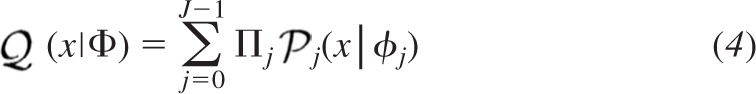
We use the term “quantal likelihood function” to refer to the mixture function (x|Φ) that is selected to describe the profile of the amplitude distribution of evoked synaptic responses x, where the notation “|Φ” means “given the parametric model Φ.” Bayesian approaches have been used previously to develop models to characterize individual amplitude distributions (Turner and West 1993). In the most generic mixture model Φ comprising J components, the profile of jth component is characterized by a probability density function _j(x|ϕ_j) with respect to the parameters ϕ_j. If the magnitude of each component is weighted by a positive coefficient Π_j, such that the weights are distributed according to a probability mass function of unit sum, the quantal likelihood function (x|Φ) can be expressed as a summation.

A previous Bayesian approach (Turner and West 1993) adopted an unconstrained Dirichlet mixture framework with Gaussian component distributions. While the model is flexible, it has not been used widely perhaps because of its conceptual remoteness from biological mechanisms underlying neurotransmitter release limiting intuitive interpretation of results (Bekkers 1994). It is thus desirable to employ a mixture model that characterizes amplitude distributions using a quantal likelihood function that can be expressed with respect to established quantal parameters.

The generic expression in Eq. 4 for the quantal likelihood function can assume any functional form, but a realistic constrained mixture model comprises a minimum of three elements: the probability mass function for the mixture weights Π_j, a probability density function for the baseline noise ₀(x|ϕ₀), and a convolvable probability density function for uniquantal events ₁(x|ϕ₁). While we have chosen an example of each to demonstrate our implementation, BQA is not confined to our selection.

First of all is the discrete distribution that describes the probability of observing i Bernoulli successes from n quantal events, which we have selected as the simple binomial expressed in Eq. 1 by assuming homogeneous release probabilities. An example of a binomial distribution simulating six release sites of release probability 0.35 is illustrated in Fig. 1A.

Fig. 1.

A realistic mixture model to describe the amplitude distribution of evoked responses comprises a minimum of three elements. First, a probability mass function must be assigned for the mixture weights; the example illustrated in A shows a binomial distribution that describes the probability of observing i Bernoulli successes from six release sites each with a release probability of 0.35. The second is the density function used to model baseline noise, such the normal distribution shown in B with a zero mean and a variance of 625 pA² (standard deviation 25 pA). Finally, a probability density function is required to characterize the amplitude distribution of a uniquantal event; here we use a gamma distribution and illustrate an example in C with a gamma shaping parameter of γ = 11.1̄ and gamma scaling parameter of λ = 9 pA, corresponding to a mean quantal size of q = 100 pA since q = γλ. Quantal likelihood function expressed in Eq. 8 combines the three components as illustrated in D (solid line) with the dashed and dotted lines showing the normal and individual gamma components respectively.

The second component is the continuous probability distribution that models background additive noise. For the present implementation, we model its distribution using a bias-free normal probability density function (x|0, ϵ²), where the mean is zero and the variance is ϵ².

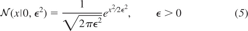An example of a normal probability density function showing bias-free baseline noise of variance 625 pA² (standard deviation 25 pA) is illustrated in Fig. 1B. No attempt is made by the present implementation of BQA to estimate ϵ². In practice, accurate values for the background noise can be readily measured from raw traces. For the purposes of analyzing the computer simulations, we obtain the value for ϵ² directly from the underlying simulation parameters.

Finally, a continuous probability density function must be selected to model the amplitude distribution for a single successful quantal event. Here we use the gamma probability density function (x|γ, λ) expressed with respect to the shaping parameter γ and scaling parameter λ:

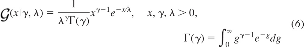where the quantal size constitutes the first moment that can be expressed as the product of the parameters:

$$q=\gamma \lambda$$ (7)

An example of a gamma probability density function (γ = 11.1̄, λ = 9 pA) is illustrated in Fig. 1C. The convolution of multiple identical gamma probability density functions is obtained by simple multiplication of the shaping parameter γ with the number of convolved components. This property allows efficient representation of the effects of combined quantal events as a single summation. We can implement a constrained version of Eq. 4 using a binomial probability mass function to provide discrete weight coefficients to express the quantal likelihood function (x|n, p, γ, λ, ϵ²) with respect to the distribution of overall failures and a summation over an increasing number i of Bernoulli successes.

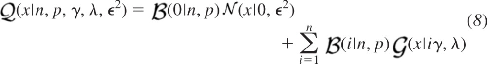An example of the profile of quantal likelihood function combining the elements shown in Figs. 1, A–C, is illustrated in Fig. 1D. While the quantal size q is not included explicitly in Eq. 8, it is represented implicitly by the gamma shaping γ and scaling λ terms according to their product as expressed in Eq. 7. We neglect the additive effects of the background noise on the summation term since they become extremely small with respect to the multiplicative effects of the quantal variability as the number of Bernoulli successes i increases.

If x denotes a vector comprising the observed responses at a fixed release probability p, the joint likelihood can be expressed as a product assuming the data are independent and identically distributed.

The binomial summation in Eq. 8 is discrete, but this does not exclude the use of maximum likelihood estimation to obtains fits to individual amplitude distributions since it can be performed iteratively. Likelihoods are not absolute probabilities, however (Fisher 1922), and therefore do not follow the same basic rules of probability (Fisher 1934). While the product rule for joint probabilities requires only independence of its marginal components, a central tenet of maximum likelihood estimation is a single fixed probability density function to model the data parametrically (Huzurbazar 1948).

Evoked responses observed at different conditions of release probabilities would, however, exhibit dissimilar amplitude distributions and thus violate the prerequisites of maximum likelihood estimation. To accommodate for such differences, we observe that while the numerical value of each likelihood is unnormalized and thus arbitrary, it is proportional to the conditional probability distribution function of the parameters given the data f(Φ|x) (Fisher 1922). If we define c as the constant of proportionality, the likelihood can be scaled to express the conditional probability distribution function.

For evoked responses observed at different release probabilities; however, the magnitude of c will differ for each amplitude distribution. It will not only be affected by the number of observations, but it would also depend on the integral of the likelihood function over the entire set of free parameters over the different release probabilities represented in the data. It would be incorrect to assume c is arbitrarily proportional to the number of data for the corresponding condition of release probability, since the likelihood is a product evaluated by iteration over the same number of observations.

An alternative arbitrary approach would be to assume empirically a constant value for c in attempt to weight the fits of the different amplitude distributions equally. This would, however, bias the estimates towards highly tuned models overwhelmed by perfect fits to only a proportion of the data. Such overfitting characteristically arises from large peaks in likelihood and associated conditional probability density function. Since a large peak in density would occur over a small volume of parameter space, the corresponding mass in probability would be small and thus may represent a highly improbable solution. Moreover for dissimilar amplitude distributions of evoked responses observed at different release probabilities, discrepancies in the regions and volumes of likelihood peaks as well as differences in the likelihood integral in parametric space would confound any attempt of global likelihood evaluation using multiplication and thus preclude valid maximum likelihood estimation. It is therefore unsafe to make any arbitrary assumptions concerning the value of c.

Naïve maximum likelihood estimation using the quantal likelihood function is thus intractable for simultaneous fitting of data that is conditionally partitioned according to different release probabilities. Instead, we undertake the simplest approach by making no arbitrary assumptions concerning the value of c but instead calculate it directly using established terms of probability defined explicitly according to a unified Bayesian framework. While we describe the technique in the next sections, the details of our specific implementation is provided in the appendix.

Bayesian modeling.

Let A and B denote two nominal dichotomous propositions that may be true rather than false according to their corresponding probabilities P(A) and P(B) respectively. We can express the joint probability of both being true P(A, B) with respect the conditional probability P(A|B), which represents the probability of A “given” B is true, using a product according to chain rule.

$$P\left(A,B\right)=P\left(B\right)\times P\left(A|B\right)$$ (11)

where P(B) is called the marginal probability of B since it can be obtained from the joint probability P(A, B) by marginalization of A performed by a summation over all possible outcomes of A according to sum rule.

$$P\left(B\right)={\displaystyle \sum _{A}P\left(A,B\right)}$$ (12)

We can express the joint probability P(B, A) in a similar manner as shown in Eq. 11 by interchanging the terms A and B.

$$P\left(B,A\right)=P\left(A\right)\times P\left(B|A\right)$$ (13)

Since the joint probabilities P(A, B) and P(B, A) mutually correspond, then the right-hand expressions of Eqs. 11 and 13 equate and thus permit expression of one conditional probability with respect to the other.

$$P\left(B|A\right)=\frac{P\left(B\right)\times P\left(A|B\right)}{P\left(A\right)}$$ (14)

Equation 14 is Bayes' rule. In this example above, A and B are binary and thus the possibilities of each comprise two mutually exclusive possible outcomes (i.e., true or false).

Bayesian analysis is based on using Eq. 14 to model the distribution of observed data x with respect to hypothetical parameters ϕ. Since both observed data x and hypothetical parameters ϕ constitute numerical values rather than nominal propositions, we denote their associated probability distribution functions with an f rather than a P, a convention we have observed in Eq. 10. We adopt vector notation for both terms since x may consist of any number of observations and ϕ may comprise more than one parameter. If we replace A with the observed data x and B with the hypothetical parameters ϕ, we can use Eq. 14 to represent a Bayesian model.

$$f\left(\phi |\text{x}\right)=\frac{f\left(\phi \right)\times f\left(\text{x}|\phi \right)}{f\left(\text{x}\right)}$$ (15)

The conditional probability of the data given the parameters f(x|ϕ) represents the likelihood of the observations in the context of the model. It can be calculated in exactly the same way as the likelihood that is maximized during maximum likelihood estimation. For example if the data x are independent and identically distributed, it can be calculated using the product rule as shown in Eq. 9.

The unconditioned probability f(ϕ) constitutes the prior, which refers to probability distribution of the hypothetical parameters in the absence of any data. Priors can be assigned objectively according to the mathematical properties of the parameters. For example, consider a Gaussian model of mean μ and standard deviation σ. While it may be mathematically valid to assign equal probabilities for the mean in the range −∞ < μ < +∞, the same limits cannot be assigned to the standard deviation because its lower bound is zero; in this case a typical Bayesian solution would be to assign equal probabilities in the range −∞ < log(σ) < +∞.

By multiplying the prior by the likelihood, the probability distribution of the parameters in effect is “informed” by the data to yield the probability of the hypothetical parameters given the data f(ϕ|x), or posterior. The remaining denominator term f(x), sometimes called the evidence, represents the probability of the data and constitutes the normalization constant that ensures unity in the integral of the posterior. Analogous to the sum rule expressed in Eq. 12, we can express the probability of the data f(x) with respect to the joint probability of the parameters and data f(ϕ, x) using marginalization. Since the parameters are continuous numerical values rather than nominal propositions, the marginalization is performed by integration rather than summation.

$$f\left(\text{x}\right)={\displaystyle {\int }_{\phi }f\left(\phi ,\text{x}\right)d\phi }$$ (16)

Since according to the chain rule expressed in Eq. 11 the numerator product in the right hand expression of Eq. 15 equates exactly to the integrand of Eq. 16, we can express the normalisation procedure manifestly by substitution.

$$f\left(\phi |\text{x}\right)=\frac{f\left(\phi \right)\times f\left(\text{x}|\phi \right)}{{\displaystyle {\int }_{\phi }f\left(\phi \right)\times f\left(\text{x}|\phi \right)d\phi }}$$ (17)

Consider the posterior f(ϕ|x) to constitute the probability of the two hypothetical parameters ϕ₁ and ϕ₂ given the data i.e., ϕ = (ϕ₁, ϕ₂). Since the posterior is the joint probability distribution f(ϕ₁, ϕ₂|x), we can evaluate the marginal posterior f(ϕ₁|x) for one parameter ϕ₁ by marginalization of the other ϕ₂ using integration.

$$f\left({\phi }_1|\text{x}\right)={\displaystyle {\int }_{\phi 2}f\left({\phi }_1,{\phi }_2|\text{x}\right)d{\phi }_2}$$ (18)

Alternatively we may wish to reparameterize our posterior with respect to new parameters ψ. First we must define our new parameters with respect to our initial parameters according to the invertible functional form ψ = F(ϕ). We can evaluate the transformation in probability space by conditional marginalization using integration over the regions of probability space in which the initial and final parameters are constrained by the functional form ϕ = F⁻¹(ψ).

$$f\left(\psi |\text{x}\right)={\displaystyle {\int }_{\phi =F^{-1}\left(\psi \right)}f\left(\phi |\text{x}\right)d\phi }$$ (19)

For more definitive descriptions of Bayesian modeling, the reader is referred to standard texts detailing probabilistic approaches (Jaynes 2003).

Quantal probabilities.

Let K denote the number of conditions of release probability p_k represented in the data X, where X comprise the K vectors x_k that may differ in number of observations for k = {1, 2, …, K}. The model assumes that the underlying profiles of the amplitude distributions of x_k may differ only as a result of differences in release probability p_k. We represent the family of likelihoods _k as the conditional probabilities of the data x_k given the parameters ϕ_k.

where the terms are subscripted with k, since they may or may not differ according to differences in release probability across the family of likelihoods.

While we have denoted every likelihood term as a conditional probability, each remains arbitrary in numerical value unless multiplied by their respective scalar constant as shown in Eq. 10.

$$f_k\left({\phi }_k|{\text{x}}_k\right)=c_k{f}_k\left({\text{x}}_k|{\phi }_k\right)$$ (21)

Using Bayes' rule, expressed in Eq. 15, we can substitute the constants c_k with the quotient of two unconditioned probabilities.

$$f_k\left({\phi }_k|{\text{x}}_k\right)=\frac{f_k\left({\phi }_k\right)f_k\left({\text{x}}_k|{\phi }_k\right)}{f_k\left({\text{x}}_k\right)}$$ (22)

Equation 22 illustrates that the product of every likelihood f_k(x_k|ϕ_k) with the probability of the parameters in the absence of data f_k(ϕ_k) or prior is proportional to each corresponding conditional probability of the parameters given the data f_k(ϕ_k|x_k) or posterior. The denominator terms f_k(x_k), or evidence, are normalization scalars that can be evaluated by marginalizing the numerator product, as shown in Eq. 17, thus ensuring unity in the integral of each posterior.

$$f_k\left({\phi }_k|{\text{x}}_k\right)=\frac{f_k\left({\phi }_k\right)f_k\left({\text{x}}_{\text{k}}|{\phi }_k\right)}{{\displaystyle {\int }_{\phi k}{f}_k\left({\phi }_k\right)f_k\left({\text{x}}_k|{\phi }_k\right)d{\phi }_k}}$$ (23)

For the present implementation, detailed in the appendix, we use the likelihood function expressed in Eq. 8 and assign priors based on the probabilities of release p_k, the total quantal coefficient of variation ν, and the number of release sites n, i.e., ϕ_k = (p_k, ν, n). To reduce parameter space, we use the known variance of the background noise ϵ² in the likelihood function directly and assume the probability of release p_k is proportional to the mean response μ_k. An advantage of a Bayesian approach is that priors can be assigned that are non informative but nevertheless incorporate knowledge of the means. Due to discrete nature of the integer number of release sites n imposed by our implementation, we sample posterior probability space using a fine grid to perform numerical calculations throughout entire parameter space, a procedure sometimes called “brute-force.”

Since our implementation evaluates posteriors that model probability space with respect to terms that include the release probability p_k, they cannot be combined directly since their parametric models differ according to the differences in release probability represented in the data. Consequently, we change variables to resample posterior probability space using new quantal parameters ψ that are of interest but nevertheless independent of the release probability. If our new parameters can be expressed according to the invertible functional form ψ = F(ϕ), we can evaluate the transformation in probability space by conditional marginalization, as shown in Eq. 19.

$$f_k\left(\psi |{\text{x}}_k\right)={\displaystyle {\int }_{{\phi }_k=F^{-1}\left(\psi \right)}{f}_k\left({\phi }_k|{\text{x}}_k\right)d{\phi }_k}$$ (24)

For the present implementation, detailed in the appendix, our chosen quantal parameters are the quantal size q, the gamma shaping parameter γ, and the maximal response r, i.e., ψ = (q, γ, r). We define the maximal response r as the expected mean response when the probability of release is one (i.e., r = nq). Since none of the parameters are dependent on the release probability and define a common underlying probability density function represented throughout the entire data set , we can express our joint posterior f(ψ|) as proportional to the product of the transformed posteriors.

$$f\left(\psi |\chi \right)\alpha {\displaystyle \prod _{k=1}^K{f}_k\left(\psi |{\text{x}}_k\right)}$$ (25)

We can thus normalize the product to express our joint posterior f(ψ|) and marginalize the result to evaluate the profile of the posterior probability distribution of each parameter given the entire data set. Maximum a posterior, moment-, or median-based measures can be used to obtain best estimates for the quantal parameters, and the cumulative distribution can be sampled at critical intervals to provide confidence limits for each of the quantal parameters. We used the median to obtain the estimates presented in the results. In the appendix, we detail how the analysis was modified to estimate the homogeneity of release probability α by incorporating a beta probability density to model heterogeneous release probabilities.

Electrophysiological recordings.

Spinal cords were extracted from postnatal day (P)12–13 rats as detailed previously (Beato 2008), and 350-μm slices were cut from the lumbar region. All experiments were undertaken in accordance with the Animal (Scientific Procedures) Act (UK) 1986. The extracellular solution used during recordings comprised of artificial cerebrospinal fluid of the following composition (in mM): 124 NaCl, 3 KCl, 25 NaHCO₃, 1 NaH₂PO₄, 2 CaCl₂, 2 MgCl₂, and 11 d-glucose, bubbled with a 95% O₂-5% CO₂ mixture.

Whole cell voltage-clamp patch recordings from motoneurones were performed at room temperature. Electrodes were filled with an internal solution of the following composition (in mM): 140 CsCl, 4 NaCl, 0.5 CaCl₂, 1 Mg₂Cl, 10 HEPES, 5 EGTA, 2 Mg-ATP, 3 QX-314 Br, pH 7.3 with CsOH, and osmolarity of 290–310 mosM. Electrodes were pulled from thick (outer diameter of 1.5 mm and inner diameter of 0.86 mm) borosilicate capillaries (Clarke Biomedical Instruments) to a resistance of 0.5–1 MΩ and fire polished to give a final resistance of 1.5–2 MΩ.

Motoneurones were voltage clamped at −60 mV, and the series resistance of 4–10 MΩ was compensated by 60–80%. Inclusion of CsCl in the intracellular solution resulted in typical input resistance of 40–80 MΩ. The experiment was abandoned if the initial series resistance exceeded 10 MΩ and interrupted if it increased by >20%. The typical whole cell capacitance of ∼200 pF gave a low pass corner frequency of 0.2–0.8 kHz. In all recordings, the voltage error calculated from the maximum current and uncompensated series resistance was <5 mV.

Extracellular stimulation was performed via a patch pipette containing artificial cerebrospinal fluid maneuvered within the ventral region of Rexed lamina VIII. Stimulus trains were used to evoke currents before and after application of 100 μM gabazine (SR-95531, Sigma). The stimulation intensity was gradually increased until a postsynnaptic response was evoked and the stability of the amplitude was ascertained over a range of three to four times the threshold to exclude potential recruitment of additional fibers within a broad range of intensities. If stability could not be obtained, the position of the stimulating electrode was adjusted.

Amplitude measurements of evoked responses were performed as described previously (Silver 2003). Briefly, a 100-μs window centered at the peak of the average response was established to measure the mean deflection for each individual response over this window using as baseline a 1-ms period before the stimulus artifact. The short time constant (200–300 μs) of the stimulus artifact compared with the latency of responses (2–3 ms) precluded interference of amplitude measurements by the capacitative current of the artifact. Amplitude histograms were inspected to confirm that the amplitude of failures were centered at zero.

RESULTS

We present the results in three sections. First, we use computer simulations to compare the performance in accuracy of BQA and MPFA from small data sets. In the second section, we challenge the method with realistic complexities characteristic of central synapses. Finally, we test the performance of BQA using electrophysiological data to determine whether its estimates are consistent with established experimental manipulations.

Comparisons with MPFA.

Accuracy was assessed using computer-generated “experiments” in which the quantal size was always Q = 100 pA and the number of release sites was N = 6 sites, all with identical release probabilities according to a simple binomial model. Gaussian random number generators were used to simulate the baseline noise of standard deviation 25 pA and the variability of quantal size within individual release sites set to a fixed coefficient of variation CV_intra = 0.3. We generated 60 responses for each of only two simulated conditions of release probability.

While fixing the probability of the first condition (P₁ = 0.1), we adjusted the second to assess the effects of a variable range of release probability (0.05 ≤ ΔP ≤ 0.80, increment 0.01) using 100 simulations in each case. Figure 2 illustrates a comparison of the results obtained from MPFA and BQA as pseudocolor histograms smoothed using Gaussian convolution (Bhumbra and Dyball 2010) with 95% confidence limits (i.e., raw 0.025 and 0.975 fractiles) shown in white.

Fig. 2.

Compared with multiple fluctuation probability analysis (MPFA), Bayesian quantal analysis (BQA) yields more accurate estimates of the quantal size q and number of release sites n for small data sets. Computer simulations (q = 100 pA, n = 6 sites, CV_intra = 0.3, baseline noise= 0 ± 25 pA) were used to generate 60 data for each of two conditions of release probability (P₁ = 0.1 fixed, P₂ variable) over a specific range (0.05 ≤ ΔP ≤ 0.8 with increment 0.01). Gaussian-smoothed histograms from 100 simulations illustrate the estimates obtained from MPFA for the quantal size (A) and number of release sites (B) with the 95% confidence limits shown in white (in both plots the y-axis is truncated); corresponding plots for BQA are shown (without truncation) in C and D. Representative examples of mean-variance plots are shown in E (ΔP = 0.2) and F (ΔP = 0.7). The simulated release probabilities and the correct parabolae predicted theoretically from the parameters used for the computer simulations are shown as dotted lines, the best-fit parabolae for MPFA represented as dashed lines, and the parabolae projected by BQA overlayed as solid lines.

At the lowest range in probability, MPFA fails to determine the quantal size (Fig. 2A), whereas the parameter is estimable at greater ranges (e.g., at ΔP = 0.8 the 95% confidence limits are 70.0 pA ≤ q̂ ≤ 131.5 pA). Distributions of the MPFA results for the number of release sites (Fig. 2B) could not be represented graphically without truncation. Estimation is not feasible (e.g., 0.00 sites ≤ n̂ ≤ 21.00 sites, ΔP = 0.2) until ΔP = 0.6 (where 3.40 sites ≤ n̂ ≤ 13.38 sites). BQA results for both quantal size (Fig. 2C) and number of release sites (Fig. 2D) approximate to the correct values. Quantal size is accurately determined throughout (e.g., 90.6 pA ≤ q̂ ≤ 134.6 pA at ΔP = 0.05). While the number of release sites is underestimated at the low extreme in the range of release probabilities, estimation is feasible already at ΔP = 0.2 (2.48 sites ≤ n̂ ≤ 8.29 sites) and more accurate at ΔP = 0.5 (3.83 sites ≤ n̂ ≤ 9.12 sites).

An example of MPFA performed on a simulation over a small range in probability (ΔP = 0.2, P₁ = 0.1, P₂ = 0.3) is shown as a mean-variance graph (Fig. 2E). The theoretically ideal parabola calculated from the underlying simulation parameters is plotted as a dotted line. Since the MPFA solution is a straight line (dashed), it underestimates the quantal size (q̂ = 82.4 pA) and precludes determination of the number of release sites (n̂ = ∞ sites). Results from BQA (projected moment relation shown as a solid line) for the same data, however, are accurate (q̂ = 102.2 pA, n̂ = 5.96 sites). In a second example (Fig. 2F), the large range of simulated release probabilities (ΔP = 0.7, P₁ = 0.1; P₂ = 0.8) imparts curvature to the parabolic fit, but the MPFA estimates (q̂ = 58.3 pA, n̂ = 12.50 sites) are distant from the correct values, while those from BQA are not (q̂ = 97.9 pA, n̂ = 5.97 sites).

Figure 3 illustrates an example of a BQA model based on the data represented in Fig. 2F. For the purposes of illustration, we have marginalized the gamma shaping parameter γ from each posterior f_k(q, γ, r|x_k, μ_k) to allow representation of the posterior distribution for each condition in release probability f_k(q, r|x_k, μ_k) in only two dimensions. Conditional posterior distributions for the quantal size and maximal response are illustrated for the data simulated at a low (P₁ = 0.1; Fig. 3A) and high (P₂ = 0.8, Fig. 3B) release probabilities.

Fig. 3.

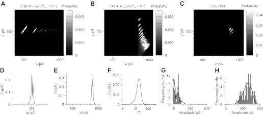
Bayesian quantal analysis combines information from the amplitude distributions of all data from every condition of release probability to yield accurate estimates of the quantal parameters with small data sets (here taken from the data illustrated in Fig. 2F). The conditional posterior distributions for the quantal size q and maximal response r (where r = nq) are illustrated for the data simulated at a low (P₁ = 0.1; A) and high (P₂ = 0.8, B) release probabilities (q = 100 pA, n =6 release sites). With the use of the product rule, the joint posterior distribution for both parameters could be calculated (C) and marginalized by sum rule to evaluate the marginal posteriors for the quantal size (D) and maximal response (E). BQA also characterizes the variability of the quantal events, here using a gamma shaping parameter γ (see text), to allow its estimation from its respective marginal posterior (F). G and H: distribution of the data (bin width = 20 pA) for the two conditions of release probability with their projected profile by the model overlayed a solid line.

Comparison between the two conditional posteriors illustrate five features of BQA for small data sets. Firstly, no single data set from any one condition of release probability permits accurate estimation of both quantal parameters in isolation. Second, data acquired at low release probabilities permit accurate estimation of the quantal size but not the maximal response. Third, the converse is the case at high release probabilities. Fourth, posterior distributions based on binomial models exhibit discrete discontinuities imposed by integer numbers of release sites giving rise to distinct peaks of probability. Finally, each peak reflects the positive linear relationship between the quantal size q and maximal response r given a specific number of release sites n since r = nq.

The joint posterior distribution (Fig. 3C) is constructed using the product rule to combine all probabilistic information from both conditional posterior distributions. With the use of the sum rule, the joint posterior distribution is marginalized in either dimension to evaluate the marginal posteriors for the quantal size (Fig. 3D) and maximal response (Fig. 3E). Marginization of both terms from the original three-dimensional joint posterior evaluates the marginal posterior for the gamma shaping parameter (Fig. 3F).

We evaluate the medians of the marginal posteriors to provide estimates for modeled parameters (q̂ = 97.9 pA, r̂ = 583.9 pA, γ̂ = 17.4) and derived parameters such as the number of release sites (n̂ = 5.97 sites), the quantal coefficient of variation (v̂ = 0.24), and probabilities of release for the two conditions (P̂₁ = 0.090, P̂₂ = 0.867). Histograms of the data simulated at low (Fig. 3G) and high (Fig. 3H) release probabilities show correspondence between their amplitude distributions and their projected profiles according to the model superimposed as black lines.

While the data used for Fig. 2 were generated by simulating only two conditions of release probability, MPFA is routinely performed on experimental results comprising more conditions. We thus assessed the effects of including a third condition by simulating a further 60 observations at the midpoint in release probability within the interval of the other two conditions (Fig. 4, A–D). The additional data, however, results in no obvious improvement in MPFA estimates of the quantal size (Fig. 4A; e.g., at ΔP = 0.8, 64.0 pA ≤ q̂ ≤ 121.5 pA) nor number of release sites (Fig. 4B; e.g., at ΔP = 0.6, 3.71 sites ≤ n̂ ≤ 14.72 sites). There was similarly no obvious amelioration in BQA estimates of the quantal size (Fig. 4C; e.g., at ΔP = 0.05, 89.1 pA ≤ q̂ ≤ 135.0 pA) and number of release sites (Fig. 4D; e.g., at ΔP = 0.5, 3.23 sites ≤ n̂ ≤ 7.91 sites).

Fig. 4.

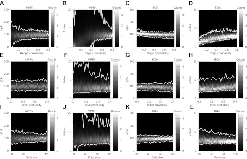
Whereas MPFA requires data sets acquired at high release probabilities or of a large size for accurate estimation of the number of the release sites, BQA does not. Computer simulations (q = 100 pA, n = 6 sites, CV_intra = 0.3, baseline noise= 0 ± 25 pA) were used to generate 60 data for each condition of release probability. Gaussian-smoothed histograms from 100 simulations illustrate the estimates obtained from MPFA for the quantal size (A) and number of release sites (B) with the 95% confidence limits shown in white (in both plots the y-axis is truncated) for data simulated with three conditions of release probability [P1 = 0.1 fixed, P3 = P₁ + ΔP, P₂ = ½(P₁ + P₃)] over a specific range (0.05 ≤ ΔP ≤ 0.8 with increment 0.01). Corresponding plots for BQA are shown (without truncation) in C and D. Using only two conditions (ΔP = 0.5), we assessed the effects of increasing the lower probability (0.10 ≤ P₁ ≤ 0.40, increment 0.01) on MPFA estimates of quantal size (E) and number of release sites (F, truncated) as well as the BQA estimates (G and H). To assess the effects of the data size, the release probabilities for the two conditions was fixed (to P₁ = 0.1 and P₂ = 0.6) while adjusting the size of the data set for each condition (30 ≤ |x_k| ≤ 120, increment 2). Gaussian-smoothed histograms are shown for the MPFA estimates for the quantal size (I) and number of release sites (J, truncated), and for the equivalent plots for BQA (without truncation) in K and L.

For the data illustrated in Fig. 2, the range in release probability simulated was variable, but the lower limit was always fixed (P₁ = 0.1). To assess the converse case, we compared the performance of MPFA and BQA using a fixed range in probability (ΔP = 0.5) while varying the probability for the lower condition (from 0.1–0.4), with a constant number of responses (60) for each of the two conditions (Fig. 4, E–H). At the midtransitional interval (P₁ = 0.25, P₂ = 0.75), the 95% confidence limits for MPFA are wider for both quantal size (Fig. 4E; 63.6 pA ≤ q̂ ≤ 145.2 pA) and number of release sites (Fig. 4F; 3.69 sites ≤ n̂ ≤ 12.19 sites) compared with the BQA estimates (Fig. 4G; 61.0 pA ≤ q̂ ≤ 130.3 pA; Fig. 4H; 3.96 sites ≤ n̂ ≤ 10.69 sites).

Since accurate estimation of moments for MPFA is critically dependent on the data size, we compared the performance of MPFA and BQA while varying the number of simulated responses (from 30–120) for both conditions (Fig. 4, I–L) with a fixed range in release probability to ΔP = 0.5 (P₁ = 0.1; P₂ = 0.6). With only 30 data, the 95% confidence limits for MPFA are wide for both quantal size (Fig. 4I; 55.3 pA ≤ q̂ ≤ 163.0 pA) and number of release sites (Fig. 4J; 2.43 sites ≤ n̂ ≤ 21.00 sites), compared with BQA (Fig. 4K: 65.2 pA ≤ q̂ ≤ 122.6 pA; Fig. 4L; 3.44 sites ≤ n̂ ≤ 11.12 sites).

Comparison of Fig. 4, F and J, illustrates similarities on the effects of increased release probabilities and increased data size on the accuracy of MPFA estimates of the number of release sites. Both a low range in release probability (Fig. 4F) and a minimal size in data sets (Fig. 4J) preclude estimation despite reasonable MPFA results for the quantal size. By contrast, BQA estimation of the number of release sites is feasible throughout the entire range of both manipulations (Fig. 4, H and L).

Realistic complexities.

The performance of BQA was assessed using simulated data in which realistic complexities were introduced while fixing the two conditions of release probability (P₁ = 0.1; P₁ = 0.6), each comprising 60 observations (Fig. 5). Again, we simulated six release sites with a mean quantal size of 100 pA with Gaussian intrasite variability with a coefficient of variation of 30%.

Fig. 5.

BQA is robust to increases in the relative noise and number of release sites. Computer simulations (see Fig. 4) were undertaken with either changes in baseline noise (relative to the quantal size) or number of release sites. Increases in relative noise did not preclude estimation of quantal size (A) and number of release sites (B). Changes in the simulated number of release sites had no discernible effect on the estimated quantal size (C) yet were well detected by BQA (D).

While fixing the quantal size to 100 pA, we investigated the effects of changing the relative baseline noise. Parameter estimation was not precluded by an increased baseline noise up to 64% relative to the quantal size (Fig. 5A; 78.9 pA ≤ q̂ ≤ 188.0 pA; Fig. 5B: 2.22 sites ≤ n̂ ≤ 8.49 sites). For the remaining simulations, the baseline noise was fixed at 25% of the quantal size.

We also assessed whether BQA would successfully detect changes to the simulated number of release sites while maintaining accurate estimation of the quantal size. Increases in the number of release sites did not prejudice BQA estimates for the quantal size (Fig. 5C). Changes in the number of release sites, however, were accurately detected (Fig. 5D): linear regression between the simulated and estimated number of release sites (n̂ = BN + A) yielded 95% confidence limits that spanned one for slope (0.9579 ≤ B ≤ 1.0075) and zero for the intercept (−0.1056 ≤ A ≤ 0.3743).

Central synapses characteristically exhibit considerable variability in the magnitude of uniquantal events. Consequently, we assessed the effects of increases in the variability of quantal events arising from both intrasite and intersite sources (Fig. 6). Intrasite variability was modeled using a Gaussian model for the quantal sizes. Low intrasite variability improved the accuracy of estimates of the quantal size (Fig. 6A) and number of release sites (Fig. 6B). Increases in the coefficient of variation up to 64% did not unduly affect BQA estimates of the quantal size (82.1 pA ≤ q̂ ≤ 142.0 pA) or number of release sites (3.31 sites ≤ n̂ ≤ 10.63 sites) yet were successfully detected by the analysis (Fig. 6C). BQA estimates of the quantal coefficient of variation were overestimated at the low extreme of intrasite variability because the effect of a baseline noise of 25% on uniquantal amplitude distributions was not explicitly included in this BQA implementation.

Fig. 6.

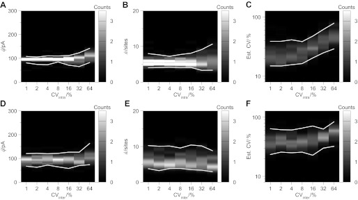
BQA is robust to sources of variability in quantal events. Computer simulations (see Fig. 4) were undertaken with either changes in the intrasite coefficient of variation (Gaussian distributed) or intersite coefficient of variation (gamma-distributed, superimposing a preexisting Gaussian intrasite coefficient of variation of 30%). While very low intrasite coefficients of variation improved the accuracy of estimates of the quantal size (A) and number of release sites (B), estimates were robust with high variability. Changes in intrasite variability were detected by BQA estimates (C). Increases in intersite variability (superimposing a 30% intrasite variability) had no discernible effect on the estimated quantal size (D) and number of release sites (E) yet they were detected by BQA (F).

While fixing an intrasite coefficient of variation to 30%, we assessed the effects of a superimposed intersite variability using a gamma model. Simulated increases in the intersite variability similarly did not adversely affect BQA estimates of the quantal size (Fig. 6D) or number of release sites (Fig. 6E) and again were detected by the analysis (Fig. 6F). At the low extreme of intersite variability, BQA estimates predominantly reflected the fixed intrasite coefficient of variation of 30%.

Central synapses may exhibit heterogeneous probabilities of release across different release sites. Consequently, we generated data in which release sites were simulated to exhibit heterogeneous probabilities of release distributed according to a beta probability mass function of homogeneity α (where increasing α represents greater homogeneity) for three conditions (P̄₁ = 0.1, P̄₂ = 0.5, P̄₃ = 0.9) each comprising 60 observations. The intermediate condition in release probability was included because the amplitude of observed responses would be most dramatically affected by the heterogeneity in the release probabilities for this transitional state.

Initially, we analyzed the data using a BQA model that assumed homogeneous release probabilities to estimate the quantal size (Fig. 7), number of release sites (Fig. 7B), and quantal variability (Fig. 7C). For the set of simulations at the extreme of greatest heterogeneity (α = 0.2), the näıve model yielded shifted estimates for the quantal size and number of release sites. The results were otherwise accurate (e.g., at α = 0.4: 55.6 pA ≤ q̂ ≤ 104.4 pA, 3.90 sites ≤ n̂ ≤ 7.53 sites).

Fig. 7.

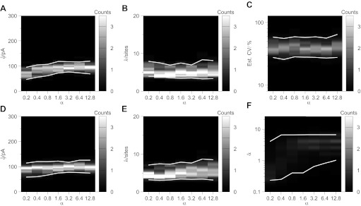
BQA is robust to heterogeneity in the release probabilities across different release sites. Computer simulations (q = 100 pA, n = 6 sites, CV_intra = 0.3, baseline noise= 0 ± 25 pA) were used to generate 60 data for 3 conditions of mean release probability (P₁ = 0.1, P₂ = 0.5, P₃ = 0.9) in which the distribution of probability across release sites conformed to a beta distribution of variable homogenity α. Increases in homogenity showed only marginal effects on the estimates obtained from a BQA model, that assumed homogeneous probability of release, for the quantal size (a), number of release sites (B), and quantal variability (C); effects were minimal from α ≥ 0.4. BQA incorporating a beta probability density function to model heterogeneous probabilities of release yielded accurate estimates for both quantal size (D) and number of release sites (E) throughout the entire range of homogeneity and changes in heterogeneity were detected (F).

The same data were subjected to similar analysis using a BQA implementation that incorporated a beta model (see methods). BQA estimates of the quantal size (Fig. 7D) and number of release sites (Fig. 7E) were accurate throughout the entire range of homogeniety. While there was variation in the BQA estimates of α, changes in homogeneity α were successfully detected (Fig. 7F).

Antagonist action at glycinergic synapses.

Using a BQA model that assumed a homogeneous distribution of release probabilities, we analyzed evoked synaptic responses recorded from motoneurones before and after application of a glycinergic antagonist (100 μM gabazine). Since the antagonist acts only on postsynnaptic receptors, its administration decreases the quantal size without affecting the number of release sites. In the illustrated example (Fig. 8), a train of three stimulation pulses was used to evoke synaptic responses (Fig. 8A) with the respective amplitude distributions represented as histograms (Fig. 8, B–D) before addition of gabazine. Corresponding plots following application of the glycinergic antagonist (Fig. 8, E–H) showed little change in the shape of the amplitude distributions despite a large reduction in the magnitude of evoked responses.

Fig. 8.

BQA correctly showed that the effects of gabazine (SR-95531) on glycinergic synapses on lumbar motoneurones result in a reduction in quantal size without affecting the number release sites. Responses to trains of three stimulation pulses in control conditions are shown in dark grey (representative traces overlayed in A; stimulus artifacts truncated), with the corresponding distributions of all evoked responses represented as histograms (B–D). Attenuated responses (E) and associated distributions (F–H) in the presence of 100 μM gabazine are shown in light grey. Mean variance plots in control conditions (I) and in the presence of gabazine (J) are illustrated overlayed with the parabolae calculated from the BQA estimates showing a reduction in quantal size (from −98.9 to −16.4 pA) with little change in number of release sites (from 9.0 sites to 12.8 sites). Group comparisons (with means ± SE) of the quantal size (K) and number of release sites (L) between control conditions (dark grey: CTRL) and in the presence of gabazine (light grey: GBZ) are shown with the lines for the illustrated example emboldened in black.

Mean variance plots from the data in control conditions (Fig. 8I) and in the presence of gabazine (Fig. 8J) are illustrated, overlayed with the parabolae predicted from the BQA parameter estimates; MPFA was not undertaken because the parabolic fits did not differ significantly from straight lines. BQA showed a reduction in quantal size (from −98.9 pA to −16.4 pA) with little change in number of release sites (from 9.0 sites to 12.8 sites). Comparison of group data (five motoneurones) shows that the BQA estimates (means ± SE) for the number of release sites are little affected by gabazine (from 8.0 ± 2.3 sites to 8.8 ± 2.9 sites, paired Student's t = 0.85, P = 0.444) whereas the quantal size is significantly reduced (from −76.7 ± 7.2 pA to −19.3 ± 3.1 pA, t = 8.80, P < 0.001). The effect on only the quantal size is consistent with the known ∼75% attenuation of glycine currents by 100 μM gabazine acting only postsynnaptically (Beato 2008).

DISCUSSION

We have introduced BQA as a method of quantal analysis that simultaneously characterizes all amplitude distributions of evoked responses recorded at different conditions of release probability. Computer simulations were used to generate small data sets to compare the accuracies of MPFA and BQA. Over every range in simulated release probability, BQA routinely yielded more accurate estimates of the quantal parameters. BQA estimates were robust to simulations of the realistic complexities characteristic of central synapses and showed appropriate changes in the quantal parameters from experimental data in response to application of an antagonist.

Estimation of quantal size.

The results confirm that for binomial models the most readily estimable quantal term is the quantal size (Kuno 1971). At low release probabilities, the quantal size can be estimated directly from observations that are manifestly uniquantal (Del Castillo and Katz 1954) or by fitting discrete probability distributions (Kuno 1964). Neglecting the effects of quantal variability and additive background noise, q can be estimated directly from the first two moments of the amplitude distribution at low release probabilities. Consider a binomial model at low release probabilities (i|n, p) with a quantal size q. The coefficient of dispersion d, defined by the quotient of the variance over the mean, can be expressed with respect to the corresponding binomial terms.

$$d=\frac{np\left(1-p\right)q^2}{npq}=\left(1-p\right)q$$ (26)

Consequently at low release probabilities (i.e., p → 0), the quantal size and the coefficient of dispersion are approximately equal. Since MPFA fits are based on the relationship between the first two moments of the amplitude distribution, the coefficient of dispersion is well characterized and thus ensures reasonable estimation of the quantal size. The effects of quantal variability, however, require scaling of the fitted parameter to correct for corresponding increases to the observed variances that would otherwise yield overestimates of the quantal size. No such correction is required for the estimates based on descriptions of the profile of the amplitude distribution and this is a key advantage. Since BQA is based on modeling the distributions rather than second order statistics, it not only benefits from this advantage but capitalizes on any data recorded at low release probabilities to optimize the accuracy in estimating the quantal size.

At central synapses, however, the quantal variability is considerable (Bekkers 1994), to the extent in which the term “quantal size” itself can become ambiguous. If the quantal likelihood function is to accommodate a coefficient of variation as high as one for a uniquantal distribution of consistent polarity, then it must employ a skewed distribution such as the gamma probability density function. For the gamma model shown in Eq. 6, the quantal size is defined by the product of the shaping and scaling parameters: q = γλ. The location of q on the amplitude histogram, however, differs from the position of the first quantal peak that corresponds to the mode given by (γ − 1)λ. If γ = 2 (i.e., CV ∼ 0.7), and then the mean quantal size is precisely double the mode that corresponds to the position of the first quantal peak. Since we have defined the quantal size with respect to the first moment of the uniquantal distribution, q is perhaps less ambiguously termed the “quantal mean.”

In the results, we have shown that BQA is sensitive at detecting the attenuation of quantal size by a competitive antagonist. The use of BQA in this context has two advantages over average-based measures. First, the use of the quantal likelihood function dispenses with any need for the classification of synaptic successes and failures. Second, the use of BQA allows assessment of the effects on each of the quantal parameters to determine whether a specific synaptic modulation is mediated at presynaptic or postsynnaptic locii.

Estimation of quantal variability.

Since BQA estimates of the quantal parameters are not prejudiced at high quantal variability, the occurrence of discernible “quantal peaks” in the amplitude distribution is not a requirement of the method. Quantal variability arises from differences in the size of quantal events within individual release sites and across different release sites. For the computer simulations generated for the present study, we used a Gaussian model for the former. Our BQA implementation, however, adopted a gamma probability distribution to model quantal variability in the quantal likelihood function expressed in Eq. 8. Despite the mismatch between the simulation and model probability density function, the quantal size and variability were estimated accurately by BQA.

While a Gaussian probability function has been employed previously for describing the amplitude distribution of quantal events, such as those contributing to end plate potentials (Boyd and Martin 1956), we prefer to use a gamma probability function for five reasons. First is that where comparisons have been made between gamma and Gaussian models in other synapses (MacLachlan 1975; Robinson 1976), the results have favored the former owing to the accommodation of a positive skew. The second reason is that while it may be reasonable to assume that intrasite variability may approximate to a nearly symmetrical distribution (Silver et al. 1996; Forti et al. 1997), there is no reason to believe that this is the case for intersite variability.

Third, if central synapses can exhibit high quantal coefficients of variations well in excess of 0.5 (Hanse and Gustafsson 2001), then an untruncated Gaussian function would model a significant proportion of the amplitudes to have the opposite polarity; a gamma model obviates this logical absurdity for coefficients of variation as high as one. The fourth reason is that a Gaussian distribution can be easily represented by a gamma probability density function, albeit not vice versa, since the normal model is accurately described with increases in the value of the shaping parameter γ on both absolute (Peizer and Pratt 1968) and relative (Bhumbra and Dyball 2005) scales. Finally, the shaping parameter γ directly models the coefficient of variation ν rather than the variance since the coefficient of variation of a gamma probability density function is uniquely determined by the inverse of its square root (i.e., v = 1$\sqrt{\gamma }$).

While we have not focused specifically on quantal variability, its robust estimation is another advantage of BQA. Since MPFA is based on summary moment statistics, it does not itself provide any estimate of quantal variability. Its estimation is required nonetheless since it affects the functional relationship between the variance and mean and therefore the interpretation of the parabolic fits. Despite the necessity of independent determination of quantal variability, its measurement is not straightforward in practice (Clements 2003). Estimates based on the variability of miniature events (Bekkers et al. 1990) are limited by the tenuous assumption that they are representative of any one particular synaptic connection of interest (Redman 1990).

At low release probabilities, the amplitude distribution of observed responses can be used to estimate the quantal variability assuming that the majority of the successes comprises uniquantal events. The approach is unsafe, however, because even at high failure rates (∼90%), uniquantal responses might be contaminated by multiquantal events especially if there are many release sites (Silver 2003) and thus result in overestimates of quantal variability. Alternatively, quantal variances can be estimated at high release probabilities by dividing the residual variance by the number of release sites. The limitation of the approach is the requirement of prior knowledge of the number of release sites. Since MPFA estimation of the number release sites requires prior knowledge of the intersite quantal variability (Silver 2003), the two propositions mutually conflict.

Another method of gauging quantal variability for a particular synaptic connection is to induce asynchronous release experimentally using extracellular strontium (Bekkers and Clements 1999). Metachronicity of evoked uniquantal events allows characterization of their amplitude distribution and associated variances. The presence of concurrent spontaneous events, however, may contaminate the recordings of observed responses.

Common to all the abovementioned methods is that they measure only total quantal variability. MPFA, however, demands explicit distinction of variance from intra- and intersite sources because their effects on the functional form of the parabolic relationship between the mean and variance differ (Silver 2003). One variance can be estimated from the other by subtraction from the total only if the variance from one source can be measured independently. Alternatively, it can be assumed arbitrarily that the two sources contribute equally and thus allow estimation of the individual variances by halving the total (Clements 2003).

BQA estimates total quantal variability, arising from contributions both within or across sites, and its estimates can thus be readily compared with those observed experimentally. Since BQA is not based on second moment statistics, it circumvents any necessity of distinguishing between intrasite and intersite sources of variance. In the results, we show that total quantal variability is estimated accurately whether the contributions to variances arise from intra- or intersite sources.

Estimation of the number of release sites.

An advantage of the use of the binomial models i that it facilitates estimation of the number of release sites (Kuno 1971). A fundamental assumption of binomial models, however, is that the quantal parameters do not change over the duration of the experiment since nonstationarities can dramatically bias estimation (Brown et al. 1976). It is thus desirable and necessary to obtain accurate estimates of the quantal parameters from limited data sets to minimize the effects of instabilities that may be exacerbated by prolonged recordings.

The specific implementation of BQA we demonstrate is confined to the assumptions of the binomial model. For example, it is assumed that responses are not affected by neurotransmitter depletion. Like MPFA, BQA models n to represent the functional number of release sites. The correct number for n, however, does not necessarily correspond to the structural number of release sites as result of the features of a particular synapse of interest. For example, if not all release sites are associated with a docked vesicle in close proximity to a calcium channel, then the functional estimate for n will tend to underestimate the structural number. By contrast, the presence of multivesicular release can result in overestimation, although this can be tested by functional assay using a competitive antagonist with a fast unbinding rate (Tong and Jahr 1994).

We tested the performance of BQA using data sets that would typically be inadequate for MPFA. The challenges of exiguous data sets from few conditions of release probability over a narrow range are not infrequently encountered experimentally. These difficulties may preclude the use of MPFA at low release probabilities since the number of release sites cannot be estimated when the variance-mean parabolic fit does not differ significantly from a straight line.

The success of MPFA in estimating n depends on the fidelity of the observed means and variances to describe the correct curvature in the moment relation. Since many observations are required to model variances accurately, it is potentially erroneous to rely on parabolic fits based on small data sets. By contrast, BQA does not summaries the dispersion of an entire amplitude distribution using only its variance because it models the distribution of the data itself.

At the lowest extreme in simulated release probability, BQA estimates for the number of release sites n are negatively biased despite accurate characterization of the quantal size. This is appropriate since there would be inadequate evidence from the amplitude distributions to infer the true value of n. No method of quantal analysis would or should reliably yield correct estimates for the number of release sites when only a miniscule proportion participate in the observed synaptic activity. In such instances, the dearth of such evidence inherent to very low ranges in release probability can only be mitigated by substantial increases in the size of data sets to detect the rare contributions from more release sites.

While simulations at intermediate release probabilities resulted in unbiased BQA estimates of the number of release sites, accuracy in estimating n was greatest at the highest extreme. Again this is appropriate since evoked responses would represent successful neurotransmitter release from the full complement of release sites. The amplitude distribution of evoked responses at maximal release probabilities, however, does not itself provide any gauge of the number of release sites. This contrasts with the feasible estimation of q from observations recorded at minimal release probabilities. The difficulty in estimating the number of release sites at only high release probabilities is explained by Eq. 2: μ = npq. Without knowledge of the quantal size q, which is unestimable at maximal release probabilities, the number of release sites n cannot be inferred. Since we have defined r as the product of the quantal size and number of release sites, we can express Eq. 2 with respect to it.

$$\mu =pr$$ (27)

Consequently at high release probabilities (i.e., p → 1), the mean and maximal response are approximately equal. Amplitude distributions of observations recorded under such conditions thus provide optimal estimates of r. Prior knowledge of the quantal size would allow estimation of the number of release sites by division: n = $\raisebox{1ex}{$\text{r}$}\!\left/ \!\raisebox{-1ex}{$\text{q}$}\right.$. The quantal size, however, can be readily gauged from data obtained at low release probabilities. Estimation of the quantal size q and the maximal response r thus constitute not competitive but complementary endeavors since their respective optimal probability distributions do not mutually conflict but mutually inform one another.

Estimation of the probability of release.

We devised BQA to characterize simultaneously the amplitude distributions of data that is partitioned according to difference probabilities of release. While identical priors are assigned for each condition of release probability, the corresponding posteriors would not be representative of a common underlying probability density function that models the probability of release. It is thus necessary to marginalize each posterior using Eq. 24 to remove any dependence on the probability of release before invoking the product rule expressed in Eq. 25.

Consequently, the implementation of BQA described here does not directly calculate marginal posteriors for the probabilities of release for each of the conditions represented in the data. Empirical estimates can be evaluated from the estimated maximal response r as $\raisebox{1ex}{$\mu $}\!\left/ \!\raisebox{-1ex}{$\text{r}$}\right.$. Confidence limits for the probability of release can thus be similarly obtained from the corresponding limits for r by dividing by the mean for the condition of interest.

Knowledge of the same means were incorporated into the priors under the assumption that the probability of release for each condition is directly proportional to the corresponding mean. Consequently, our BQA implementation did not treat the mean response and the probability of release as separate free parameters. This approach was adopted because calculation of the posteriors required evalulation of a six-dimensional array, and inclusion of an additional dimension to incorporate another continuous parameter was not pragmatic.

A Bayesian purist could thus argue that consideration of means without errors bars constitutes a deterministic approach that may unduly increase the confidence in the profile of the marginal posteriors. In practice, this is not a problem because the means would carry errors that are negligible compared with those associated with estimation of the quantal parameters. A similar approach is adopted for MPFA in which errors attached to the means are neglected since those carried by the respective variances are far greater.

An advantage of our BQA implementation is that the probability of release is well established using a simple binomial model even for data simulated with heterogeneous release probabilities except only in the most extreme cases when α ≤ 0.2. While assumptions of homogeneity therefore do not invalidate BQA estimates for the quantal parameters, heterogeneity can be incorporated into a BQA implementation to accommodate all cases. Alternatively estimates of the quantal parameters according to both models can be compared with investigate for putative effects of extreme heterogeneity.

Previous methods of quantal analysis depended on substantial sizes of data sets and thus necessitated long experiments. Shorter recordings, however, would be considerably more valuable if their analysis could yield reliable results. BQA is a novel method for the accurate estimation of the quantal parameters from small data sets and therefore eliminates the requirement for prolonged and demanding recordings.

For instance, a brief paired-pulse protocol (e.g., 10 min) would provide sufficient data for accurate evaluation of the quantal parameters. Short recordings mitigate the long-term effects of instability inherent to the synapse of interest. BQA thus constitutes an ideal method to determine the precise locus of synaptic plasticity wherein modifications of the experimental conditions are proscribed.

GRANTS

This work was supported by the Wellcome Trust (Grant WT088279AIA to M. Beato). M. Beato is a Royal Society University Research Fellow.

DISCLOSURES

No conflicts of interest, financial or otherwise, are declared by the author(s).

AUTHOR CONTRIBUTIONS

Author contributions: G.S.B. and M.B. designed the study and wrote the paper; G.S.B. coded the software for the analysis and simulations; M.B. performed the experiments.

GLOSSARY

α (Eq. 39)

Shaping parameter of the beta probability distribution

(Eq. 1)

Binomial probability mass function

β (Eq. 39)

Shaping parameter of the beta probability distribution

d (Eq. 26)

Coefficient of dispersion

ϵ (Eq. 5)

Standard deviation of baseline noise

f (Eq. 10)

Probability distribution function

(Eq. 6)

Gamma probability density function

Γ (Eq. 6)

Gamma function

γ (Eq. 6)

Gamma shaping parameter

i (Eq. 1)

Number of Bernoulli successes

J (Eq. 4)

Number of mixture components

K (Eq. 20)

Number of conditions of release probability

(Eq. 9)

Likelihood

L (Eq. 33)

Log likelihood

λ (Eq. 6)

Gamma scaling parameter

(Eq. 35)

First moments

μ (Eq. 2)

Mean of data

(Eq. 5)

Normal probability density function

n (Eq. 1)

Number of release sites

Π (Eq. 4)

Mixture component weight

p (Eq. 1)

Probability of release

P (Eq. 11)

Probability of a proposition

(Eq. 4)

Mixture component probability density function

Φ (Eq. 4)

Generic mixture model

ϕ (Eq. 15)

Initial hypothetical parameters

ψ (Eq. 19)

Final hypothetical parameters

(Eq. 4)

Quantal likelihood function

q (Eq. 2)

Quantal size

r (Eq. 27)

Maximal response where r = nq

σ (Eq. 3)

Standard deviation of data

v (Eq. 31)

Coefficient of variation

x (Eq. 4)

Amplitude of evoked responses

APPENDIX

Modeling homogeneous release probabilities.

Let K denote the number of conditions of release probability p_k represented in the data X, where X comprise the K vectors x_k that may differ in number of observations for k = {1, 2, …, K}. The probabilistic framework we apply here is with foreknowledge of the first moments obtained from the means μ_k for each condition of release probability. We denote the family of priors as f_k(ϕ_k|μ_k) to represent the probability density functions of the quantal parameters ϕ_k without knowledge of the individual observations x_k. The posteriors f_k(ϕ_k|x_k, μ_k), that constitute the corresponding probability density functions conditioned with the benefit of the data x_k, can be expressed as shown in Eq. 22 using Bayes' rule:

$$f_k\left({\phi }_k|{\text{x}}_k,{\mu }_k\right)=\frac{f_k\left({\phi }_k|{\mu }_k\right)f_k\left({\text{x}}_k|{\phi }_k,{\mu }_k\right)}{f_k\left({\text{x}}_k|{\mu }_k\right)}$$ (A1)

where f_k(x_k|ϕ_k, μ_k) are the likelihoods and f_k(x_k|μ_k) are normalisation terms sometimes called the evidence.

Strictly we should include the variance of the additive background noise ϵ² as a known conditioning variable for every probability term, but we exclude it here to reduce algebraic cluttering in our notation although its value is included in all relevant calculations. The likelihoods constitute the conditional probability of each vector of data x_k given our choice of the quantal likelihood function whose functional form defines the minimum number of model parameters. Excluding the additive noise ϵ², the quantal likelihood function expressed in Eq. 8 is uniquely determined by the four independent variables (n, p, γ, λ). Knowledge of the means μ_k would, however, reduce the minimum number of model parameters from four to three.

The priors f_k(ϕ_k|μ_k) explicitly demand analytical descriptions of probability space in the absence of the data x_k. To assign noninformative probability distributions for our priors, we can choose any three parameters that are most convenient for this purpose. Since we must assign boundaries in probability space, ideally each parameter is inherently associated with naturally well-defined limits to be generally applicable to all data sets.

One parameter with obvious self-defining limits is the probability of release p_k. Here we assign marginal prior probabilities in accordance to Jeffreys' rule (Jeffreys 1998) that expresses priors as proportional to the square root of the determinant of the Fisher information matrix for the respective term of the probability distribution function. The advantage this confers on prior selection is that the resulting distribution is both noninformative and inferentially invariant with respect to linear transformations of the parameter (Jeffreys 1946). According to Jeffreys' rule, the prior for the binomial term p_k is an arcsine distribution for f_k(p_k|μ_k).

$$f_k\left(p_k|{\mu }_k\right)=\frac{1}{\pi \sqrt{p_k\left(1-p_k\right)}},0<p_k<1$$ (A2)

Since the distribution is not defined when p_k is zero or unity, we impose empirical limits 0.04 ≥ p_k ≥ 0.96. In practice, the choice of an arcsine prior is conveniently implemented through parametric transformation that results in a uniform distribution for arcsin ($\sqrt{p_k}$). Another conveniently bounded parameter is the quantal coefficient of variation v, which uniquely determines the gamma shaping parameter γ by their relationγ = 1/ν². Again we employ Jeffrey's rule for standard deviations to construct the prior f_k(v|μ_k), which defines a reciprocal function that is most efficiently modeled by a uniform distribution for log_e(v); here we impose empirical limits 0.05 ≥ v ≥ 1.

The third and remaining term is the number of release sites n, whose lower limit n ≥ 1 is more easily justified that the upper limit. From a biological perspective, the choice should depend on the known physiology of the synapse in question. It is most pragmatic to assign a reasonable maximum since this simply facilitates efficiency of the computation. In practice a parsimonious upper limit does not present a problem since further parametric space can always be explored if it is seen that the estimates for the number of release sites tend to this limit. The discrete binomial component of the quantal likelihood function expressed in Eq. 8 requires an exact integer value to summate over the number of Bernoulli successes and thus precludes convenient parametric transformation of n. Consequently, here we simply assign a uniform prior.

Having established independent marginal priors for the parameters ϕ_k = (p_k, v, n), we can now incorporate any information derived from the means μ_k to define a minimum but sufficient parameter space to determine uniquely all the terms of the quantal likelihood function expressed in Eq. 8. Since μ_k is known, we can evaluate the gamma scaling parameter λ from Eqs. 2 and 7 by substitution:

$${\lambda }_k=\frac{{\mu }_k}{n{p}_k\gamma }$$ (A3)

where the gamma scaling parameter λ_k is subscripted because it is conditioned by μ_k and therefore by p_k.

The discrete nature of the binomial component of the quantal likelihood function, however, necessitates characterization of the conditional probabilities using large multidimensional matrices to sample parametric space. Since the parameters arcsin($\sqrt{p_k}$), log_e(v), and n are each assigned uniform independent priors, the corresponding three-dimensional joint prior distributions f_k(arcsin($\sqrt{p_k}$), log_e(v), n|μ_k) are wholly uniform according to product rule. The priors therefore constitute trivial normalisation terms in Eq. 28 that can thus be simplified to a proportionality:

$$f_k\left(\arcsin \left(\sqrt{{\text{p}}_K}\right),{\log }_e\left(\text{v}\right),\hspace{0.17em}\text{n}|{\text{x}}_k,{\mu }_k\right)\alpha f_k\left({\text{x}}_k|\arcsin \left(\sqrt{{\text{p}}_k}\right),{\log }_e\left(\text{v}\right),\hspace{0.17em}\text{n},{\mu }_k\right)$$ (A4)

where the vector notation is used to represent multidimensional matrices to sample parametric space as imposed by the discrete nature of binomial component of the quantal likelihood function.

Consequently, each posterior f_k(arcsin($\sqrt{p_k}$), log_e(v), n|x_k, μ_k) can be calculated simply by normalizing the corresponding likelihood f_k(x_k|arcsin($\sqrt{p_k}$), log_e(v), n, μ_k) to unity.

Under the assumption that within each condition of release probability, the data in x_k are independent and identically distributed, the likelihoods f_k[x_k|arcsin($\sqrt{p_k}$), log_e(v), n, μ_k] can be expressed by applying the product rule to the quantal likelihood function iterating over each data set.

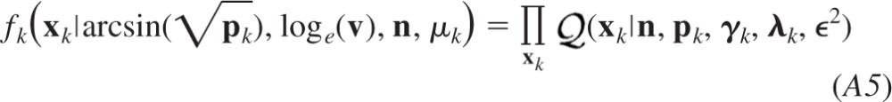Calculation of the log likelihood L_k, however, is computationally more efficient since this transforms the product to a summation.

The computation of the log likelihood is, however, not trivial. Although the prior probability matrix occupies three dimensions, the number of Bernoulli successes i represented in the quantal likelihood function constitutes a fourth dimension. Additionally, the data x_k and the different probability conditions associated with the means μ_k increases the dimensionality to six. Fortunately, only two of the parameters [i.e., arcsin($\sqrt{p_k}$) and log_e(v)] are continuous; empirically we find the analysis is sufficiently accurate at a resolution of 128 for both. The final calculation of each posterior f_k[arcsin($\sqrt{p_k}$), log_e(v), n|x_k, μ_k] can be obtained from the corresponding log likelihood L_k by normalization of its exponential to unity.

Probabilistic information that facilitates estimation of the quantal parameters contained in the different posteriors f_k[arcsin($\sqrt{p_k}$), log_e(v), n|x_k, μ_k], however, remains separated according to the partitions in the data for different values of k. The distributions of each set of observations x_k will differ from one another as a result of differences in the release probabilities p_k reflected in the respective means μ_k. Our first conditioned term arcsin($\sqrt{p_k}$) would thus be explicitly dependent on the mean response μ_k, whereas this would not be the case for the remaining parameters log_e(v) and n.

Inferential information can only by combined using product rule if the individual components are independent and identically distributed according to common parameters. The functional relationship between the parameter derived from the release probability arcsin ($\sqrt{p_k}$) and each mean μ_k precludes direct multiplication of the probabilities among f_k(arcsin($\sqrt{p_k}$), log_e(v), n|x_k, μ_k) since the values of p_k differ and would therefore not be identically distributed across k. First we must exclude any explicit dependence of each posterior on the release probability p_k.

For efficient combination of the information from different conditions of probability, we consider the ideal parameters ψ that are explicitly independent of release probability yet are associated with the optimal family of conditional posterior probabilities f_k(ψ|x_k, μ_k). Intuitively, the amplitude distribution of responses observed at low release probabilities most readily yields the quantal size q. At high probabilities, however, the data best facilitates estimation of the maximal response r, which we define as the mean response μ when the probability of release p is one, or: r = nq.

Division of the maximal response r by the quantal size q can thus be used to represent the number of release sites n. We also wish to estimate the gamma shaping parameter γ since this defines the shape of the underlying quantal distribution. Our ideal parameters ψ = (q, γ, r) can be expressed with respect to our present parameters (arcsin($\sqrt{p_k}$), log_e(v), n) using invertible functions, and we can thus conditionally marginalize f_k(arcsin($\sqrt{p_k}$), log_e(v), n|x_k, μ_k) to express a new family of conditional posteriors f_k(q, γ, r|x_k, μ_k) using Eq. 24. Since our implementation is discrete, we perform the conditional marginalization by summation over the three-dimensional space as defined by our new parameters.

$$f_k\left(\text{q},\gamma ,\text{r}|{\text{x}}_k,{\mu }_k\right)={\displaystyle \sum _{\frac{{\mu }_k}{{\text{np}}_k}=q}{\displaystyle \sum _{\frac{1}{{\text{v}}^2}}{\displaystyle \sum _{\frac{{\mu }_k}{{\text{P}}_k}=r}{f}_k\left(\arcsin \left(\sqrt{{\text{p}}_k}\right),{\log }_e\left(\text{v}\right),\hspace{0.17em}\text{n}|{\text{x}}_{\text{k}},{\mu }_k\right)}}}$$ (A7)

All of the new parameters (q, γ, r) are independent of the release probability p_k and are thus not subscripted. Since values for the gamma shaping parameter γ are already uniquely determined by only the logarithm of coefficient of variation log_e(ν), its conditional marginalization shown in Eq. 34 is computationally optimal if their respective values are intermapped directly. The quantal size q and maximal response r parameters are most efficiently sampled logarithmically since the upper limits may be several orders of magnitude greater than their respective lower limits. Since neither term is discrete, they are sampled continuously; again we find empirically a resolution of 128 sufficiently accurate.

Our intention is to obtain a single posterior f_k(q, γ, r|X) that constitutes the probability distribution of the parameters (q, γ, r) given the data X. The advantage of a probabilistic approach is that this is readily accomplished using simple laws of probability. Since all parameters (q, γ, r) are independent of the release probability p_k we assume independent conditioning effects of x_k and μ_k on each of the posteriors. Consequently, the family of posteriors f_k(q, γ, r|x_k, μ_k) must constitute mutually independent representations of a common underlying probability distribution. We thus use product rule to calculate a joint posterior distribution for the parameters (q, γ, r) that is conditioned by all conditions of release probability represented for the entire set data X by the first moments .

Neither the data nor first moments are represented as vectors on the left hand side because here each constitute a single concept. We also drop the subscript variable k since the three dimensional probability matrix is not conditioned solely by any single condition of release probability p_k. The joint posterior f(q, γ, r, |) is expressed using chain rule

Since the term denotes a single entity that represents the means which are fully determined by the data , the probabilities f(q, γ, r, |) and f(q, γ, r|)equate. The multiple f(|) is therefore a scalar that serves only as a trivial constant. Our intention of obtaining the posterior distribution f(q, γ, r|) is thus achieved by normalization of the result of the product expressed Eq. 35.

The marginal posterior probabilities for each of the quantal parameters f(q|), f(γ|), and f(r|) are obtained by summation of the joint posterior f(q, γ, r|) in the dimensions that marginalize the other two terms. Maximum a posteriori, moment-, or median-based measures provide estimates for the quantal size q̂, gamma shaping parameter γ̂, and the maximal response r̂. The cumulative distribution of each marginal posterior can be sampled to provide confidence limits for each of the quantal parameters. Probabilities of release for each condition is estimated by dividing the associated mean of the evoked synaptic responses by the estimated maximal response r̂ whereas estimates for the number of release sites n̂, the gamma scaling parameter λ̂, and the coefficient of variation v̂ is calculated using the following functional relations:

$$\widehat{n}=\frac{\widehat{r}}{\widehat{q}},\widehat{\lambda }=\frac{\widehat{q}}{\widehat{\gamma }},\widehat{v}=\sqrt{\frac{1}{\widehat{\gamma }}}$$ (A11)

Modeling heterogeneous release probabilities.

Optical recordings of individual synapses in hippocampal cultures have shown heterogeneity in the probability of release across release sites (Murthy et al. 1997). This heterogeneity can be modeled using a beta probability density function because it can assume a wide variety of shapes that are representative of the distribution of release probabilities across different sites (Silver 2003). An additional dimension in the priors and likelihood terms in the BQA implementation described above can be included to model the release probabilities p across release sites using a beta probability density function (p|α, β), where α and β are the shaping parameters.

Increases in the value of α represents a greater homogeneity in the release probabilities p. The mean release probability p̄_k for the kth condition are modeled as described for the binomial case except including an additional dimension to model the homogeneity α independently. Since α is always positive, we assign a uniform probability density function for log(α) as the marginal prior, and calculate corresponding values for β_k according to their functional relation:

$${\beta }_k=\alpha \left(\frac{1-{\overline{p}}_k}{{\overline{p}}_k}\right)$$ (A13)

With a beta model, the probability distribution of observing i total successes from n release sites would no longer conform to the binomial mass function expressed in Eq. 1 due to the heterogeneity in release probabilities. To our knowledge, there is no analytical expression for the analogous probability mass function ′(i|n, p̄_k, α). Consequently we resorted to numerical methods described below.

The beta cumulative density function was sampled evenly to assign Bernoulli probabilities of release to each of n release sites according to a beta distribution of mean p̄_k and uniformity α. Probabilities of every permutation of success and failure of release were evaluated using the product rule to construct an n-dimensional joint probability mass function of size 2ⁿ. The sum rule was then used iteratively to accumulate the probabilities of observing i total successes from the joint probability mass function by conditional marginalization to calculate ′(i|n, p̄_k, α) for i = {0, 1, …, n}.

REFERENCES

- Beato M. The time course of transmitter at glycinergic synapses onto motoneurons. J Neurosci 28: 7412–7425, 2008 [DOI] [PMC free article] [PubMed] [Google Scholar]
- Bekkers J. Quantal analysis of synaptic transmission in the central nervous system. Curr Opin Neurobiol 4: 360–365, 1994 [DOI] [PubMed] [Google Scholar]
- Bekkers J, Clements J. Quantal amplitude and quantal variance of strontium-induced asynchronous epscs in rat dentate granule neurons. J Physiol 516: 227–248, 1999 [DOI] [PMC free article] [PubMed] [Google Scholar]
- Bekkers J, Richerson G, Stevens C. Origin of variability in quantal size in cultured hippocampal neurons and hippocampal slices. Proc Natl Acad Sci USA 87: 5359–5362, 1990 [DOI] [PMC free article] [PubMed] [Google Scholar]
- Bennett M, Florin T. A statistical analysis of the release of acetylcholine at newly formed synapses in striated muscle. J Physiol 238: 93–107, 1974 [DOI] [PMC free article] [PubMed] [Google Scholar]
- Bhumbra G, Dyball R. Reading between the spikes of the hypothalamic neural code. J Neuroendocrinol 22: 1239–1250, 2010 [DOI] [PubMed] [Google Scholar]
- Bhumbra GS, Dyball RE. Spike coding from the perspective of a neurone. Cogn Proc 6: 157–176, 2005 [DOI] [PubMed] [Google Scholar]
- Boyd I, Martin A. The end plate potential in mammalian muscle. J Physiol 132: 74–91, 1956 [DOI] [PMC free article] [PubMed] [Google Scholar]
- Brown T, Perkel D, Feldman M. Evoked neurotransmitter release: statistical effects of nonuniformity and nonstationarity. Proc Natl Acad Sci USA 73: 2913, 1976 [DOI] [PMC free article] [PubMed] [Google Scholar]
- Christensen B, Martin A. Estimates of probability of transmitter release at the mammalian neuromuscular junction. J Physiol 210: 933–945, 1970 [DOI] [PMC free article] [PubMed] [Google Scholar]
- Clements J. Variance-mean analysis: a simple and reliable approach for investigating synaptic transmission and modulation. J Neurosci Meth 130: 115–125, 2003 [DOI] [PubMed] [Google Scholar]
- Clements J, Silver R. Unveiling synaptic plasticity: a new graphical and analytical approach. Trends Neurosci 23: 105–113, 2000 [DOI] [PubMed] [Google Scholar]
- Del Castillo J, Engbaek L. The nature of the neuromuscular block produced by magnesium. J Physiol 124: 370–384, 1954 [DOI] [PMC free article] [PubMed] [Google Scholar]
- Del Castillo J, Katz B. Quantal components of the end plate potential. J Physiol 124: 560–573, 1954 [DOI] [PMC free article] [PubMed] [Google Scholar]
- Diana MA, Marty A. Characterization of depolarization-induced suppression of inhibition using paired interneuron-purkinje cell recordings. J Neurosci 23: 5906–5918, 2003 [DOI] [PMC free article] [PubMed] [Google Scholar]
- Edwards F, Konnerth A, Sakmann B. Quantal analysis of inhibitory synaptic transmission in the dentate gyrus of rat hippocampal slices: a patch-clamp study. J Physiol 430: 213–249, 1990 [DOI] [PMC free article] [PubMed] [Google Scholar]
- Faber D, Korn H. Unitary conductance changes at teleost mauthner cell 43 glycinergic synapses: a voltage-clamp and pharmacologic analysis. J Neurophysiol 60: 1982–1999, 1988 [DOI] [PubMed] [Google Scholar]
- Fatt P, Katz B. Spontaneous subthreshold activity at motor nerve endings. J Physiol: 109–128, 1952 [PMC free article] [PubMed] [Google Scholar]
- Fisher R. On the mathematical foundations of theoretical statistics. Philos Trans R Soc Lond A Math Phys Sci 222: 309–368, 1922 [DOI] [PMC free article] [PubMed] [Google Scholar]
- Fisher R. Two new properties of mathematical likelihood. Proc R Soc Lond A Math Phys Sci 144: 285–307, 1934 [Google Scholar]
- Forti L, Bossi M, Bergamaschi A, Villa A, Malgaroli A. Loosepatch recordings of single quanta at individual hippocampal synapses. Nature 388: 874–878, 1997 [DOI] [PubMed] [Google Scholar]
- Hanse E, Gustafsson B. Quantal variability at glutamatergic synapses in area ca1 of the rat neonatal hippocampus. J Physiol 531: 467–480, 2001 [DOI] [PMC free article] [PubMed] [Google Scholar]
- Huzurbazar V. The likelihood equation, consistency and the maxima of the likelihood function. Ann Eugen 14: 185, 1948 [DOI] [PubMed] [Google Scholar]
- Jaynes E. Probability Theory: the Logic of Science. Cambridge, UK: Cambridge Univ. Press, 2003 [Google Scholar]
- Jeffreys H. An invariant form for the prior probability in estimation problems. Proc R Soc Lond A Math Phys Sci 186: 453–461, 1946 [DOI] [PubMed] [Google Scholar]
- Jeffreys H. Theory of Probability. Oxford, UK: Oxford Univ Press, 1998 [Google Scholar]
- Katz B, Miledi R. A study of spontaneous miniature potentials in spinal motoneurones. J Physiol 168: 389, 1963 [DOI] [PMC free article] [PubMed] [Google Scholar]
- Korn H, Burnod Y, Faber D. Spontaneous quantal currents in a central neuron match predictions from binomial analysis of evoked responses. Proc Natl Acad Sci USA 84: 5981–5985, 1987 [DOI] [PMC free article] [PubMed] [Google Scholar]
- Korn H, Mallet A, Triller A, Faber D. Transmission at a central inhibitory synapse. II. Quantal description of release, with a physical correlate for binomial n. J Neurophysiol 48: 679–707, 1982 [DOI] [PubMed] [Google Scholar]
- Korn H, Triller A, Mallet A, Faber D. Fluctuating responses at a central synapse: n of binomial fit predicts number of stained presynaptic boutons. Science 213: 898–901, 1981 [DOI] [PubMed] [Google Scholar]
- Kullmann D. Quantal variability of excitatory transmission in the hippocampus: implications for the opening probability of fast glutamate-gated channels. Proceed Biol Sci 253: 107–116, 1993 [DOI] [PubMed] [Google Scholar]
- Kullmann D, Nicoll R. Long-term potentiation is associated with increases in quantal content and quantal amplitude. Nature 357: 240–244, 1992 [DOI] [PubMed] [Google Scholar]
- Kuno M. Quantal components of excitatory synaptic potentials in spinal motoneurones. J Physiol 175: 81–99, 1964 [DOI] [PMC free article] [PubMed] [Google Scholar]
- Kuno M. Quantum aspects of central and ganglionic synaptic transmission in vertebrates. Physiol Rev 51: 647–678, 1971 [DOI] [PubMed] [Google Scholar]
- Kuno M, Weakly J. Quantal components of the inhibitory synaptic potential in spinal motoneurones of the cat. J Physiol 224: 287–303, 1972 [DOI] [PMC free article] [PubMed] [Google Scholar]
- Liley A. The quantal components of the mammalian end plate potential. J Physiol 133: 571–587, 1956 [DOI] [PMC free article] [PubMed] [Google Scholar]
- Liu G, Feldman J. Quantal synaptic transmission in phrenic motor nucleus. J Neurophysiol 68: 1468–1471, 1992 [DOI] [PubMed] [Google Scholar]
- MacLachlan E. An analysis of the release of acetylcholine from preganglionic nerve terminals. J Physiol 245: 447–466, 1975 [DOI] [PMC free article] [PubMed] [Google Scholar]
- Miyamoto M. Binomial analysis of quantal transmitter release at glycerol treated frog neuromuscular junctions. J Physiol 250: 121–142, 1975 [DOI] [PMC free article] [PubMed] [Google Scholar]
- Murthy V, Sejnowski T, Stevens C. Heterogeneous release properties of visualized individual hippocampal synapses. Neuron 18: 599–612, 1997 [DOI] [PubMed] [Google Scholar]
- Peizer DB, Pratt JW. A normal approximation for binomial, F, beta, and other common, related tail probabilities, I. J Am Stat Assoc 63: 1416–1456, 1968 [Google Scholar]
- Redman S. Quantal analysis of synaptic potentials in neurons of the central nervous system. Physiol Rev 70: 165–198, 1990 [DOI] [PubMed] [Google Scholar]
- Robinson J. Estimation of parameters for a model of transmitter release at synapses. Biometrics 31: 61–68, 1976 [PubMed] [Google Scholar]
- Silver R. Estimation of nonuniform quantal parameters with multipleprobability fluctuation analysis: theory, application and limitations. J Neurosci Meth 130: 127–141, 2003 [DOI] [PubMed] [Google Scholar]
- Silver R, Cull-Candy S, Takahashi T. Non-nmda glutamate receptor occupancy and open probability at a rat cerebellar synapse with single and multiple release sites. J Physiol 494: 231–250, 1996 [DOI] [PMC free article] [PubMed] [Google Scholar]
- Silver R, Momiyama A, Cull-Candy S. Locus of frequency-dependent depression identified with multiple-probability fluctuation analysis at rat climbing fibre-purkinje cell synapses. J Physiol 510: 881–902, 1998 [DOI] [PMC free article] [PubMed] [Google Scholar]
- Stern P, Edwards F, Sakmann B. Fast and slow components of unitary epscs on stellate cells elicited by focal stimulation in slices of rat visual cortex. J Physiol 449: 247–278, 1992 [DOI] [PMC free article] [PubMed] [Google Scholar]
- Stricker C, Field A, Redman S. Statistical analysis of amplitude fluctuations in epscs evoked in rat ca1 pyramidal neurones in vitro. J Physiol 490: 419–441, 1996 [DOI] [PMC free article] [PubMed] [Google Scholar]
- Tong G, Jahr C. Multivesicular release from excitatory synapses of cultured hippocampal neurons. Neuron 12: 51–59, 1994 [DOI] [PubMed] [Google Scholar]
- Turner D, West M. Bayesian analysis of mixtures applied to postsynnaptic potential fluctuations. J. Neurosci Meth 47: 1–21, 1993 [DOI] [PubMed] [Google Scholar]
- Walmsley B. Interpretation of “quantal” peaks in distributions of evoked synaptic transmission at central synapses. Proc Biol Sci 261: 245–250, 1995 [DOI] [PubMed] [Google Scholar]