Constant electric field simulations of the membrane potential illustrated with simple systems

Abstract

Advances in modern computational methods and technology make it possible to carry out extensive molecular dynamics simulations of complex membrane proteins based on detailed atomic models. The ultimate goal of such detailed simulations is to produce trajectories in which the behavior of the system is as realistic as possible. A critical aspect that requires consideration in the case of biological membrane systems is the existence of a net electric potential difference across the membrane. For meaningful computations, it is important to have well validated methodologies for incorporating the latter in molecular dynamics simulations. A widely used treatment of the membrane potential in molecular dynamics consists of applying an external uniform electric field E perpendicular to the membrane. The field acts on all charged particles throughout the simulated system, and the resulting applied membrane potential V is equal to the applied electric field times the length of the periodic cell in the direction perpendicular to the membrane. A series of test simulations based on simple membrane-slab models are carried out to clarify the consequences of the applied field. These illustrative tests demonstrate that the constant-field method is a simple and valid approach for accounting for the membrane potential in molecular dynamics studies of biomolecular systems.

1. Introduction

The electric potential difference across biological membranes plays a central role in many essential biological processes [1]. In living cells, the distribution of ions on both sides of the membrane is actively maintained by ion pumps and transporters, and the membrane potential results from the ion concentration gradients and the relative permeation of the membrane by the various ionic species. In the laboratory, it is also possible to artificially impose a potential difference across a membrane through the use of ion-exchange electrodes, a technique widely used in electrophysiology. Nevertheless, whether one is attempting to realistically model cellular processes or electrophysiological experiments, the physical underpinning of the potential is identical in both cases: the bulk ionic solutions remain electrically neutral overall and the potential difference across the membrane arises from a very small charge imbalance distributed in the neighborhood of the membrane-solution interface. The membrane responds as a classical linear capacitor and the potential difference V arising from the net charge separation ΔQ is V = Q/C. In the case of phospholipid bilayers, a membrane potential of 100 mV corresponds to a ΔQ of one elementary charge for each 250 Å × 250 Å area of membrane. Thus, a sizable potential difference across the membrane is associated with an extremely small charge separation. Accounting for this potential difference in simulations requires a well defined conceptual framework.

A linearized Poisson-Boltzmann theory modified to account for the membrane potential was formulated on the basis of a continuum electrostatic representation to account for the membrane potential [2]. The PB-V theory provides a conceptually transparent, albeit approximate, description of the membrane potential and allows for the calculation of several quantities of interest, such as the voltage profile along channels and vestibules of complex irregular shapes [3, 4], and the gating charge of intrinsic membrane proteins [2, 5–8]. However, the PB-V theory does not directly provide a method to include the membrane potential in all-atom MD simulations with explicit solvent and membrane. Such MD simulations are normally carried out under periodic boundary conditions (PBC) to reduce finite-size effects. Thus, the bulk ionic solutions on both sides of a membrane in a PBC system are actually the same liquid phase, which poses several challenges when one tries to implement a potential difference and concentration gradients across the membrane. For this reason, realistically incorporating the effect of the membrane potential in all-atom MD requires careful consideration. Over the past decade a few different strategies have been developed to circumvent the issue of periodicity in all-atom MD simulations.

The most direct approach to simulating a membrane potential consists of constructing a system that comprises two parallel bilayer membranes with two separate bulk phases [9, 10]. Different ionic concentrations in each bath can be introduced to create a realistic transmembrane potential. The dual-membrane approach has been used to study the initial stages of ion channel gating over a 10-nanosecond time scale [11] as well as electroporation of the membrane by ions [12, 13]. However, this approach considerably increases the size of the simulated systems and the computational cost. Nonetheless, the dual-membrane method might become more popular as computational power increases and simulations of larger systems become accessible, ultimately leading to simulations of near complete liposome-like systems. A slightly less demanding alternative to the dual-bilayer method consists of replacing one of the two membranes by a vacuum slab that effectively acts as a physical barrier to separate and isolate the two bulk solutions on both sides of the membrane [14]. With this approach, a charge imbalance between the two sides of a single membrane may be introduced to produce a transmembrane voltage [15, 16]. The dual-membrane and vacuum slab methods realistically incorporate the transmembrane electric potential in biomolecular dynamics simulations. In both cases, the resulting transmembrane potential is not known a priori, as it depends on the specific physical characteristics of the simulated bilayer and the imbalance of charge that is introduced in the system. Of particular importance, the actual value of the applied transmembrane potential may vary considerably (by hundreds of millivolts) upon a single permeation event [14], or if an embedded membrane protein carrying charged residues changes its conformation. In practice, the actual potential difference V needs to be constantly monitored and the charge imbalance ΔQ adjusted to prevent large changes during simulations. This poses some challenges because of the large membrane capacitance. For example, the transfer of a single elementary charge for each membrane patch of area 500 Å × 500 Å is suffcient to shift the membrane potential by about 25 mV. Lastly, the imposition of a very small potential can become difficult, requiring the enlargement of the simulated system to increase the area of the membrane or the inclusion of dummy particles with a fraction of elementary charge.

A different approach to account for the membrane potential in MD simulations consists of introducing a uniform electric field E throughout the entire simulated periodic cell containing the membrane system [17–19]. This gives rise to a force q_i · E that applies to all charges q_i in the simulation. The electric field is directed perpendicular to the membrane plane and must have a magnitude E = V/L_z, where L_z is the length of the PBC simulation box in that direction. Thus, the value of the applied voltage V is known a priori and the magnitude of the applied field depends only on the size of the simulation box L_z, with no need for a dual bilayer or an enlarged system with a vacuum slab. The pioneering application of the constant electric field approach in Aksimentiev and Schulten (2005) [20] demonstrated its ability to quantitatively determine the conductance of a membrane channel from only its X-ray structure. This approach has also been successfully used in many other applications studying ion conduction [21–26], voltage-regulated water flux [27–29], insertion of peptides into membranes [30], electroporation [31–34], translocation of DNA, ions, and large biomolecules through nanopores [33, 35–40], and induced conformational changes of membrane proteins [41–43].

The theoretical foundation of the constant field method has been clarified previously: it represents the influence of two aqueous salt bath solutions held at different voltages via an electromotive force (EMF) on a subsystem of interest [44]. Nevertheless, the method retains a certain appearance of artificiality that may be cause for confusion and concern. For example, it is not immediately apparent that the actual potential V imposed across a membrane in MD simulation in which a constant uniform electric field E is applied is truly equal to E · Lz, regardless of the shape of the protein/membrane interface. Furthermore, the constant field method adds a constant force, q_iV/L_z, acting on all the charges in the system, regardless of their position. However, it is understood that the transmembrane potential arises from a microscopic charge separation and that the net average electric field in the aqueous region should be very small.

It is the goal of this brief review to address the aforementioned concerns and to clarify the application of the constant electric field method. To help illustrate the significance of the constant field method, we carried out a number of MD simulations based on simple model systems composed of a low-dielectric pseudo-membrane slab with different fixed geometries. It is shown that applying an external electric field is, indeed, a valid method for generating a potential difference across a membrane in MD simulations. We also examine potentially subtle issues of system size dependence, both in terms of how one calculates the potential from the applied field and in how that dependence is manifested in equilibrium and non-equilibrium properties of the system.

2. Results

2.1. Applied constant electric field in the context of periodic boundary conditions

The presence of a potential difference across a membrane unavoidably breaks periodicity. Nevertheless, the equivalence of the forces arising from the constant applied electric field across the boundary ensures that there is no discontinuity in the force acting on a given particle when crossing it. The net result of a particle crossing the periodic boundary is akin to passing through a virtual circuit with an embedded EMF, i.e., a battery [44]. This virtual EMF provides the work that gives rise to the bulk phase polarization (and slight charge imbalance if there are mobile ions) across the simulation cell, which causes the potential difference. To understand how the membrane potential difference relates to the periodic boundaries, it is helpful to observe how it is realized in various systems.

As visualized in Fig. 1, a constant applied electric field generates a linear potential across the entire unit cell. However, what matters is the total potential difference across the membrane, which is the predominant quantity underlying biologically relevant events and the quantity that one typically desires to control in a simulation. A uniform medium such as an aqueous salt solution will naturally self-organize to reduce as much as possible the magnitude of any net average electric field. This behavior is akin to good conductors that expel all electric fields from their interior. The rearrangement of the bulk medium to a non-uniform distribution generates its own reaction field that, when summed with the external field, gives the resulting, total field. Because the change in potential must take place somewhere within the system, it becomes naturally concentrated at an immobile insulating membrane, regardless of its shape or size, with a characteristic decay away from it. Despite the non-periodicity of the total potential, the force experienced by a charged atom across the periodic boundary (computed from the first derivative of the total potential) is continuous.

Figure 1.

Schematic description of the constant electric field methodology. In the periodic system, the applied constant field is associated with a linear potential, which is combined with the reaction potential from the electrostatic interactions treated via particle mesh Ewald (PME) to generate the resulting total potential. Even though the total electrostatic potential is non-periodic, the reaction potential computed during the simulation (PME), as well as the forces (slopes of curves) from both the applied and total potential are compatible with periodic boundary conditions.

To demonstrate concretely the conceptual arguments made above, we begin with the simplest system, a uniform hydrophobic slab 20-Å thick in the center of an aqueous NaCl salt solution extending approximately 27 Å above and below (see Fig. 2A). The electric field, constant in the z direction and zero in the x and y directions, is determined from the desired potential difference, V = 500 mV here, across the entire unit cell through the equation E_z = V/L_z. In this equation, L_z refers to the size of the entire periodic cell, including membrane and water (~75 Å). The resulting potential for the entire system, averaged over a 10-ns simulation and shown in Fig. 2B, is clearly focused to the region of the slab, despite the constant external field applied. Thus, the entire 500-mV potential drop occurs across the membrane only, with the potential difference in the bulk regions above and below being zero.

Figure 2.

Membrane slab systems. (A) Full simulation system for the simple membrane slab shown as space-filling spheres with the membrane colored in blue; the water in red and white; and Na⁺ and Cl⁻ ions in yellow and cyan, respectively. (B) Time-averaged electrostatic potential for the system in (A). The color gradient to the right indicates the scale for the potential in units of Volts. (C,D) Simulation system and potential identical to those in (A,B) except with the system length doubled and the applied field halved. (E) Potential along the z-axis for the system in A (black) and in C (red).

2.2. System size and resulting membrane potential

How should the applied field be treated if the system size is doubled while the thickness of the membrane is kept constant as illustrated in Fig. 2C? According to the relation E_z = V/L_z, if L_z is doubled, then the external applied field E_z ought to be divided by two in order to maintain the same value of V. Again, this concept is illustrated by considering the simple membrane slab under a reduced applied field. As explicitly demonstrated by the simulation, the resulting average potential throughout the system is identical to that for the smaller system (compare Fig. 2D to Fig. 2B and the curves in Fig. 2E). As before, the expected potential difference of 500 mV is focused to the region of the membrane only.

To further illustrate that the applied field necessary to enforce a given voltage depends only on the size of the simulation box and is independent of the shape of the membrane, we consider the same hydrophobic slab but with a central part cut out. This cutout reaches halfway into the membrane, sloping inward to the thinner part of the membrane (see Fig. 3A). The resulting trapezoidal-cutout slab was simulated under the same conditions as the uniform slab, namely two system sizes and an expected potential difference of 500 mV across the entire unit cell. As before, the resulting time-averaged potential throughout the system is identical for the two system sizes provided that the applied E_z is halved for the larger system (see Figs. 3B,C). In particular, the full potential difference V is typically focused to the insulating membrane alone, despite its variations in thickness.

Figure 3.

Alternative simulated membrane geometries. (A) Simulation system for the membrane with a trapezoidal cutout, colored as in Fig. 2A. (B,C) Time-averaged potential for the system in (A) and the same system with its length in z doubled, respectively. (D) Potential along z, centered in x and y, taken from those in B (black) and C (red). (E–H) System and potentials shown as in (A–D) for the membrane with a rectangular cutout.

Taking the reduction in membrane thickness to its extreme limit, a membrane was prepared in which a central box-shaped region is removed such that only a single layer of hydrophobic atoms separates the two bulk regions (see Figs. 3E–H). Although the applied field is uniform, in both the smaller and larger systems the resulting electrostatic potentials are identical, with the potential difference being focused to the fixed membrane only. This focusing tightly couples the potential difference to the membrane shape, and can thus generate large electric fields in the thinnest regions, such as the single fixed layer in the system in Fig. 3E. All these examples demonstrate that the resulting potential difference in any system depends only on the applied field and the size of the simulation unit cell, not on the particular membrane size or geometry. The microscopic details of the shape and size of the molecule system are irrelevant and do not determine the potential difference imposed by the constant field method.

2.3. Non-equilibrium dissipative finite-size effects

The results displayed in Figs. 2 and 3 show that the average membrane potential profile across the system is not very sensitive to the size of the simulated system (as long as E is given by V/L_z). Another finite-size effect, though not specifically relevant to the situation considered here with an applied external electric field, is associated with the system's periodicity and the planar membrane geometry [45, 46]. It arises from the difference in self-interaction between the ion and its periodic images when the ion is located in the low-dielectric membrane region (or inside a channel), where its field is not as effciently shielded compared to when the ion is located in the high-dielectric bulk solution [45, 46]. The magnitude of such a spurious self-interaction in periodic systems can be estimated, for example, by using a continuum electrostatics approximation [45–47]. However, based on the size of the systems simulated here (at least 44 Å between images), the correction is expected to be negligible [48].

Such relative lack of sensitivity of the results on the size of the simulated system size must, however be considered with caution. The robustness of average equilibrium properties is largely predetermined by the gross structural features of the systems, in qualitative accord with continuum electrostatics. Once the system reaches thermodynamic equilibrium, the spatial distribution and orientation of the water molecules and mobile ions is rearranged to essentially cancel out the applied external field in the bulk phase regions and, as a result, the potential drop occurs mainly across the non-conducting low-dielectric insulating regions. However, non-equilibrium properties, such as ion fluxes through membranes or the rate of conformational transitions, might be more sensitive to the size of the system.

To illustrate the possibility of size-dependent effects on transport phenomena, we examine the rate of ion permeation through a membrane slab with a generic pore in two systems of different sizes. To simulate ion conduction, a 20-Å-diameter cylindrical pore was cut through the fixed membrane slab and the resulting system was subjected to an external electric field of 500 mV in one set of simulations and 1 V in another set (see Figs. 4A–C). In one system the length of the bulk salt solution is larger such that the simulation box is twice as long in the z direction compared to the other, with L_z = 154 Å and L_z = 74 Å, respectively. In all other aspects, the membrane slab and pore are identical. Any atomic charge movement in the microscopic system is associated with a detectable current going through the virtual EMF circuit [44]. It follows, then, that the steady-state ionic flux through this model pore under an applied voltage can be calculated from the total displacement current [20],

$$I\left(t\right)=\frac{1}{L_z}\sum _{\text{all atoms}}{q}_i{\stackrel{.}{z}}_i\left(t\right),$$ (1)

where ${\stackrel{.}{z}}_i\left(t\right)$ is the velocity of particle i carrying in the z-direction. Alternatively, it is possible to consider the integrated form of Eq. (1),

$$Q\left(t\right)=\frac{1}{L_z}\sum _{\text{all atoms}}{q}_i\left[z_i\right(t)-z_i(0\left)\right],$$ (2)

where z_i(t) represent the continuous “unwrapped” coordinates of the atoms, i.e., not folded back into the periodic box. The average current I(t) can then be evaluated as the limiting value of Q(t)/t as t → ∞ [44]. We note that because of the fixed membrane, there is no net drift of the system, which otherwise might need to be removed [20].

Figure 4.

Membrane with a 20-Å-diameter pore. (A) Simulation system. (B,C) Potentials for the smaller (B) and larger (C) pore-containing systems. (D) Potential along z as in Figs. 2E and 3D,H. (E,F) Current as a function of time for the smaller (E) and larger (F) systems. The inset of each graph shows the displacement charge Q over time.

At V = 500 mV, the current I_avg. = −3.06 ± 0.11 e/ns for the smaller system (74 Å long) while I_avg. = −2.91 ± 0.04 e/ns for the larger system (154 Å long). The current in each of the two systems was estimated from Eq. (2) by averaging the value of Q(t)/t over the final 2 ns of simulation. Although the currents are close, there is a small apparent difference. As a further test of potential size-dependent effects, the voltage difference was increased to 1 V. The results are shown in Figs. 4E, F for the two systems. The currents at 1 V are −6.13 ± 0.16 e/ns and −4.69 ± 0.08 e/ns for the smaller and larger systems, respectively. Here, the difference is clearly more important, showing that there is a size dependence of the current in these systems. Based on these currents, the total resistance extracted from the MD simulations at 500 mV is 1.02 ± 0.04 × 10⁹ Ω for the smaller system, and 1.07 ± 0.01 × 10⁹ Ω for the larger system, yielding an increase of 0.05 × 10⁹ Ω in the total resistance (~5%). The increase in total resistance extracted at 1 V is 0.31 × 10⁹ Ω, which is even larger (~26 %).

One may try to rationalize the observed size-dependence of the simulated ionic currents on the basis of simple macroscopic arguments. Assuming that the bulk solutions and the pore act as resistors connected in series, the total resistance is expressed according to Ohms' law as R_tot = R_pore + R_bulk [49]. If the resistance associated with the pore R_pore remains the same in both systems, then the increase in the total resistance should be explained by the increase in resistance in the bulk region. It is tempting to estimate the latter using the simple macroscopic approximation, R_bulk = ρL/A, where L and A are the length and the cross-sectional area of the bulk, respectively, and ρ is the bulk resistivity of the solution. However, this simple macroscopic expression assumes all ions flow to the pore along lines parallel to z, ignoring the complexities introduced by the membrane, bulk, and pore geometries. For instance, in the limit of a thermodynamically large system, an explicit dependence of the resistance on the system's length, L, persists, which would be inconsistent with single channel experiments [1]. The more relevant form of R_bulk that should be considered is known as the “access resistance” [1, 50–52],

$$R_{\text{access}}\approx 2{\int }_a^l\mathrm{d}r\frac{\rho }{2\pi r^2}=\frac{\rho (l-a)}{\pi al},$$ (3)

where a is the pore radius (10 Å) and l is the distance from the pore to the box edge, i.e., l = L/2; as l → ∞, R_access converges properly to a finite value. The resistivity of a 300 mM NaCl solution for the current force field is about 19.1 Ω·cm [53]. The length of the bulk region is 54 Å A and 134 Å for the smaller and larger systems, respectively. Using these values, the access resistance is estimated to be 0.038 × 10⁹ Ω for the smaller system, and 0.052 × 10⁹ Ω for the larger system, which yields an increase of about 0.014 × 10⁹. This value is considerably smaller than the changes of 0.05 × 10⁹ Ω at 500 mV and 0.31 × 10⁹ Ω at 1 V observed in the simulations, indicating that such a macroscopic argument does not explain the change in the observed resistance in the system fully. Changes in R_access can also be estimated from the voltage drop outside the pore (see Fig. 4D for the 1-V case). At 500 mV, R_access increases by a factor of 1.3 when comparing the larger to the smaller system, but only 1.12 at 1 V. For comparison, R_pore is 1.08 times greater at 500 mV and 1.12 times at 1 V, although it should be independent of system size and applied potential. That it is not suggests the presence of an additional size-dependent effect that is also sensitive to the strength of the field, which is greatest inside the pore.

These considerations suggest that the size-dependency of the ionic current in the simulations must arise from more subtle factors. This is best explained in the context of the effective dynamics of the permeating ions based on the Generalized Langevin equation [54]. Within such reduced dynamics, the basic ingredients controlling the rate of ion permeation are the potential of mean force (PMF), the membrane potential, and the effective friction. The latter is related to the rapidly fluctuating excess force, δF(t) = F(t) − 〈F〉, acting on a permeating ion inside the pore according to the fluctuation-dissipation theorem [55],

$$\gamma =\frac{1}{k_{B}T}{\int }_0^{\infty }\mathrm{d}tM\left(t\right)$$ (4)

where M(t) = 〈δF(t)δF(0)〉 is the memory function.

To quantify these effects, we calculated 〈F_tot〉, M(t), and γ for a chloride ion inside the pore under a potential difference of 1 V. Both the PMF and the membrane potential are equilibrium properties, and we have shown above that the latter is insensitive to the size of the simulated system. For the sake of completeness, the PMF for the ion in the absence of an applied field was also computed. The PMF, shown in Fig. 5, is largely flat at the pore's center, confirming that there is no systematic size-dependence of the mean force. In other words, 〈F〉 should be essentially equal in both the larger and smaller systems. Indeed, this was found to be the case: F_tot = 0.595 kcal/mol·Å for the larger system and F_tot = 0.562 kcal/mol·Å for the smaller one. However, it is expected that the memory function M(t) will display some size dependence because a larger fraction of the total force F(t) in the case of the smaller system is a constant component, qE_z, from the applied external field. Conversely, the fluctuating component of the force, which contributes directly to the effective friction via Eq. (4), makes up a larger fraction of the total force F(t) in the case of the larger system. In the larger system, the force due to the external field, qE = 0.150 kcal/mol·Å, is 27% of the total force, whereas in the smaller system, qE = 0.312 kcal/mol·Å is more than half of the total mean force. As a result, the effective friction is expected to be larger in the larger system, a size-dependent effect that should be apparent in the simulations. Shown in Fig. 6A, the force autocorrelation function rapidly decays toward zero within a few hundred femtoseconds (fs) for both systems. The friction coefficient γ, however, diverges within 3 ps in the two systems, with the ion in the smaller system experiencing a lower friction. As the time-independent force q · E_z approaches the total mean force 〈F〉, its quantitative impact on transport properties will become increasingly apparent.

Figure 5.

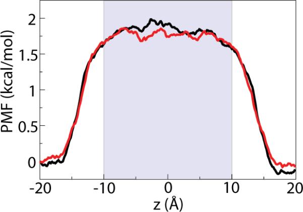
Potential of mean force (PMF) for a Cl⁻ ion in the 20-Å pore in the absence of an applied field. The black curve represents the system of size L and the red 2L; the extent of the pore is indicated by the shaded blue region. Implicit in the calculation of M(t) is the assumption that it does not depend on the position z of the ion [54]. The relatively flat PMF about z = 0 confirms that there is no contribution from a systematic mean force to the fluctuations.

Figure 6.

Effect of size on transport properties. In all panels, the black curve represents the system of length L and the red curve that of length 2L. (A) Memory function, M(t) for the chloride ion in the 20-Å pore. The inset is a close-up of the first 0.5 ps. (B) γ(t) for the two systems. (C,D) Memory function (C) and friction γ (D) for a simple charged particle with no Lennard-Jones interactions restrained in the center of a pure slab.

To further highlight the nature of the long-range effects that give rise to the size dependency, a simple charged particle with no Lennard-Jones interactions was restrained at the center of the membrane slab. The particle is only subject to long-range electrostatic interactions with the water molecules and the mobile ions in the bulk phase; there are no interactions with the uncharged particle forming the membrane slab. Both a large and a small system were simulated with an applied field corresponding to a membrane potential of 1 V. The calculated average forces are 1.01 and 0.993 kcal/mol·Å for the smaller and larger systems, respectively. As shown in Figs. 6C and D, the effective friction γ in the two systems is clearly different. In the larger system, there is a slowly decaying component to the force autocorrelation function, with an amplitude corresponding to a weak fluctuating force of 0.05 kcal/mol·Å decorrelating over a relaxation time of about 22 ps. To give some idea of the order of magnitude of such a contribution, a force of 0.05 kcal/mol·Å corresponds roughly to the force exerted by one TIP3 water molecule (dipole of 0.48862 eÅ) on an elementary charge at a distance of 15 Å, i.e., 332 · 0.48862/15³ = 0.05 kcal/mol·Å. In summary, a system that is too small may produce a proper transmembrane potential profile, yet allow artificially enhanced currents due to the reduced dissipative effects arising from long-range fluctuations.

3. Discussion

In light of the simulations with a constant field presented here, it is clear that the magnitude of the membrane potential is solely a function of the external field E and the length of the system L_z in the unit cell. The result is independent of the membrane thickness and of the shape of the low-dielectric material separating the bulk phases in the system. The resulting membrane voltage V is always equal to E · L_z. That the resulting V is indeed equal to E · L_z can be visualized directly by mapping the average electrostatic potential from the trajectories as shown in Figs. 2–4, and verified explicitly by calculating the free energy for charging a test particle at different locations in the system [42, 44].

Although V = E · L_z is a simple prescription, there remains quite some confusion regarding the relation between the applied field and the resulting membrane voltage in the literature. In a number of simulation studies aimed at incorporating the influence of a membrane potential via a constant electric field E, the actual reported value for the membrane potential V was calculated as E · Δ_z, where Δz was the thickness of the membrane in the system [26, 56]. Intuitively, this seems to be a reasonable choice because the average electric field is expected to be negligible throughout the high dielectric aqueous phases, and most of the voltage drop from the membrane potential occurs across the non-aqueous insulating regions in the system. However, one must exercise caution in invoking arguments based on a macroscopic representation because the correspondence to all-atom MD simulations with explicit solvent is not as straightforward as it may seem. While it is true that the resulting average membrane potential will mainly drop across the insulating region (the membrane), it is actually incorrect to ascribe the value of V as being equal to E_z times the effective thickness of this region when a constant external electric field is applied to all the charged atoms in an MD simulation. The confusion appears fairly widespread, although only a few publications provide the necessary information to know what was actually done (the value of the applied constant field, the length of the periodic simulation cell, and the membrane voltage must all be reported). A first example is a simulation study of the Shaker channel [56]. An external field of 4 mV/Å was applied, intended to represent a membrane potential of −100 mV, a value which was determined by dividing 100 mV by an assumed membrane thickness of 25 Å. However, the length of the periodic simulation cell in the z direction was 100 Å, which implies that the actual membrane potential applied during the simulation was underestimated by a factor of four. A second example is a simulation study of K⁺ conduction through the pore domain of the Kv1.2 channel [26]. The average ionic current was simulated for several different values of applied electric field to produce the I–V curve of the channel. The membrane voltage V reported in the study was calculated as E · Δz, where Δz was taken to be equal to the length of the selectivity filter of the channel (taken as the distance of 13.4 Å between Thr374 and Tyr377) [26]. The membrane potential that was actually applied in those simulations is E multiplied by the length L_z of the periodic simulation cell, ~85 Å. Thus, the reported voltage associated with the simulated currents in the I–V curves was underestimated by a factor of about six (~ 85/13.4 = 6.34). We do not dwell on these details as a matter of criticism of these previous studies, but to shed as much light as possible on the most common sources of confusion concerning the relationship between the applied electric field and the resulting membrane potential in MD simulations.

The constant electric field methodology provides an unambiguous and simple means to apply a voltage bias in membrane simulations. In contrast to the two alternative methodologies, namely the dual membrane and its extension with a vacuum slab, the constant field method allows simulations of ionic currents through biological channels at a constant membrane potential. The method has been implemented in several biomolecular simulation programs, which makes it readily available for membrane simulations. Using simple membrane slab systems, we have shown that the application of a constant electric field normal to the plane of the membrane produces a proper description of the membrane potential. In all cases, the resulting voltage is independent of the system being simulated and solely depends on E · L_z. However, non-equilibrium properties are more sensitive to the finite system size due to changes in the resistance and long-range dissipative effects. In part owing to its simplicity, the method has been applied in several simulation studies of membrane systems, including ion permeation in proteins and nanopores [20–26], electroporation [31–34], translocation of molecules through nanopores [33, 35–40], and conformational transitions in biological systems [41–43].

Appendix A. Model systems and simulation methodologies

The model membranes used throughout are constructed of individual carbon atoms arranged in a body-centered cubic lattice with a spacing of 4 Å. All membranes have six vertical layers at their maximum and, thus, a thickness of 20 Å, not accounting for the radius of the atoms themselves. In each simulated system the membrane is fully solvated above and below and ionized with Na⁺ and Cl⁻ ions at a concentration of 300 mM. System sizes for the membrane slab and for the slab with a 20-Å pore were 44 Å × 44 Å in the membrane plane and approximately 75 Å and 150 Å perpendicular to the membrane for systems of length L and 2L, respectively. For the slabs with a trapezoidal or square cutout, sizes were 68 Å × 68 Å × 75–150 Å. Atom counts for the systems range from 11,000 to 70,000 atoms. To prevent de-wetting of the interior of the cutout, a potential issue for hydrophobic surfaces [57], the oxygen atoms of one layer of water molecules were lightly (k = 0.5 kcal/mol Å·²) restrained along its surface. In the case of the 20-Å pore, restraints were reduced to k = 0.1 kcal/mol·Å² to minimize possible e ects on the current.

All simulations were run using NAMD 2.7 [58] and the CHARMM force field [59]. Periodic dimensions were kept fixed, and a constant temperature of 300 K was maintained using a Langevin thermostat with damping coefficient of 1 ps⁻¹, i.e., the NVT ensemble. A time step of 1 fs was used. Short-range non-bonded interactions were evaluated every other time step and were truncated at 12 Å with a switching function applied beginning at 10 Å. Long-range electrostatics were evaluated every fourth time step using the particle-mesh Ewald method.

Electrostatic potential maps were calculated using VMD′s PMEPot plugin [20, 60] along with Matlab. The potentials of mean force given in Fig. 5 were determined using the adaptive biasing force method as implemented in NAMD [58, 61, 62]. Images were prepared using VMD [60].

To compute the force autocorrelation function, the ion was harmonically restrained to z = 0 at the center of the 20-Å pore (force constant k = 10 kcal/mol·Å²) and the total fluctuating molecular force was taken to be that after subtracting the artificial restraint force [63]. In Eq. (4) the force F (t) should be calculated from a fixed particle; the restraint method used here yields equivalent results [64].

References

- [1].Hille B. Ion channels of excitable membranes. 3rd Edition Sinauer Associates; Sunderland, MA: 2001. [Google Scholar]
- [2].Roux B. The influence of the membrane potential on the free energy of an intrinsic protein. Biophys. J. 1997;73:2980–2989. doi: 10.1016/S0006-3495(97)78327-9. [DOI] [PMC free article] [PubMed] [Google Scholar]
- [3].Roux B, Bernèche S, Im W. Ion channels, permeation and electrostatics: Insight into the function of KcsA. Biochemistry. 2000;39:13295–13306. doi: 10.1021/bi001567v. [DOI] [PubMed] [Google Scholar]
- [4].Jogini V, Roux B. Electrostatics of the intracellular vestibule of K+ channels. J. Mol. Biol. 2005;354:272–288. doi: 10.1016/j.jmb.2005.09.031. [DOI] [PubMed] [Google Scholar]
- [5].Grabe MM, Lecar HH, Jan YN, Jan LY. A quantitative assessment of models for voltage-dependent gating of ion channels. Proc. Natl. Acad. Sci. USA. 2004;101:17640–17645. doi: 10.1073/pnas.0408116101. [DOI] [PMC free article] [PubMed] [Google Scholar]
- [6].Chanda B, Asamoah OK, Blunck R, Roux B, Bezanilla F. Gating charge displacement in voltage-gated ion channels involves limited transmembrane movement. Nature. 2005;436:852–856. doi: 10.1038/nature03888. [DOI] [PubMed] [Google Scholar]
- [7].Jogini V, Roux B. Dynamics of the Kv1.2 voltage-gated K+ channel in a membrane environment. Biophys. J. 2007;93:3070–3082. doi: 10.1529/biophysj.107.112540. [DOI] [PMC free article] [PubMed] [Google Scholar]
- [8].Pathak MM, Yarov-Yarovoy V, Agarwal G, Roux B, Barth P, Kohout S, Tombola F, Isacoff EY. Closing in on the resting state of the Shaker K(+) channel. Neuron. 2007;56:124–140. doi: 10.1016/j.neuron.2007.09.023. [DOI] [PubMed] [Google Scholar]
- [9].Sachs JN, Crozier PS, Woolf TB. Atomistic simulations of biologically realistic transmembrane potential gradients. J. Chem. Phys. 2004;121:10847–10851. doi: 10.1063/1.1826056. [DOI] [PubMed] [Google Scholar]
- [10].Gurtovenko AA, Vattulainen I. Pore formation coupled to ion transport through lipid membranes as induced by transmembrane ionic charge imbalance: Atomistic molecular dynamics study. J. Am. Chem. Soc. 2005;127:17570–17571. doi: 10.1021/ja053129n. [DOI] [PubMed] [Google Scholar]
- [11].Denning EJ, Crozier PS, Sachs JN, Woolf TB. From the gating charge response to pore domain movement: initial motion of Kv1.2 dynamics under physiological voltage changes. Mol. Membr. Biol. 2009;26:397–421. doi: 10.3109/09687680903278539. [DOI] [PMC free article] [PubMed] [Google Scholar]
- [12].Kandasamy SK, Larson RG. Cation and anion transport through hydrophilic pores in the lipid bilayers. J. Chem. Phys. 2006;125:074901. doi: 10.1063/1.2217737. [DOI] [PubMed] [Google Scholar]
- [13].Gurtovenko AA, Vattulainen I. Ion leakage through transient water pores in protein-free lipid membranes driven by transmembrane ionic charge imbalance. Biophys. J. 2007;92:1878–1890. doi: 10.1529/biophysj.106.094797. [DOI] [PMC free article] [PubMed] [Google Scholar]
- [14].Delemotte L, Dehez F, Treptow W, Tarek M. Modeling membranes under a transmembrane potential. J. Phys. Chem. B. 2008;112:5547–5550. doi: 10.1021/jp710846y. [DOI] [PubMed] [Google Scholar]
- [15].Treptow W, Tarek M, Klein ML. Initial response of the potassium channel voltage sensor to a transmembrane potential. J. Am. Chem. Soc. 2009;131:2107–2109. doi: 10.1021/ja807330g. [DOI] [PMC free article] [PubMed] [Google Scholar]
- [16].Delemotte L, Tarek M, Klein ML, Treptow W. Intermediate states of the Kv1.2 voltage sensor from atomistic molecular dynamics simulations. Proc. Natl. Acad. Sci. USA. 2011;127:6109–6114. doi: 10.1073/pnas.1102724108. [DOI] [PMC free article] [PubMed] [Google Scholar]
- [17].Suenaga A, Komeiji Y, Uebayasi M, Meguro T, Saito M, Yamato I. Computational observation of an ion permeation through a channel protein. Biosci. Rep. 1998;18:39–48. doi: 10.1023/a:1022292801256. [DOI] [PubMed] [Google Scholar]
- [18].Zhong QF, Husslein T, Moore PB, Newns DM, Pattnaik P, Klein ML. The M2 channel of influenza A virus - A molecular dynamics study. FEBS Lett. 1998;434:265–271. doi: 10.1016/s0014-5793(98)00988-0. [DOI] [PubMed] [Google Scholar]
- [19].Crozier PS, Henderson D, Rowley RL, Busath DD. Model channel ion currents in NaCl-extended simple point charge water solution with appliedfield molecular dynamics. Biophys. J. 2001;81:3077–3089. doi: 10.1016/S0006-3495(01)75946-2. [DOI] [PMC free article] [PubMed] [Google Scholar]
- [20].Aksimentiev A, Schulten K. Imaging alpha-hemolysin with molecular dynamics: Ionic conductance, osmotic permeability, and the electrostatic potential map. Biophys. J. 2005;88:3745–3761. doi: 10.1529/biophysj.104.058727. [DOI] [PMC free article] [PubMed] [Google Scholar]
- [21].Khalili-Araghi F, Tajkhorshid E, Schulten K. Dynamics of K+ ion conduction through Kv1.2. Biophys. J. 2006;91:L72–L74. doi: 10.1529/biophysj.106.091926. [DOI] [PMC free article] [PubMed] [Google Scholar]
- [22].Sotomayor M, Vasquez V, Perozo E, Schulten K. Ion conduction through MscS as determined by electrophysiology and simulation. Biophys. J. 2007;92:886–902. doi: 10.1529/biophysj.106.095232. [DOI] [PMC free article] [PubMed] [Google Scholar]
- [23].Siu SW, Böckmann RA. Electric field effects on membranes: gramicidin A as a test ground. J. Struct. Biol. 2007;157:545–556. doi: 10.1016/j.jsb.2006.10.005. [DOI] [PubMed] [Google Scholar]
- [24].Pezeshki S, Chimerel C, Bessonov AN, Winterhalter M, Kleinerkathöfer U. Understanding ion conductance on a molecular level: an all-atom modeling of the bacterial porin OmpF. Biophys. J. 2009;97:1898–1906. doi: 10.1016/j.bpj.2009.07.018. [DOI] [PMC free article] [PubMed] [Google Scholar]
- [25].Maffeo C, Aksimentiev A. Structure, dynamics, and ion conductance properties of the phospholamban pentamer. Biophys. J. 2009;96:4853–4865. doi: 10.1016/j.bpj.2009.03.053. [DOI] [PMC free article] [PubMed] [Google Scholar]
- [26].Jensen MØ, Borhani DW, Lindorff-Larsen K, Maragakis P, Jogini V, Eastwood MP, Dror RO, Shaw DE. Principles of conduction and hydrophobic gating in K+ channels. Proc. Natl. Acad. Sci. USA. 2010;107:5833–5838. doi: 10.1073/pnas.0911691107. [DOI] [PMC free article] [PubMed] [Google Scholar]
- [27].Hub JS, Aponte-Santamarfa C, Grubmüller H, de Groot BL. Voltage-regulated water flux through aquaporin channels in silico. Biophys. J. 2010;99:L97–L99. doi: 10.1016/j.bpj.2010.11.003. [DOI] [PMC free article] [PubMed] [Google Scholar]
- [28].Su J, Guo H. Control of unidirectional transport of single-file water molecules through carbon nanotubes in an electric field. ACS Nano. 2011;25:351–359. doi: 10.1021/nn1014616. [DOI] [PubMed] [Google Scholar]
- [29].Garate JA, English NJ, MacElroy JM. Static and alternating electric field and distance-dependent effects on carbon nanotube-assisted water self-diusion across lipid membranes. J. Chem. Phys. 2009;14:114508. doi: 10.1063/1.3227042. [DOI] [PubMed] [Google Scholar]
- [30].Tieleman DP, Berendsen HJ, Sansom MS. Voltage-dependent insertion of alamethicin at phospholipid/water and octane/water interfaces. Biophys. J. 2001;80:331–346. doi: 10.1016/S0006-3495(01)76018-3. [DOI] [PMC free article] [PubMed] [Google Scholar]
- [31].Tarek M. Membrane electroporation: a molecular dynamics simulation. Biophys. J. 2005;88:4045–4053. doi: 10.1529/biophysj.104.050617. [DOI] [PMC free article] [PubMed] [Google Scholar]
- [32].Böckmann R, de Groot BL, Kakorin S, Neumann E, Grubmüller H. Kinetics, statistics and energetics of lipid membrane electroporation studied by molecular dynamics simulations. Biophys. J. 2008;95:1837–1850. doi: 10.1529/biophysj.108.129437. [DOI] [PMC free article] [PubMed] [Google Scholar]
- [33].Vernier PT, Sun MJZY, Gundersen MA, Tieleman DP. Nanopore-facilitated, voltage-driven phosphatidylserine translocation in lipid bilayers-in cells and in silico. Phys. Biol. 2006;2:233–247. doi: 10.1088/1478-3975/3/4/001. [DOI] [PubMed] [Google Scholar]
- [34].Bockmann RA, de Groot BL, Kakorin S, Neumann E, Grubmuller H. Kinetics, statistics, and energetics of lipid membrane electroporation studied by molecular dynamics simulations. Biophys. J. 2008;95:1837–1850. doi: 10.1529/biophysj.108.129437. [DOI] [PMC free article] [PubMed] [Google Scholar]
- [35].Aksimentiev A, Heng JB, Timp G, Schulten K. Microscopic kinetics of DNA translocation through synthetic nanopores. Biophys. J. 2004;87:2086–2097. doi: 10.1529/biophysj.104.042960. [DOI] [PMC free article] [PubMed] [Google Scholar]
- [36].Aksimentiev A. Deciphering ionic current signatures of DNA transport through a nanopore. Nanoscale. 2010;2:468–483. doi: 10.1039/b9nr00275h. [DOI] [PMC free article] [PubMed] [Google Scholar]
- [37].Xie Y, Kong Y, Soh AK, Gao H. Electric field-induced translocation of single-stranded DNA through a polarized carbon nanotube membrane. J. Phys. Chem. 2007;127:225101. doi: 10.1063/1.2799989. [DOI] [PubMed] [Google Scholar]
- [38].Cruz-Chu E, Aksimentiev A, Schulten K. Ionic current rectification through silica nanopores. J. Phys. Chem. C. 2009;113:1850–1862. doi: 10.1021/jp804724p. [DOI] [PMC free article] [PubMed] [Google Scholar]
- [39].Shirono K, Tatsumi N, Daiguji H. Molecular simulation of ion transport in silica nanopores. J. Phys. Chem. B. 2009;113:1041–1047. doi: 10.1021/jp805453r. [DOI] [PubMed] [Google Scholar]
- [40].Mahendran KR, Singh PR, Arning J, Stolte S, Kleinekathöfer U, Winterhalter M. Permeation through nanochannels: revealing fast kinetics. J. Phys. Condens. Matter. 2010;22:454131. doi: 10.1088/0953-8984/22/45/454131. [DOI] [PubMed] [Google Scholar]
- [41].Nishizawa M, Nishizawa K. Molecular dynamics simulation of Kv channel voltage sensor helix in a lipid membrane with applied electric field. Biophys. J. 2008;95:1729–1744. doi: 10.1529/biophysj.108.130658. [DOI] [PMC free article] [PubMed] [Google Scholar]
- [42].Khalili-Araghi F, Jogini V, Yarov-Yarovoy V, Tajkhorshid E, Roux B, Schulten K. Calculation of the gating charge for the Kv1.2 voltage-activated potassium channel. Biophys. J. 2010;98:2189–2198. doi: 10.1016/j.bpj.2010.02.056. [DOI] [PMC free article] [PubMed] [Google Scholar]
- [43].Lin YS, Lin JH, Chang CC. Molecular dynamics simulations of the rotary motor F(0) under external electric fields across the membrane. Biophys. J. 2010;98:1009–1017. doi: 10.1016/j.bpj.2009.11.025. [DOI] [PMC free article] [PubMed] [Google Scholar]
- [44].Roux B. The membrane potential and its representation by a constant electric field in computer simulations. Biophys. J. 2008;95:4205–4216. doi: 10.1529/biophysj.108.136499. [DOI] [PMC free article] [PubMed] [Google Scholar]
- [45].Allen TW, Andersen OS, Roux B. Energetics of ion conduction through the gramicidin channel. Proc. Nat. Acad. Sci. USA. 2004;101:117–122. doi: 10.1073/pnas.2635314100. [DOI] [PMC free article] [PubMed] [Google Scholar]
- [46].Allen TW, Andersen OS, Roux B. Molecular dynamics - potential of mean force calculations as a tool for understanding ion permeation and selectivity in narrow channels. Biophys. Chem. 2006;124:251–267. doi: 10.1016/j.bpc.2006.04.015. [DOI] [PubMed] [Google Scholar]
- [47].Hunenberger PH, McCammon JA. Effect of artificial periodicity in simulations of biomolecules under Ewald boundary conditions: a continuum electrostatics study. Biophys. Chem. 1999;78:69–88. doi: 10.1016/s0301-4622(99)00007-1. [DOI] [PubMed] [Google Scholar]
- [48].Allen TW, Andersen OS, Roux B. Ion permeation through a narrow channel: using gramicidin to ascertain all-atom molecular dynamics potential of mean force methodology and biomolecular force fields. Biophys. J. 2006;90:3447–3468. doi: 10.1529/biophysj.105.077073. [DOI] [PMC free article] [PubMed] [Google Scholar]
- [49].Bhattacharya S, Muzard J, Payet L, Mathé J, Bockelmann U, Aksimentiev A, Viasno V. Rectification of the current in α-hemolysin pore depends on the cation type: The alkali series probed by molecular dynamics simulations and experiments. J. Phys. Chem. C. 2011;115:4255–4264. doi: 10.1021/jp111441p. [DOI] [PMC free article] [PubMed] [Google Scholar]
- [50].Hall JE. Access resistance of a small circular pore. J. Gen. Phys. 1975;66:531–532. doi: 10.1085/jgp.66.4.531. [DOI] [PMC free article] [PubMed] [Google Scholar]
- [51].Lauger P. Diffusion-limited ion flow through pores. Biochim. Biophys. Acta. 1976;455:493–509. doi: 10.1016/0005-2736(76)90320-5. [DOI] [PubMed] [Google Scholar]
- [52].Andersen OS. Ion movement through gramicidin A channels. Studies on the diffusion-controlled association step. Biophys. J. 1983;41:147–165. doi: 10.1016/S0006-3495(83)84416-6. [DOI] [PMC free article] [PubMed] [Google Scholar]
- [53].Jiang W, Hardy DJ, Phillips JC, Mackerell AD, Schulten K, Roux B. High-performance scalable molecular dynamics simulations of a polarizable force field based on classical Drude oscillators in NAMD. J. Phys. Chem. Lett. 2011;2:87–92. doi: 10.1021/jz101461d. [DOI] [PMC free article] [PubMed] [Google Scholar]
- [54].Roux B, Allen TW, Bernèche S, Im W. Theoretical and computational models of biological ion channels. Quart. Rev. Biophys. 2004;37:15–103. doi: 10.1017/s0033583504003968. [DOI] [PubMed] [Google Scholar]
- [55].Kubo R. The fluctuation-dissipation theorem. Rev. Mod. Phys. 1966;29:255–284. [Google Scholar]
- [56].Treptow W, Maigret B, Chipot C, Tarek M. Coupled motions between pore and voltage-sensor domains: a model for Shaker B, a voltage-gated potassium channel. Biophys. J. 2004;87:2365–2379. doi: 10.1529/biophysj.104.039628. [DOI] [PMC free article] [PubMed] [Google Scholar]
- [57].Patel AJ, Varilly P, Chandler D. Fluctuations of water near extended hydrophobic and hydrophilic surfaces. J. Phys. Chem. B. 2010;114:1632–1637. doi: 10.1021/jp909048f. [DOI] [PMC free article] [PubMed] [Google Scholar]
- [58].Phillips JC, Braun R, Wang W, Gumbart J, Tajkhorshid E, Villa E, Chipot C, Skeel RD, Kale L, Schulten K. Scalable molecular dynamics with NAMD. J. Comp. Chem. 2005;26:1781–1802. doi: 10.1002/jcc.20289. [DOI] [PMC free article] [PubMed] [Google Scholar]
- [59].A. D. M., Bashford D, Bellot M, Dunbrack R, Evanseck JD, Field MJ, Fischer S, Gao J, Guo H, Ha DJ-MS, Kuchnir L, Kuczera K, Lau F, Mattos C, Michnick S, Ngo T, Nguyen DT, Prodhom B, Reiher WE, III, Roux B, Schlenkrich M, Smith J, Stote R, Straub J, Watanabe M, Wiorkiewicz-Kuczera J, Karplus M. All-atom empirical potential for molecular modeling and dynamics studies of proteins. J. Phys. Chem. B. 1998;102:3586–3616. doi: 10.1021/jp973084f. [DOI] [PubMed] [Google Scholar]
- [60].Humphrey W, Dalke A, Schulten K. VMD – Visual Molecular Dynamics. J. Mol. Graphics. 1996;14:33–38. doi: 10.1016/0263-7855(96)00018-5. [DOI] [PubMed] [Google Scholar]
- [61].Darve E, Pohorille A. Calculating free energies using average force. J. Chem. Phys. 2001;115:9169–9183. [Google Scholar]
- [62].Hénin J, Chipot C. Overcoming free energy barriers using unconstrained molecular dynamics simulations. J. Chem. Phys. 2004;121(7):2904–2914. doi: 10.1063/1.1773132. [DOI] [PubMed] [Google Scholar]
- [63].Roux B, Karplus M. Ion transport in a gramicidin-like channel: Dynamics and mobility. J. Phys. Chem. 1991;95:4856–4868. [Google Scholar]
- [64].Berne BJ, Tuckerman ME, Straub JE, Bug ALR. Dynamic friction on rigid and flexible bonds. J. Chem. Phys. 1990;93:5084–5095. [Google Scholar]