Abstract
In the processing and analysis of Diffusion Tensor Imaging (DTI) data, certain predefined morphological features of diffusion tensors are often represented as simplified scalar indices, termed Diffusion Anisotropy Indices (DAIs). When comparing tensor morphologies across differing voxels of an image, or across corresponding voxels in different images, DAIs are mathematically and statistically more tractable than are the full tensors, which are probabilistic ellipsoids consisting of 3 orthogonal vectors that each has a direction and an associated scalar magnitude. We have developed a new DAI, the “Ellipsoidal Area Ratio” (EAR), to represent the degree of anisotropy in the morphological features of a diffusion tensor. The EAR is a normalized geometrical measure of surface curvature in the 3D diffusion ellipsoid. Monte Carlo simulations and applications to the study of in vivo human data demonstrate that, at low noise levels, EAR provides a similar contrast-to-noise ratio (CNR) but a higher signal-to-noise ratio (SNR) than does fractional anisotropy (FA), which is currently the most popular anisotropy index in active use. Moreover, at the high noise levels encountered most commonly in real-world DTI datasets, EAR compared with FA is consistently much more robust to perturbations from noise and it provides a higher CNR, features useful for the analysis of DTI data that are inherently noise-sensitive.
Keywords: Diffusion Tensor Imaging (DTI), Diffusion Anisotropy Index (DAI), Ellipsoidal Area Ratio (EAR), Fractional Anisotropy (FA)
INTRODUCTION
Diffusion Tensor Imaging (DTI) measures the Brownian thermal motion of water molecules within biological tissues. Geometrically, DTI represents the probabilistic distribution of motion as an ellipsoid, with its longest axis representing the directional orientation of the underlying fibers of a tissue. This probabilistic ellipsoid can be expressed mathematically as a 3×3 symmetric matrix that is positive definite. DTI can reveal detailed local features within white and gray matter of the brain, and by tracing the diffusion of water across voxels of an image, DTI can also depict the presence and orientation of fiber tracts. DTI therefore makes possible the study of tissue organization in white and gray matter of the brain, anatomical connectivity in white matter, the myelination status of neurons, and the densities of neuronal fiber bundles.
The processing and analysis of DTI data are much more difficult than is the processing and analysis of scalar images in traditional Magnetic Resonance Imaging (MRI), largely because DTI data are mathematically more complex and computationally more intractable than are the data that compose scalar images. The 3×3 matrix for each tensor in a DT image, for example, contains information concerning both the magnitude of diffusion (i.e. the attenuation ratio measured in the diffusion weighted signal) and its orientation, whereas voxels of a scalar image contain only a single scalar number representing a single aspect of the tissue being imaged. Thus, even simple manipulation of a DTI dataset, such as interpolation or rotation, is complex and computationally demanding.
The magnitude and orientation of a tensor correspond with important biophysical and microstructural properties of the tissue being imaged. Tensors therefore cannot be treated simply as the values of the voxels in scalar images without destroying the integrity of the correspondence of the tensors with the biophysical characteristics of the tissue that they measure. Because a DT image is reconstructed nonlinearly from a number of diffusion-weighted (DW) images, for example, the application to tensors of the kind of linear interpolation used in scalar images may bias the true value of the interpolated tensor [1, 2]. Thus, when coregistering DT images, the orientation of each tensor must be adjusted while preserving its shape, if its morpohology is to maintain an accurate representation of the local biophysical properties of the tissue that is imaged [3].
To make DTI data more computationally tractable, investigators have developed a family of so-called “Diffusion Anisotropy Indices” (DAIs). These are measures of a diffusion tensor that have a reduced dimensionality compared with the 3×3 matrix of the full tensor. Fractional Anisotropy (FA) and Relative Anisotropy (RA) are two of the better-known DAIs. FA is the most commonly used of the DAIs because it is relatively more immune to noise [4–6] and has a higher contrast-to-noise ratio (CNR) than RA and the other DAIs [6–8]. Despite these useful features, FA is known to suffer considerably from sensitivity to noise [9–11], which can introduce bias into the quantification of diffusion anisotropy when using this index.
We develop herein a new, alternative DAI, which we term the “Ellipsoidal Area Ratio” (EAR). Monte Carlo simulations and experiments using human data demonstrate that EAR is superior to FA in its robustness to the effects of noise. Similar to FA, EAR provides a normalized measure of diffusion anisotropy that ranges from 0.0 to 1.0. EAR relates directly to the curvature of a diffusion ellipsoid, which encodes the essential biological characteristics of diffusion that a tensor measures. EAR is therefore a DAI that relates more intuitively than does FA to the construct of anisotropy. We also show that EAR provides a similar CNR as FA in white matter when noise levels are low, and it provides a significantly better signal-to-noise ratio (SNR) than does FA when noise levels are high, as is generally the case in real-world DTI datasets. Thus EAR is likely to be a useful and convenient DAI for measuring diffusion anisotropy in white matter.
BACKGROUND
The family of DAIs generally can be divided into 3 groups according to the algebraic formulae used to relate the tensor’s eigenvalues to one another [7]. These groups include the original DAIs, the modified DAIs, and other DAIs. The three DAIs of the original group – RA, FA, and the Volume Ratio (VR) – were the first described [12, 13]:
| Eq. (1) |
| Eq. (2) |
| Eq. (3) |
where λ1, λ2, and λ3 are the tensor’s three eigenvalues.
These DAIs summarize the shape of an ellipsoid using a scalar index that has small values for tensors of spherical morphology and large values for tensors that have more elongated shapes. They do not all fall into the same range of normalized values, however. FA and VR, for example, lie within the range of 0.0 to 1.0 (although their values change in different directions with differing tensor morphologies), whereas RA values range from 0.0 to 21/2. To ensure that the ranges of values for VR and RA run in the same range and direction (from 0 to 1), modified DAIs were constructed, including the Volume Fraction (VF: VF = 1-VR) and scaled RA (sRA or Afiber: sRA = RA/21/2) [14].
The other group of DAIs include three “ultimate anisotropy” indices [15], UAsurf, UAvol, and UAvol,surf.
| Eq. (4) |
| Eq. (5) |
| Eq. (6) |
Additional DAIs have recently been proposed as variants of these DAIs. For example, three newer indices [6] that nominally measure a tensor’s amplitude, area, and volume are essentially functions of FA, RA, UA, or VR.
Because the shape of a tensor encodes the diffusion characteristics of water at the location of the tensor, an ideal DAI would incorporate to some extent the morphological curvature of a tensor’s ellipsoid. Although the “ultimate” group of DAIs represent slight improvements over the former two groups in this respect, and although their names include references to surface area and volume, they actually have nothing -- or, at least nothing directly -- to do with the true morphological curvature of a tensor’s ellipsoid. All the DAIs in these three groups and their extensions are in fact calculated using only the three eigenvalues of a tensor, which provide a primitive profile of a tensor’s morphology.
One of the mathematical measures that captures quite directly the curvature of an ellipsoid (tensor) is its surface area. This observation has motivated us to develop a new DAI that takes a tensor’s surface area as an index of anisotropy. The true surface area S of an ellipsoid is:
| Eq. (7) |
where θ and Φ span a polar coordinate system, and where
| Eq. (8) |
is the elliptic integral of the second kind.
Calculation of the surface area of an ellipsoid using this formula is computationally intensive, because it involves multiple integrals of trigonometric terms. Fortunately, we can use the Knud Thomsen approximation1[16, 17] to estimate the true surface area of an ellipsoid:
| Eq. (9) |
where p is a constant. This approximation has the least relative error (±1.061% in the worst case) when p≈1.6075.
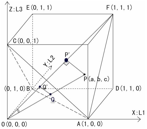
As FA is currently the most popular DTI-derived DAI measurement, FA will be the subject of comparison in assessing the performance of EAR as a new index of anisotropy. Let us first assess more closely what morphological features of a tensor FA really represents. Suppose we have a cube whose 3 axes are designated to be the 3 eigenvalues of a tensor, λ1, λ2, and λ3, each of which ranges from 0 to 1 (Fig. 1). Suppose Dav is the average of the 3 eigenvalues: Dav = (λ1 +λ2 +λ3)/3. Then Eq. (1) can be rewritten as:
| Eq. (10) |
Figure 1.
The Simulated Cube of a Diffusion Tensor Field FA values on the section triangle, ABC, form a representative snapshot of all possible FA values in this cube. This triangle thus provides a context in which we can compare the values of FA with values of EAR for the tensors within the cube. X corresponds to eigenvalue λ1 (L1), Y to λ2 (L2), and Z to λ3 (L3). The tetrahedron OADF occupies 1/6 of the cube, the region in which λ1 ≥ λ2 ≥ λ3. The FA value for the tensor at P(a,b,c) is the trigonometric Sin operator (multiplied by a constant) of the angle between lines PO and OF. Thus, the tensors at P and Q have identical FA values, as do the tensors at P′ and Q′. Indeed, all tensors (except the tensor on origin O) that lie on a single line passing through the origin O will have identical FA values.
Because (Dav, Dav, Dav) is a point location inside the cube (Fig. 1) on the diagonal line segment OF whose equation is X=Y=Z, the numerator in Eq. (10) is actually the distance between the point Λ(λ1,λ2,λ3) under consideration and the line segment OF. More specifically, it is the distance between the point Λ and the point of intersection of the diagonal line OF with the plane that passes through Λ and that is perpendicular to line OF. Moreover, the denominator of Eq. (10) is the distance from the point Λ to the origin O (0,0,0). Therefore, an FA value is actually the trigonometric Sin operator applied to the angle between line OF and the line passing through the origin O and Λ (λ1,λ2,λ3). For instance, P(a, b, c) in Figure 1 is a location with a tensor whose 3 eigenvalues are a, b, and c, and whose FA value is:
| Eq. (11) |
Therefore, all locations on a cone whose tip rests on the origin O (0,0,0) will have the same FA value. Moreover, the section triangle ABC (Fig. 1) is a plane that intersects all possible FA values of a tensor, and therefore the triangle ABC can serve well as a snapshot for surveying all possible FA values, as well as all EAR values, for a similar reason. The triangle ABC is thus a perfect region-of-interest for a general comparison of FA with EAR values.
THEORY
A DAI is most commonly a normalized scalar value ranging from 0 to 1, so that tensors with differing morphologies can be compared and distinguished using the magnitude of this scalar index. To normalize the surface area of a tensor into a common scale as an index for the anisotropy of diffusion, we scale the tensor according to its largest axis, max(λ1, λ2, λ3). Suppose that
| Eq. (12) |
A tensor’s Ellipsoidal Area Ratio (EAR) is then defined in terms of the surface area of a sphere with radius λ -- i.e., with a radius equaling the largest eigenvalue of the tensor:
| Eq. (13) |
The range of possible values of the EAR is [0,1), exactly the same as most DAIs. Moreover, EAR behaviors like the other DAIs, in that it approaches a value of 1.0 when a tensor becomes more needle-like in shape, and it decreases to a value of 0 when the tensor degrades to a sphere.
Because DTI methodologies were developed particularly for the mapping of fiber tracts within the brain, and because nerve fibers are cylindrically symmetrical in their morphology, assessing tensors of cylindrical symmetry is of particular interest [6, 10, 15]. Cylindrical symmetry refers to instances in which a tensor has two identical eigenvalues (e.g. λ2 = λ3) that differ from the remaining eigenvalue (i.e. λ1 ≠λ2). Whereas some investigators use the so-called eigenvalue ratio, λ1/λ2, as a simplified index of cylindrical symmetry[6, 18], DAIs are most commonly examined and compared as indices of anisotropy for tensors with cylindrical symmetry “A” [7, 9, 14, 15], in which
| Eq. (14) |
Although the simplified version of the mathematical approximation of EAR in Eq. (13) reduces to a function of the three eigenvalues of a tensor, similar to the construction of other DAIs, this mathematical approximation of EAR still relates directly to a tensor’s curvature. This measure should therefore provide a more meaningful approximation of diffusion anisotropy compared with the other DAIs, and this should be discernible in measures of image quality, such as SNR and CNR, and in discriminating among tensors of known morphology.
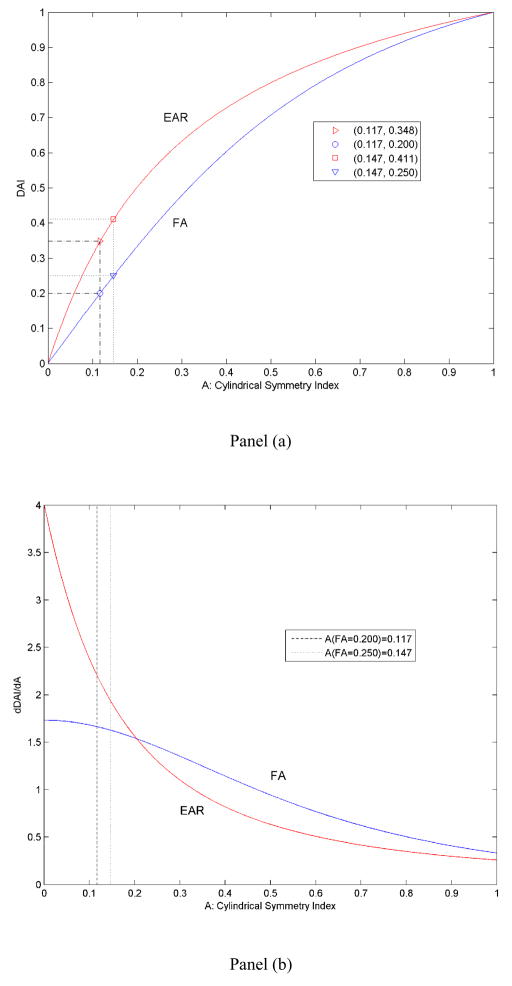
Following studies of other DAIs that were based on cylindrical symmetry A [6, 7, 15, 18], and studies of FA in particular, we too will use tensors having cylindrical symmetry A when measuring the sensitivity of EAR to discriminate tensors of differing morphologies (Fig. 2a). A ranges from a value of −0.5 for oblate tensors (i.e., those that are discoid in shape, when λ1 is near 0), to 0.0 for isotropic tensors (i.e., those that are spherical in shape, in which λ1=λ2=λ3), to 1.0 for prolate tensors (i.e., those that are needle-like in shape, with λ2 and λ3 both close to 0.0). Because the degree of cylindrical symmetry A between 0.0 and 1.0 (for needle-like tensors) is of particular interest in DTI studies[6, 7, 15, 18], DAI is plotted as a function of values of A within this range. In general, EAR acts like a non-linear amplifier of this function for FA, particularly for FAs >0.20 or >0.25 (Fig. 2a), which are at the lower threshold that is typically applied to segment white matter in FA maps and therefore are of particular interest in applied DTI studies. The derivatives with respect to A (Fig 2b) show that in the same segment (where FA > 0.20 or >0.25), EAR is less sensitive to disturbances induced by noise than is FA.
Figure 2.
Comparison of EAR and FA in terms of discriminating tensor morphologies across the range of values for the cylindrical symmetry index A. EAR is overall higher than FA, whereas the derivative of EAR is generally lower than that of FA. Panel (a): DAI values with respect to A; Panel (b): Derivatives of the DAIs with respect to A. The two dashed lines approximate the range within which investigators typically establish the lower threshold of FA values for white matter when segmenting tissue types. The generally lower derivative of EAR compared with that of FA indicates that EAR is less sensitive than is FA to noise perturbation in white matter regions. The boxed insert indicates the A values corresponding to FA values equaling 0.20 and 0.25, the boundary for segmenting white matter and gray matter in FA-maps. (EAR: Ellipsoidal Area Ratio; FA: Fractional Anisotropy; A: Cylindrical symmetry index; DAI: Diffusion)
We calculate SNR and CNR to compare quantitatively the image quality that maps of EAR and FA provide. SNR is the ratio of DAI to noise (noise is the standard deviation σ in the value of the DAI) and CNR is the ratio of contrast (the difference of two DAI values across tensors of differing morphologies) to noise. To compare CNR across differing degrees of anisotropy, we scale CNR with the difference in anisotropy at two DAI values [7]:
| Eq. (15) |
When CNR is measured in the limit of infinitesimal changes in A, this equation becomes:
| Eq. (16) |
To scale the SNR to correct for Rician and normal distributions of noise, as in previous studies [18], we divide by the square-root of 2:
| Eq. (17) |
In certain cases, however, true cylindrical symmetry may be absent (e.g., in biological samples, where eigenvalues are always biased by noise). Therefore, calculations based on cylindrical symmetry may not be feasible. Considering the fact that sRA=A when A>0, CNR can be generalized using sRA instead of A[7]:
| Eq. (18) |
When CNR is measured across tensors that have the same degree of anisotropy, or for tensors across differing tissues, A (i.e., sRA) is either the same or it varies in a range that cannot be factored into the calculation. Therefore, A (or sRA) must be omitted to calculate CNR:
| Eq. (19) |
When the noise σ is similar across differing DAI measurements, CNR is related to SNR as:
| Eq. (20) |
where k is a constant.
Obviously, an increase in SNR need not necessarily increase CNR [4].
MATERIALS AND METHODS
General Comparison of FA and EAR
We first generated a cube of tensor fields taking the three eigenvalues λ1, λ2, and λ3 as 3 variables ranging from 0.0 to 1.0 along the coordinate axes (Fig. 1). As discussed above, we used the section triangle ABC as our study platform because it is a snapshot of all possible FA and EAR values for tensors of varying morphologies, and it spans the largest area inside the cube along the direction perpendicular to the diagonal line OF. This facilitates visual inspection of the differences between the DAIs. The resolution within the cube was 256×256×256. Therefore, each location (x,y,z) in this cube represented a tensor D whose eigenvalues were (x,y,z). We then calculated FA and EAR for each location within the cube, thereby generating one FA volume and one EAR volume across the entire cube. Because the three eigenvalues were interchangeable, only one tetrahedron (constituting 1/6 of the cube) was needed in the cube (e.g. the tetrahedron OADF, in which λ1 ≥ λ2 ≥ λ3, where λ1 = λ2 = λ3 along the line segment OF, λ1 = λ2 along the OD and λ2 = λ3 along AF). In addition, for a more comprehensive view, we used a snapshot of triangle ABC to study the differences between FA and EAR.
Monte Carlo Simulations of Tensors with Cylindrical Symmetry
To compare and evaluate the SNRs and CNRs provided by FA and EAR in the discrimination of tensor morphologies, we performed Monte Carlo simulations with respect to cylindrical symmetry in software package developed in-house using Matlab (version 6.5, MathWorks, Natick, MA). Dav was held constant for all simulations. Using procedures similar to those in prior publications [7, 10, 18, 19], our simulation involved the generation of tensors with differing eigenvalues, the estimation of DW signals, the superposition of differing noise levels on the DW data, the reconstruction of tensors, and the calculation of FA and EAR values:
-
Step_1
Let Doriginal = R•Diag(λ1,λ2,λ3) •RT, where R is a randomized rotation.
-
Step_2
Select a set of k gradient directions, d1, d2, …, dk, di=(di,x, di,y, di,z), that are evenly distributed in 3D space. These will serve as the directions along which the DW images are measured.
-
Step_3
Recover the attenuation ratio of DW measurements along each selected direction di (i= 1,…,k):
-
For each noise-free tensor Doriginal, calculate every Si along the i-th direction:
where
b is the b-value and di is the gradient direction vector
-
-
Step_4Add to Si a noise component having a Gaussian distribution of N(0,σ):
-
Step_5
Reconstruct the Si’s (i= 1,…,k) to a noise-superimposed tensor Dnoise using linear regression
Gaussian-distributed random noise at 1%, 2%, 5%, and 10% levels (relative to the baseline image S0 at b=0) were superimposed on the Si data. These 4 levels of noise were simulated with the corresponding SNRs of 70.7, 35.4, 14.1, and 7.1 for S0 [18]. A total of 200,000 repetitions were simulated for each of the 4 noise levels. FA and EAR were calculated based on the noise-imposed data. Mean DAI values, SNR, CNR were then computed and compared, following the equations defined in the “Theory” section above. CNR values were calculated with differences in A of 0.01.
Human Study
The Monte Carlo simulations provides empirical support for our theoretical analysis addressing only tensors of cylindrical symmetry. To test our theoretical results on an in vivo biological sample containing tensors across a wide range of realistic morphologies, we acquired DW imaging data from five healthy subjects on a GE 3.0-Tesla whole body MRI scanner (General Electric, Milwaukee, WI, USA). Written informed consent was obtained. DW imaging data were acquired along 25 gradient directions plus 3 baseline images without a diffusion-sensitive gradient. Imaging parameters included a b-value = 1000 s/mm2, repetition time (TR) = 17000ms, echo time (TE) = 77 ms, Field of view (FOV) = 240 mm, matrix size = 132 × 128, number of excitation (NEX) = 2. Slice thickness was 2.5 mm at 65 slice locations with no gaps, with a duration of acquisition of 15 minutes. DWI data were first visually inspected to guarantee no obvious motion, and AIR software[20, 21] was used to correct misalignments in the DWI data. We examined the quality of the DW data and found that distortion induced by eddy currents was negligible when compared with the baseline images acquired without the application of a diffusion-sensitive gradient; we therefore elected not to correct for eddy-current distortions. The DWI data were then constructed into tensors using linear regression least-squares-fitting to the logarithmic measurements of the DWIs [10].
To remove non-brain tissue, we first averaged all the DWI data acquired along different gradient directions in a voxel-wise manner and thus obtained a so-called isotropic map for each participant, in which brain tissues have a relatively higher intensity compared with the scalp and other non-brain tissues. A simple intensity threshold removed most non-brain tissue. An automated software tool developed in-house removed residual tissue to provide a brain-tissue mask, which was then used to extract the brain from the raw DW images. Finally, we inspected each image visually and manually removed any remaining non-brain tissue on the raw images.
We used a human brain atlas [22] to identify 10 brain regions for a more detailed examination. These included major fiber pathways within the white matter (e.g. anterior corona radiata, sagittal stratum, corpus callosum, and anterior limb of the internal capsule) (Fig. 3) and several regions in gray matter and cerebrospinal fluid (CSF). An independent operator with two years of experience in brain anatomy manually defined in these structures representative portions that appeared visually homogeneous. Within these regions we compared the mean and standard deviations of EAR and FA, as well as their SNRs and the CNRs across tissues (using Eq. 19), using a Student’s t-test.
Figure 3.
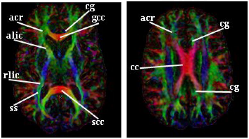
Brain Regions within White Matter Used for Comparison of DAIs acr: anterior corona radiate; ss: sagittal stratum; cc: corpus callosum; scc: splenium of the cc; gcc: genu of the cc; alic: anterior limb of the internal capsule; rlic: retrolenticular part of the internal capsule; cg: cingulum.
| Eq. (21) |
where IMP is the difference between EAR and FA (or the degree of improvement when using EAR relative to FA), and N is the number of samples.
RESULTS
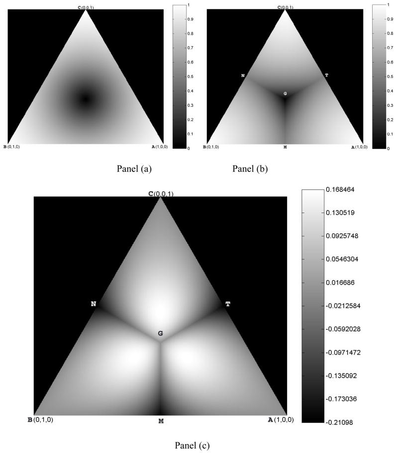
In the snapshots that correspond to the triangle ABC in Figure 1, the FA-map forms concentric circles (Fig. 4a) along the center of the equilateral triangle, whereas the EAR naturally divides the map into 3 parts, each corresponding to the situation in which one of the 3 eigenvalues is more prominent than the other two (e.g. the portion AMGT of Fig. 4b, in which triangle AGM corresponds to the one-sixth portion of the cube in which λ1 ≥λ2 ≥λ3). A line beginning at point A (where λ1 = 1 and λ2 =λ3 = 0) through G (the center of triangle ABC) to N (the mid-point between B and C) corresponds to the region of cylindrical symmetry of measure A, in which λ1 ≠ λ2 = λ3. Moreover, the line segment AG depicts λ1 >λ2 =λ3, and the line segment GN represents λ1 <λ2 =λ3. Subtracting FA from EAR (Fig. 4c) demonstrates that EAR is the superior anisotropy measure in most regions, particularly in regions where tensors are close to cylindrically symmetric (i.e., in regions along line segments AG, BG, and CG). Moreover, these regions of superior anisotropy discrimination are symmetric along these lines of cylindrical symmetry, with the greatest discrimination on line segments in which cylindrical symmetry is positive (i.e., where A > 0). Again, these regions represent tensors that have a cylindrical shape, the tensors that DTI was primarily developed to study. The differences in values of EAR and FA are as large as 0.17.
Figure 4. Comparison of EAR and FA Values on the Section Plane ABC in Fig. 1.
Panel (a) show a map of FA values on plane ABC; FA values form concentric circles along the center of the equilateral triangle. Panel (b) shows a map of EAR values on plane ABC; each of the 3 naturally divided regions (i.e., AMGT, BMGN, CNGT) corresponds to the situation in which one of the three eigenvalues is more prominent than the other two. Triangle AGM corresponds to the one-sixth portion of the cube in which λ1 ≥λ2 ≥λ3. Panel (c) shows a map of the differences obtained when subtracting FA from EAR. The Line segment AGN corresponds to the cylindrical symmetry index A (Fig. 2), on which line segment AG corresponds to the case in which λ1 >λ2 =λ3 and line segment GN to λ1 <λ2 =λ3. The values for EAR are higher than those for FA, particularly in regions along the line segment AG. To the right of each image is a color bar that shows the numerical value corresponding to each gray-scale intensity within the image.
Regions with FA values larger than 0.2 or 0.25 are conventionally segmented as white matter, leaving background noise, CSF, and gray matter within a very limited range of FA values to provide contrast across differing tissues within the image. EAR, in contrast, has rescaled these ranges. The EAR values corresponding to these conventional FA thresholds are 0.35 and 0.41 (Fig. 2a), which has increased by 75% and 64%, respectively, the range of values for CSF and gray matter. As white matter occupies nearly two-thirds (59% to 65%) of the total range of possible EAR values, the allocation of EAR values to differing tissues seems more appropriate than does the allocation of FA.
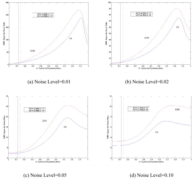
Monte Carlo simulations confirm the impression (from Fig. 2b) that the SNR of EAR is consistently higher than that of FA (Fig. 5), suggesting a relatively greater immunity of EAR to the presence of noise. Although we expected that EAR could be relatively more sensitive to noise when A < 0.2 (Fig. 2b), its SNR was nearly identical to the SNR of FA in this region, perhaps because the tensors were nearly round, rendering the effects of noise on tensor morphology relatively inconsequential. In fact, in regions where the needle-like tensors were very thin (Fig. 5), SNR values of both EAR and FA dropped precipitously, for similar reasons -- i.e., λ2 and λ3 are close to 0 for thin tensors, so that even low noise levels significantly alter anisotropy values. As simulated noise increased from 1% to 10%, SNR curves for EAR and FA diverged, and the SNR of EAR was consistently higher than that of FA (Fig. 5c, d), again demonstrating the greater immunity of EAR to noise. SNR levels lower than 15 are in fact quite typical of DTI data acquired in real-world applications.
Figure 5.
SNR of EAR and FA for Monte Carlo Simulations with 200,000 repetitions in the presence of differing noise levels. (a) Noise level at 1% (~SNR=70.7); (b) Noise level at 2% (~SNR=35.4); (c) Noise level at 5% (~SNR=14.1); (d) Noise level at 10% (~SNR=7.1). The SNR of EAR is overall higher than the SNR of FA, although the values are similar in non-white matter regions (to the left of the dashed lines). With increasing noise levels, the SNR of EAR is consistently higher than that of FA [e.g. in (d)], suggesting that EAR is more robust than is FA to the presence of high noise levels.
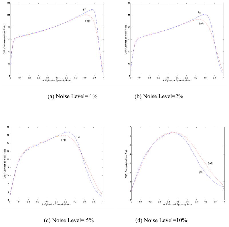
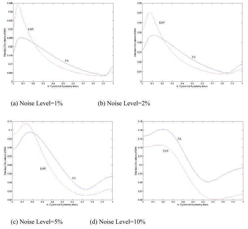
Greater SNR does not necessarily mean greater CNR. In fact, the similar SNR curves at low noise levels accompanied nearly identical CNR curves for EAR and FA in the Monte Carlo simulations (Fig. 6a, b). The SNR of EAR, however, became consistently higher than that of FA at higher noise levels (Fig. 5c, d). Simultaneously, the CNR of EAR surpassed that of FA (Fig. 6c, d) in regions where FA tends to have slightly higher CNR values when noise levels are relatively low. The standard deviations of FA varied much more than did those of EAR in the presence of high noise levels (Fig. 7).
Figure 6. Contrast-to-Noise Ratios (CNR) with a Difference in A (cylindrical symmetry) of 0.01 for EAR and FA Using Monte Carlo Simulations with 200,000 Repetitions.
(a) Noise level 1%; (b) Noise level 2%; (c) Noise level 5%; (d) Noise level 10%. CNRs of EAR and FA are generally similar. When noise increases, the CNR for EAR tends to be higher than that of FA.
Figure 7. Standard Deviation of EAR and FA using Monte Carlo Simulations with 200,000 repetitions.
(a), (b), (c), and (d) are with noise level at 1%, 2%, 5% and 10%, respectively. EAR generally has smaller deviations in white matter regions than does FA. At higher noise levels, EAR tends to have consistently lower deviations than FA.
Similarly, in vivo comparison of FA and EAR in five human subjects (Table 1) indicated that EAR offered significantly better SNRs in white matter regions with confident p-values, ranging from 44–60% (average = 49% across all 8 regions) (Tables 1 & 2). However, improvements in SNR for EAR were not as substantial in gray matter (~ 8%) or CSF (~ 4%) because DAI values in those regions are in the lower end of the range from 0.0 to 1.0; consequently, noise has a relatively greater effect there than in other regions (such as white matter) where DAI values are higher. The standard deviation of EAR is smaller than that of FA in most regions (Fig. 7), and therefore the EAR map appears generally smoother than the FA map (Fig. 8a & b).
Table 1.
Comparison between EAR and FA in important regions of white matter and CSF.
| ROI | Sub ID# | EAR | FA | SNR Improvement (t-score, p-value) | ||||
|---|---|---|---|---|---|---|---|---|
| SNR | Mean EAR | Std. Dev | SNR | Mean FA | Std. Dev | |||
| acr | 1 | 5.74 | 0.683 | 0.084 | 3.93 | 0.561 | 0.101 | 46% |
| 2 | 9.73 | 0.823 | 0.060 | 5.89 | 0.752 | 0.090 | 65% | |
| 3 | 6.97 | 0.790 | 0.080 | 4.20 | 0.703 | 0.118 | 66% | |
| 4 | 14.47 | 0.826 | 0.040 | 9.29 | 0.770 | 0.059 | 56% | |
| 5 | 11.15 | 0.693 | 0.044 | 6.79 | 0.601 | 0.063 | 64% | |
| Average | 9.61 | 6.02 | 59% (14.02, <0.0001) | |||||
| ss | 1 | 7.50 | 0.71 | 0.067 | 4.87 | 0.597 | 0.087 | 54% |
| 2 | 3.74 | 0.724 | 0.137 | 2.54 | 0.635 | 0.177 | 47% | |
| 3 | 10.19 | 0.687 | 0.048 | 6.12 | 0.554 | 0.064 | 67% | |
| 4 | 6.50 | 0.617 | 0.067 | 5.58 | 0.502 | 0.064 | 16% | |
| 5 | 5.62 | 0.74 | 0.093 | 4.10 | 0.641 | 0.111 | 37% | |
| Average | 6.71 | 4.64 | 44% (4.61, 0.005) | |||||
| cc | 1 | 13.28 | 0.847 | 0.045 | 8.21 | 0.784 | 0.068 | 62% |
| 2 | 20.88 | 0.89 | 0.030 | 13.31 | 0.852 | 0.045 | 57% | |
| 3 | 8.77 | 0.842 | 0.068 | 5.51 | 0.776 | 0.100 | 59% | |
| 4 | 9.09 | 0.846 | 0.066 | 5.75 | 0.788 | 0.097 | 58% | |
| 5 | 15.72 | 0.869 | 0.039 | 10.59 | 0.824 | 0.055 | 48% | |
| Average | 13.55 | 8.67 | 57% (21.58, <0.0001) | |||||
| scc | 1 | 17.11 | 0.885 | 0.037 | 10.48 | 0.844 | 0.057 | 63% |
| 2 | 14.26 | 0.859 | 0.043 | 8.55 | 0.805 | 0.067 | 67% | |
| 3 | 31.09 | 0.865 | 0.020 | 19.02 | 0.809 | 0.030 | 63% | |
| 4 | 16.33 | 0.841 | 0.036 | 11.97 | 0.797 | 0.047 | 36% | |
| 5 | 25.79 | 0.908 | 0.025 | 16.28 | 0.883 | 0.038 | 58% | |
| Average | 20.92 | 13.26 | 57% (9.27, 0.0004) | |||||
| gcc | 1 | 18.44 | 0.858 | 0.033 | 11.52 | 0.802 | 0.049 | 60% |
| 2 | 15.52 | 0.878 | 0.040 | 10.98 | 0.838 | 0.054 | 41% | |
| 3 | 11.88 | 0.834 | 0.050 | 7.08 | 0.767 | 0.076 | 68% | |
| 4 | 10.82 | 0.817 | 0.053 | 6.62 | 0.739 | 0.079 | 63% | |
| 5 | 14.71 | 0.814 | 0.039 | 10.10 | 0.746 | 0.052 | 46% | |
| Average | 14.27 | 9.26 | 56% (9.63, 0.0003) | |||||
| alic | 1 | 17.59 | 0.819 | 0.033 | 10.32 | 0.750 | 0.051 | 70% |
| 2 | 6.75 | 0.804 | 0.084 | 4.34 | 0.738 | 0.120 | 56% | |
| 3 | 10.18 | 0.805 | 0.056 | 6.27 | 0.726 | 0.082 | 62% | |
| 4 | 9.19 | 0.816 | 0.063 | 5.79 | 0.758 | 0.093 | 59% | |
| 5 | 11.68 | 0.825 | 0.050 | 7.68 | 0.757 | 0.070 | 52% | |
| Average | 11.08 | 6.88 | 60% (17.60, <0.0001) | |||||
| rlic | 1 | 10.02 | 0.684 | 0.048 | 7.51 | 0.585 | 0.055 | 33% |
| 2 | 9.80 | 0.806 | 0.058 | 5.98 | 0.728 | 0.086 | 64% | |
| 3 | 6.57 | 0.775 | 0.083 | 3.94 | 0.681 | 0.122 | 67% | |
| 4 | 9.05 | 0.806 | 0.063 | 6.92 | 0.750 | 0.077 | 31% | |
| 5 | 8.40 | 0.634 | 0.053 | 6.71 | 0.508 | 0.054 | 25% | |
| Average | 8.77 | 6.21 | 44% (4.43, 0.006) | |||||
| cg | 1 | 8.61 | 0.781 | 0.064 | 5.39 | 0.698 | 0.091 | 60% |
| 2 | 9.67 | 0.825 | 0.060 | 6.26 | 0.759 | 0.086 | 35% | |
| 3 | 10.86 | 0.871 | 0.057 | 7.17 | 0.822 | 0.081 | 51% | |
| 4 | 6.67 | 0.791 | 0.084 | 4.13 | 0.712 | 0.122 | 62% | |
| 5 | 7.63 | 0.791 | 0.073 | 4.95 | 0.708 | 0.101 | 54% | |
| Average | 8.69 | 5.58 | 52% (9.80, 0.0003) | |||||
acr: anterior corona radiate; ss: sagittal stratum; cc: corpus callosum; scc: splenium of the cc; gcc: genu of the cc; alic: anterior limb of the internal capsule; rlic: retrolenticular part of the internal capsule; cg: cingulum. Std. Dev.: Standard Deviation; ROI: region of interest
Table 2.
Comparison between EAR and FA of the 3 tissue types.
| ROI | EAR | FA | SNR Improvement | |||||
|---|---|---|---|---|---|---|---|---|
| SNR | Mean EAR | Std. Dev | SNR | Mean FA | Std. Dev | |||
| WM | 1 | 6.56 | 0.811 | 0.087 | 4.39 | 0.739 | 0.119 | 49% |
| 2 | 6.98 | 0.841 | 0.085 | 4.78 | 0.784 | 0.116 | 46% | |
| 3 | 7.37 | 0.824 | 0.079 | 4.63 | 0.750 | 0.115 | 59% | |
| 4 | 6.19 | 0.807 | 0.092 | 4.23 | 0.738 | 0.123 | 46% | |
| 5 | 7.68 | 0.838 | 0.077 | 5.25 | 0.781 | 0.105 | 46% | |
| Average | 6.96 | 0.824 | 0.084 | 4.66 | 0.758 | 0.116 | 49% | |
| GM | 1 | 2.81 | 0.251 | 0.063 | 2.71 | 0.157 | 0.041 | 4% |
| 2 | 4.76 | 0.281 | 0.042 | 4.14 | 0.180 | 0.031 | 15% | |
| 3 | 2.87 | 0.263 | 0.065 | 2.87 | 0.163 | 0.040 | 0% | |
| 4 | 2.11 | 0.220 | 0.074 | 1.79 | 0.143 | 0.057 | 18% | |
| 5 | 3.12 | 0.254 | 0.058 | 3.05 | 0.160 | 0.037 | 2% | |
| Average | 3.13 | 0.254 | 0.060 | 2.91 | 0.161 | 0.041 | 8% | |
| CSF | 1 | 2.38 | 0.141 | 0.042 | 2.28 | 0.080 | 0.025 | 4% |
| 2 | 1.88 | 0.153 | 0.058 | 1.93 | 0.084 | 0.031 | −3% | |
| 3 | 2.10 | 0.155 | 0.052 | 2.12 | 0.086 | 0.029 | 0% | |
| 4 | 1.73 | 0.140 | 0.057 | 1.47 | 0.080 | 0.038 | 18% | |
| 5 | 2.15 | 0.148 | 0.048 | 2.06 | 0.083 | 0.028 | 4% | |
| Average | 2.05 | 0.147 | 0.051 | 1.97 | 0.083 | 0.030 | 4%~5% | |
WM: white matter (the combination of all 8 ROIs in Table 1); GM: gray matter; CSF: cerebral-spinal fluid; EAR: ellipsoidal area ratio; FA: fractional anisotropy; SNR: signal-to-noise ratio.
Figure 8. In vivo DAI Maps in a Human Subject.
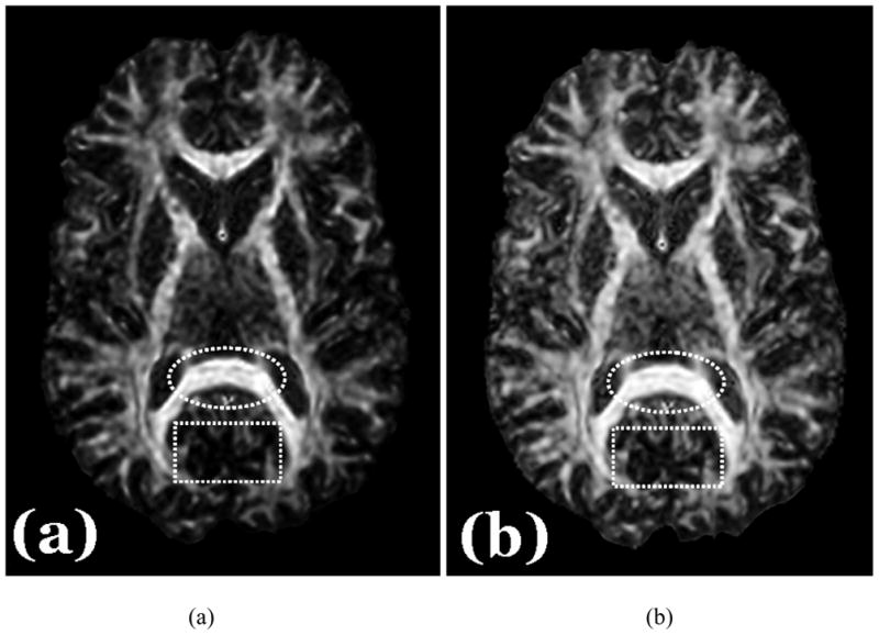
(a) FA map; (b) EAR map. EAR typically provides a CNR within tissues that is similar to that for FA, although EAR has relatively greater SNR. Consequently, the EAR map appears smoother than the FA map (e.g. the region of the corpus callosum within the dotted circle). EAR, on the other hand, provides a higher CNR across differing tissue types (white matter vs. other tissues), producing clearer delineation of small structures in regions of mixed tissue types (e.g. the small structural details in the dashed rectangle). Better CNR should not be confused with the visibility of the major fiber pathways. Thus in the FA map, only the skeletons of major fiber pathways (a portion of the white matter) are prominently visible, because FA does not offer a well-balanced CNR for all ranges of anisotropy values across white matter and other tissue types. In contrast, almost all white matter regions are visible in the EAR map.
The CNR with respect to a difference in A of 0.01 assessed the contrast characteristics of DAIs for tensors with slightly differing shapes (Fig. 6). For the routine processing and segmentation of DT images, measuring CNR across differing tissues containing tensors with a wide variety of shapes is preferred. We found in human data that EAR offers better CNR between white matter and other tissue types than does FA (Table 3 and Fig. 8), which subsequently yielded better visibility of anatomical details in the EAR compared with FA maps (Fig 9), particularly when the color map of the unit principal directions of the tensors was scaled by the DAIs. The CNR for EAR across gray matter and CSF was nearly identical to that for FA (1.11 versus 1.26), although EAR did offer better SNR in these regions.
Table 3.
CNR of White Matter versus Other Tissue Types
| Tissues | CNR based on EAR | CNR based on FA | CNR Improvement |
|---|---|---|---|
| WM vs. GM | 5.67 | 4.97 | 14~15% |
| WM vs. CSF | 6.89 | 5.63 | 21~22% |
Figure 9. In vivo Color Maps of the Principal Direction (PD) of Tensors in a Human Subject.
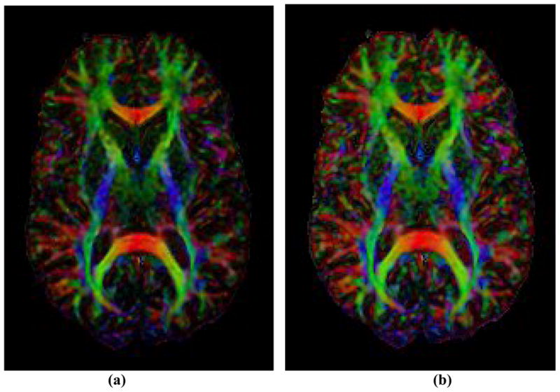
(a) Color map based on FA; (b) Color map based on EAR. Compared with the map using FA values, the color map of principal directions is enhanced when using EAR values. Anatomical details are clearer and more discernible. Color schema: red for PDs oriented in horizontal directions; green for vertical; and blue for perpendicular to the viewing plan.
DISCUSSION
We have developed a new index, EAR, for the measurement of the anisotropy of diffusion. We propose it as an attractive alternative to the more routine use of FA in measuring anisotropy. EAR does not require the sorting of eigenvalues, and it is therefore free from the bias caused by such sorting [23, 24]. Although a complete and exact comparison of EAR with FA across all possible tensor morphologies is impossible, we have provided a general analysis (Fig. 1) and an overall comparison (Fig. 4) of the behavior and performance of these two DAIs. Moreover, we have adopted the convention of studying the performance of the two DAIs in discriminating tensors of cylindrical symmetry, the types of tensors that are deemed most important and most representative in studying white matter of the brain. Both our simulation and in vivo studies demonstrated that EAR may be preferred over FA as a DAI. The superior performance of EAR was evident even in our study of five real-world datasets that indeed did encompass tensors of all possible realistic morphologies. Monte Carlo simulations approximated noise conditions found in typical DTI experiments and found that EAR outperforms FA in terms of SNR in the presence of high noise levels (5% noise, SNR=14.1; 10% noise, SNR=7.1) similar to the levels present in real-world datasets. Indeed, the superior performance of EAR was confirmed in vivo. Although the CNR of EAR for tensors of cylindrical symmetry within the same tissue type was similar to that of FA in the presence of low noise levels, EAR provided superior CNR when noise levels were high. Moreover, the CNR across tissue types in real-world datasets was generally superior statistically for EAR compared with FA. This improved CNR provides a decided advantage for image segmentation and other procedures that depend on tissue contrast. Thus, the robustness of EAR to noise seems to make it preferable to FA for use in discriminating tensors of differing morphologies.
EAR also offers a number of advantages over FA for image processing. FA values for the image background, CSF, and gray matter fall within a narrow range, typically below 0.25, when the range of possible values for FA is from 0.0 to 1.0. The narrow range of FA values for portions of the image other than white matter greatly complicates the separation of gray matter, CSF, and image background from one another. In contrast, these regions within the EAR maps occupy a wider range of values, although values for white matter still occupy the majority (>59%) of the total range, which is appropriate for an imaging modality that is used primarily to study fiber organization in white matter. The wider range of EAR values for differing tissue types and background noise will allow for easier and more precise segmentation of differing brain tissues using measures of anisotropy.
EAR may benefit fiber tracking, as well. EAR compared with FA typically yields larger measures of diffusion anisotropy in white matter (Fig. 2). The vector for the Principal Direction (PD) of a tensor is therefore estimated with greater confidence in white matter when using EAR rather than FA, thus improving inferences regarding orientation of local fibers and thereby increasing the likelihood of successful fiber tracking in tractography studies. Previous efforts in fiber tracking have applied a nonlinear logarithmic operator of FA [25] to enhance nonlinearly the length of the vectors within the PDs of tensors. Enhancing the vectors through the use of EAR may achieve the same goal for fiber tracking without incurring the added computational demands.
Finally, EAR relates directly to the surface area of a tensor’s ellipsoid. Whereas its calculation with full precision is readily available but computationally expensive (Eq. 7), we adopted its approximation with ultrafine error (Eq. 9). Although this simplification has been reduced to the use of only the three eigenvalues λ1, λ2, and λ3, and thus it appears similar in form to the other DAIs, the resemblance of EAR to the other DAIs is only superficial, as the others are not supported naturally by a simple mathematical construct and are not as amenable to a simple geometric interpretation as is EAR.
In conclusion, EAR is a DAI that has a number of advantages over the other DAIs that are currently in most common use. EAR is a precise and intuitive approximation of the curvature of a tensor’s ellipsoid that encodes directly the biologically relevant characteristics of diffusion that a tensor is intended to measure. Therefore, EAR is likely to enhance substantially the measurement of diffusion anisotropy and its application to the study of tissue organization and fiber tracking in the human brain.
Acknowledgments
The authors thank Dr. Jason Royal for his time, editorial comments, and suggestions that enhanced the technical presentation of this paper. This work was supported by a grant from NARSAD, NIBIB grant 1R03EB008235-01A1, NIDA grant DA017820, NIMH grants MH068318 and K02-74677, a grant from the Simons Foundation, and the Suzanne Crosby Murphy Endowment at Columbia University College of Physicians and Surgeons.
Footnotes
http://home.att.net/~numericana/answer/ellipsoid.htm#thomsen; In lieu of traditional peer review, this approximation has been discussed and analyzed by Sigma Xi mathematician David W. Cantrell in the sci.math newsgroup (search with keywords ‘knud thomsen’ and ‘ellipsoid’).
Publisher's Disclaimer: This is a PDF file of an unedited manuscript that has been accepted for publication. As a service to our customers we are providing this early version of the manuscript. The manuscript will undergo copyediting, typesetting, and review of the resulting proof before it is published in its final citable form. Please note that during the production process errors may be discovered which could affect the content, and all legal disclaimers that apply to the journal pertain.
References
- 1.Schwartzman A, Dougherty RF, Taylor JE. A Log-Normal Distribution and Two-Sample Tests for the Full Diffusion Tensor. Human Brain Mapping 11th Meeting; 2005; Toronto. [Google Scholar]
- 2.Schwartzman A, Dougherty RF, Taylor JE. Cross-Subject Comparison of Principal Diffusion Direction Maps. Magnetic Resonance in Medicine. 2005;53:1423–1431. doi: 10.1002/mrm.20503. [DOI] [PMC free article] [PubMed] [Google Scholar]
- 3.Xu D, Mori S, Shen D, Zijl PCMv, Davatzikos C. Spatial Normalization of Diffusion Tensor Fields. Magnetic Resonance in Medicine. 2003;50:175–182. doi: 10.1002/mrm.10489. [DOI] [PubMed] [Google Scholar]
- 4.Hasan KM, Alexander AL, Narayana PA. Does fractional anisotropy have better noise immunity characteristics than relative anisotropy in diffusion tensor MRI? An analytical approach. Magnetic Resonance in Medicine. 2004;51:413–417. doi: 10.1002/mrm.10682. [DOI] [PubMed] [Google Scholar]
- 5.Papadakis NG, Xing D, Houston G, Smith J, Smith M, James M, Parsons A, Huang C, Hall L, Carpenter T. A Study of Rotationally Invariant and Symmetric Indices of Diffusion Anisotropy. Magn Res Imaging. 1999;17:881–892. doi: 10.1016/s0730-725x(99)00029-6. [DOI] [PubMed] [Google Scholar]
- 6.Wang JJ, Chao TC, Wai YY, Hsu YY. Novel Diffusion Anisotropy Indices: An Evaluation. Journal of Magnetic Resonance Imaging. 2006;24:211–217. doi: 10.1002/jmri.20616. [DOI] [PubMed] [Google Scholar]
- 7.Kingsley PB, Monahan WG. Contrast-to-noise ratios of diffusion anisotropy indices. Magnetic Resonance in Medicine. 2005;53(4):911–918. doi: 10.1002/mrm.20433. [DOI] [PubMed] [Google Scholar]
- 8.Alexander AL, Hasan K, Kindlmann G, Parker D, Tsuruda J. A Geometric Analysis of Diffusion Tensor Measurements of the Human Brain. Magnetic Resonance in Medicine. 2000;44:283–291. doi: 10.1002/1522-2594(200008)44:2<283::aid-mrm16>3.0.co;2-v. [DOI] [PubMed] [Google Scholar]
- 9.Armitage PA, Bastin ME. Selecting an appropriate anisotropy index for displaying diffusion tensor imaging data with improved contrast and sensitivity. Magnetic Resonance in Medicine. 2000;44:117–121. doi: 10.1002/1522-2594(200007)44:1<117::aid-mrm17>3.0.co;2-d. [DOI] [PubMed] [Google Scholar]
- 10.Pierpaoli C, Basser PJ. Toward a quantitative assessment of diffusion anisotropy. Magnetic Resonance Med. 1996;36:893–906. doi: 10.1002/mrm.1910360612. [DOI] [PubMed] [Google Scholar]
- 11.Bastin ME, Armitage PA, Marshall I. A Theoretical Study of the Effect of Experimental Noise on the Measurement of Anisotropy in Diffusion Imaging. Magnetic Resonance Imaging. 1998;16:773–785. doi: 10.1016/s0730-725x(98)00098-8. [DOI] [PubMed] [Google Scholar]
- 12.Basser PJ. Inferring microstructural features and the physiological state of tissues from diffusion-weighted images. NMR Biomed. 1995;8:333–344. doi: 10.1002/nbm.1940080707. [DOI] [PubMed] [Google Scholar]
- 13.Basser PJ, Pierpaoli C. Microstructural and Physiological Features of Tissues Elucidated by Quantitative-Diffusion-Tensor MRI. Journal of Magnetic Resonance Imaging. 1996;111(Series B):209–219. doi: 10.1006/jmrb.1996.0086. [DOI] [PubMed] [Google Scholar]
- 14.Conturo TE, McKinstry RC, Akbudak E, Robinson BH. Encoding of anisotropic diffusion with tetrahedral gradients: a general mathematical diffusion formalism and experimental results. Magnetic Resonance in Medicine. 1996;35:399–412. doi: 10.1002/mrm.1910350319. [DOI] [PubMed] [Google Scholar]
- 15.Ulug AM, van Zijl PC. Orientation-Independent Diffusion Imaging Without Tensor Diagonalization: Anisotropy Definitions Based on Physical Attributes of the Diffusion Ellipsoid. Journal of Magnetic Resonance Imaging. 1999;9:804–813. doi: 10.1002/(sici)1522-2586(199906)9:6<804::aid-jmri7>3.0.co;2-b. [DOI] [PubMed] [Google Scholar]
- 16.Klamkin MS. Elementary approximations to the area of n-dimensional ellipsoids. The American Mathematical Monthly. 1971;78:280–283. [Google Scholar]
- 17.Klamkin MS. Corrections to “Elementary approximations to the area of n-dimensional ellipsoids. The American Mathematical Monthly. 1976;83:478. [Google Scholar]
- 18.Skare S, Li T, Nordell B, Ingvar M. Noise considerations in the determination of diffusion tensor anisotropy. Magn Reson Imaging. 2000;18(6):659–69. doi: 10.1016/s0730-725x(00)00153-3. [DOI] [PubMed] [Google Scholar]
- 19.Xu D, Hao X, Bansal R, Plessen JK, Peterson BS. Seamless Warping of Diffusion Tensor Fields. IEEE Transactions on Medical Imaging. 2008 doi: 10.1109/TMI.2007.901428. (accepted) [DOI] [PMC free article] [PubMed] [Google Scholar]
- 20.Woods RP, Grafton ST, Holmes CJ, Cherry SR, Mazziotta JC. Automated image registration: I. General methods and intrasubject, intramodality validation. Journal of Computer Assisted Tomography. 1998;22(1):139–52. doi: 10.1097/00004728-199801000-00027. [DOI] [PubMed] [Google Scholar]
- 21.Woods RP, Grafton ST, Watson JD, Sicotte NL, Mazziotta JC. Automated image registration: II. Intersubject validation of linear and nonlinear models. Journal of Computer Assisted Tomography. 1998;22(1):153–65. doi: 10.1097/00004728-199801000-00028. [DOI] [PubMed] [Google Scholar]
- 22.Mori S, Wakana S, Nagae-Poetscher LM, Van Zijl PC. MRI Atlas of Human White Matter. 2005. Elseview. [DOI] [PubMed] [Google Scholar]
- 23.Martin KM, Papadakis NG, Huang CL-H, Hall LD, Carpenter TA. The Reduction of The Sorting Bias in The Eigenvalues of The Diffusion Tensor. Magnetic Resonance Imaging. 1999;17(6):893–901. doi: 10.1016/s0730-725x(99)00021-1. [DOI] [PubMed] [Google Scholar]
- 24.Basser PJ, Pajevic S. Statistical Artifacts in Diffusion Tensor MRI (DT-MRI) Caused by Background Noise. Magnetic Resonance in Medicine. 2000;44:41–50. doi: 10.1002/1522-2594(200007)44:1<41::aid-mrm8>3.0.co;2-o. [DOI] [PubMed] [Google Scholar]
- 25.Zhu H, Xu D, Raz A, Hao X, Zhang H, Kangarlu A, Bansal R, Peterson BS. A Statistical Framework for the Classification of Tensor Morphologies in Diffusion Tensor Images. Magnetic Resonance Imaging. 2006;24(5):569–582. doi: 10.1016/j.mri.2006.01.004. [DOI] [PMC free article] [PubMed] [Google Scholar]


