

Abstract
A new way to use wide-angle x-ray solution scattering to study protein-ligand binding is presented. First, scattering patterns are measured at different protein and ligand concentrations. Multivariate curve resolution based on singular value decomposition and global analysis is applied to estimate the binding affinities and reference patterns (i.e., the scattering patterns of individual components). As validated by simulation, Bayesian confidence intervals provide accurate uncertainty estimates for the binding free energies and reference patterns. Experimental results from several protein-ligand systems demonstrate the feasibility of the approach, which promises to expand the role of wide-angle x-ray scattering as a quantitative biophysical tool.
Introduction
X-ray solution scattering is an important technique in molecular biophysics. Small-angle x-ray solution scattering (SAXS) is frequently used to measure the radius of gyration (1), estimate the pair distribution function (2), and compute low-resolution shape envelopes (3–5) of biological macromolecules. Wide-angle x-ray solution scattering (WAXS) data contain information about the protein fold (6) and can detect the response of protein structural ensembles to various perturbations, including macromolecular crowding (7) and ligand binding (8–12). It is becoming increasingly common to combine x-ray solution scattering with molecular modeling and other biophysical techniques to assess and refine models for structures and structural ensembles (13–21).
A significant challenge in the interpretation of x-ray solution scattering data is the need to isolate signals from different species. Solutions often contain a mixture of species (e.g., a protein may exist both as a monomer and dimer in solution), and the observed scattering patterns are a linear combination of scattering from each species. This may be written generically as
| (1) |
In this expression, D is an data matrix with M measurements and A scattering angles, in which an element refers to the scattering intensity for measurement m at scattering angle bin a. C is an matrix of concentrations for each species, where K is the number of species, and R is a matrix of K reference patterns. Finally, ε is an residual matrix whose elements may be attributed to measurement noise.
Estimating C and R to reproduce D while minimizing an objective function for ε is useful beyond x-ray scattering, with applications, for example, to various spectroscopic techniques. In the broader chemometrics literature, this is known as multivariate curve resolution (22). From the perspective of data analysis, the simplest way to achieve multivariate curve resolution is by experimental design, i.e., the contribution of a precisely matched buffer obtained by dialysis can be directly subtracted, a solution can be purified so that there is only one macromolecule, or a protein can be saturated with ligand such that, to a very good approximation, it exists only in the holo form. Due to experimental constraints, however, these options may be unavailable. For example, equilibrium dialysis is precluded in time-resolved experiments or experiments involving short-lived proteins. Solubility can limit one’s ability to purify a molecule or saturate a receptor. In such cases, multivariate curve resolution must be accomplished mathematically.
Multivariate curve resolution methods can be broadly categorized into two forms: soft modeling and hard modeling (22). In soft modeling, neither C nor R is modeled a priori; an attempt is made to discern both directly from the data. This approach has the advantage of making few assumptions, but resulting estimates are often not precise or unique, and thus conclusions may be ambiguous. In contrast, hard modeling assumes a specific physiochemical model for C. Hard modeling makes the most sense when there is a strong justification for C, or when one needs to assess whether various models for C are supported by the data. It allows one to estimate parameters for C, such as time constants or binding affinities, and usually provides more unique and precise answers for R. (Another way to analyze x-ray scattering data is to predict R based on molecular models and use experimental data to estimate C (23); however, this promising approach is not actually curve resolution because reference patterns are determined before the data are analyzed.) To our knowledge, x-ray solution scattering data from biological macromolecules have only been interpreted with a variety of physiochemical hard models. For time-resolved data, kinetic models have been used (10,24,25). Thermodynamic models for oligomerization (26,27), equilibrium unfolding (28,29), and protein-micelle interactions (30) have all been applied to SAXS.
In this work, we apply a stoichiometric hard model to study the noncovalent association between a macromolecule and a small-molecule ligand. The experiments and data analysis strategy presented here were chosen to provide a methodological foundation for future experiments on more complex macromolecular systems. Consequently, we estimate the contributions from protein, ligand, and buffer from a global analysis of all collected scattering patterns rather than performing an initial background subtraction of scattering from a precisely matched buffer from scattering from protein solutions. Processing strategies are initially applied to simulated data and assessed for their ability to provide reasonable Bayesian confidence intervals (CIs) for binding free energies and R. The best methods for simulated data are then applied to interpret experimental WAXS patterns measured at different protein and ligand concentrations. As will be apparent, nonidealities in the experimental data lead to results that are not always optimized when the same parameters employed for the simulated data are used. In response to these observations, we report the effect of changes in experimental and analytical parameters on the derived results, with the goal of identifying areas of experimental design that are most relevant for obtaining accurate results.
Materials and Methods
Sample preparation
For each protein-ligand system, we prepared solutions at a variety of protein and ligand concentrations. Although our analysis is valid for a wide range of protein concentrations, we only prepared solutions in which protein was absent or added at one specific concentration; varying protein concentrations may result in macromolecular crowding effects (7) that are not readily explained by the binding model. Because ligands are smaller and less likely to cause crowding, we added them at concentrations ranging from less than equimolar to a severalfold excess relative to the respective protein concentrations.
Hen egg white lysozyme (subsequently referred to as lysozyme; catalog No. L6876) and N-acetyl-D-glucosamine (NAG; catalog No. A8625) were purchased from Sigma-Aldrich (St. Louis, MO). (NAG)2 (catalog No. OD00769) and (NAG)3 (catalog No. ODT06497) were purchased from Carbosynth Ltd. (Compton, UK). The lysozyme and its ligands were dissolved in 0.02 M sodium acetate (pH 4.5) and 0.1 M NaCl. Solutions (180 mL) containing either 0 or 1 mM (14.3 mg/mL) lysozyme and 0, 0.1, 0.2, 0.4, 0.6, 0.8, 1, 1.5, 2, 4, 10, 20, or 40 mM NAG; 0.1, 0.2, 0.4, 0.6, 0.8, 1, 1.5, 2, 4, or 10 mM (NAG)2; or 0.1, 0.2, 0.4, 0.6, 0.8, 1, 2, or 4 mM (NAG)3 were prepared from more concentrated stock solutions.
Human galectin-1 (subsequently referred to as galectin; UniProt P09382) was recombinantly overexpressed in Escherichia coli with the pMCSG7 expression vector (31) by the technical staff of the Makowski laboratory. A His-tag was used for purification and subsequently cleaved by TEV protease. D-lactose monohydrate (lactose) was purchased from Sigma-Aldrich (catalog No. 61345) and dissolved in PBS. Solutions (180 mL) containing either 0 or 0.4 mM (5.9 mg/mL) galectin and 0, 0.2, 0.4, 0.6, 1, 2, and 8 mM lactose were prepared from stock solutions of 0.75 mM (11 mg/mL) galectin and 4 and 40 mM stock solutions of lactose, all in PBS.
Alcohol dehydrogenase (ADH) from baker’s yeast (catalog No. A7011) and β-nicotinamide adenine dinucleotide (NAD+; catalog No. N8535) were purchased from Sigma-Aldrich and dissolved in buffer containing 100 mM citrate (pH 6.0) and 1 mM Zn acetate. To minimize residual cofactor from ADH, the buffer was exchanged in centrifugal filter tubes until at least a 1000-fold dilution was reached. Solutions (180 mL) containing either 0 or 0.18 mM (25 mg/mL) ADH and 0, 0.09, 0.13, 0.18, 0.36, 0.71, 1.42, or 1.77 mM NAD+ were prepared from stock solutions of 0.25 mM (35 mg/mL) ADH and 0.15, 1.5, and 15 mM NAD+ in the appropriate buffer.
Stock protein concentrations were estimated by absorbance at 280 nm using parameters from ProtParam (32).
WAXS
WAXS data were collected at the BioCAT undulator beam line (18ID) at the Advanced Photon Source, Argonne, IL (33). Experimental data were collected as previously described (see Makowski et al. (11) and Supporting Material), with exposure levels such that the effect of radiation damage on radiosensitive test proteins was undetectable (34). Outlier patterns, generated due to passage of small bubbles through the x-ray beam during the exposure, were removed.
We averaged two-dimensional scattering patterns circularly using Fit2D version 14.101 (35,36), applying a polarization correction with polarization factor of 0.99, and binning measured intensities at each pixel into 1000 equally spaced scan bins with a maximum angle of 28°. In this work, we will also refer to angles by , where λ is the incident x-ray wavelength of , and .
Scattering patterns were normalized by the incident photon count. The incident photon count was measured by both the integrated beam flux from the ion chamber and the total photon count, summed over all pixels, in the MAR165 2k × 2k CCD detector. The former is more consistent across different conditions, because it does not depend on the sample, but the latter appears to be more precise. Hence, ion chamber measurements were used to calibrate the pixel sum in each equivalent exposure by ordinary linear least-squares regression, and the calibrated pixel sum was used for normalization.
Normalized scattering patterns were stored in two data matrices: D (with dimensions ) and (with dimensions ). In D, each row is the average of all scattering patterns collected under the same conditions. In , each row is a scattering pattern from an individual x-ray exposure. Henceforth, M will refer to the number of conditions and will refer to the number of individual x-ray exposures.
The presence of a beam stop, which is required to prevent incident beam damage to the detector, necessitated truncation of data below . Because solvent structure changes observed at wider angles are not linear effects explained by our concentration model, scattering patterns were also truncated above a maximum .
The nonlinearity is due to the concentration dependence of the partial specific volume of the ligand (37), which gives rise to a modest but observable nonlinearity in scattering from the buffer. In the “Scattering angles” section below, we explore the effect of varying this cutoff and find that (leaving angular bins in the data matrices) yields reasonable results for all systems studied here; this cutoff is used in all other sections.
Stoichiometric hard model
Our stoichiometric hard model is based on a noncovalent association between a macromolecule M and ligand L to form a complex :
| (2) |
The equilibrium concentrations of these species, denoted with square brackets, depend on the dissociation constant:
| (3) |
or, equivalently, the binding free energy:
| (4) |
where R is the gas constant, T is the temperature in degrees Kelvin, and is the standard concentration (1 M) included so that the term inside the logarithm is dimensionless.
Let and be the total concentrations of macromolecule and ligand, respectively, before formation of the macromolecule-ligand complex. Then , , and by the quadratic equation,
| (5) |
For each measurement, the concentration matrix contains four columns ,
| (6) |
corresponding to background (air, capillary, and solvent), free ligand, free macromolecule (apo), and the macromolecule-ligand complex (holo), respectively. We set the arbitrary constant to be of the same order of magnitude as the other contributions. The original concentrations are assumed to be determined by experimental design (there is no concentration error), and thus C has only one free parameter, .
Another possible procedure is to subtract the background before analysis and use a three-species model with , , and . However, because solvent scattering is intense at wider angles, accurate background subtraction is challenging with WAXS. It is unclear how much solvent is displaced by a particular combination of solutes, and what fraction of the background may be attributed to solvent, capillary, or air. Hence, we find a four-species model to be superior to a three-species model.
The four-species model has the additional benefit that the obtained reference patterns for the macromolecule, ligand, and macromolecule-ligand complex (which constitute three rows of R) are excess intensities that may be predicted from models of structural ensembles (38) (although obtaining accurate ensembles remains challenging because of current limitations in molecular-mechanics force fields and configurational sampling). Park et al. (38) defined an excess intensity pattern as the difference between the scattering patterns of a macromolecule and its buffer, and described how it can be predicted from the structural emsemble of a macromolecule in explicit solvent. Denoting the nth row of R with a subscript, , the scattering patterns of the macromolecule and buffer are and , respectively. Thus, the reference pattern for the macromolecule, , is proportional to the excess intensity. By analogy, we can see that the reference pattern for the ligand, , is proportional to the difference between the scattering pattern of a free ligand in buffer and the buffer without ligand. Finally, is proportional to the difference between the macromolecule-ligand complex and the buffer; both and can be estimated based on the theoretical framework in Park et al. (38).
Multivariate curve resolution
Given the data matrix D and concentration matrix C, the reference matrix R may be obtained by various forms of linear regression. Ordinary least squares minimizes the sum of squares of the residual matrix:
| (7) |
Although it is straightforward, this treatment neglects correlation and heteroskedasticity.
Although photon counts from adjacent pixels of a CCD detector are somewhat correlated, this effect is highly local; it is reasonable to approximate that measurement errors for different angular bins in x-ray scattering patterns are uncorrelated. However, the variances of different angular bins, which are inversely related to the number of pixels in each bin, differ substantially. This heteroskedasticity may be accounted for by a weighted least-squares method that minimizes
| (8) |
where is the standard deviation (SD) of measurement m at angular bin a.
Although is it possible to estimate based on the noise performance of individual pixels on the detector, there are a number of other sources of error (e.g., polarization and slow drift of the synchrotron beam, the noise performance of the ion chamber, and scattering and absorbance by the capillary) that are difficult to treat. Because we collected multiple exposures for each condition, we instead estimated the matrix based on the sample variance of integrated scattering patterns:
| (9) |
where
| (10) |
and is an indicator function that is one if measurements m and n are from the same solution condition, and is zero otherwise.
With a fairly limited number of samples per condition, it is useful to apply a shrinkage approximation. In all of our x-ray scattering experiments, we observed the largest heteroskedasticity in the presence or absence of protein, and the variance was larger in solutions with protein than in solutions without it. In light of this error structure, we estimated the variance of an exposure by
| (11) |
in which equals one if condition a contains protein, and zero otherwise. is the opposite indicator function (i.e., it equals one if condition a does not contain protein, and zero if it does).
We estimated the reference pattern matrix R using the lscov function in MATLAB 2011b (The MathWorks, Natick, MA) and 1), ordinary least squares; 2) weighted least squares, weighed by the inverse of the sample variance (Eq. 9); or 3), weighted least squares, weighed by the inverse of the shrinkage approximation variance (Eq. 11).
Bayesian CIs
Least-squares regression minimizes for a particular concentration matrix C, but how does one choose C? Because C depends solely on the unknown parameter (recall our assumption that concentrations are exact), we may simply choose a value of that leads to a C that minimizes a (weighted) residual matrix. Indeed, this is a reasonable point estimate.
We would also like to estimate CIs for the parameter . Toward this end, note that if is uncorrelated Gaussian noise with known variance, the log likelihood (excluding the normalizing constant) of observing a particular data set is
| (12) |
Because ε is uniquely obtained by weighted least-squares linear regression, it implicitly depends on D.
Applying Bayes’ law, , and an uninformative Gaussian prior, , we obtain a posterior probability (excluding the normalizing constant) for :
| (13) |
Because the model has only one parameter, we may evaluate CIs for without extensive sampling from . Instead, we apply a grid-based approach, evaluating between and 0 kcal/mol at intervals of 0.05. Then for a smaller region , between the minimal and maximal i for which , where has the largest density among all , we evaluate at intervals of 0.001. The evaluated densities are then used to estimate the cumulative distribution function . Using the cumulative distribution function, the n% CI has a lower bound at where is closest to , and an upper bound where is closest to . The point estimate is at the 0% CI.
For other quantities, CIs are obtained by statistical sampling. First, 1000 samples are drawn from the posterior using acceptance-rejection (39) with a uniform density (inside the region ) as an enveloping, or majorizing function. Each sampled maps onto a matrix C. Linear regression yields a reference matrix and an associated SD estimate , which are used to provide the sample of R:
| (14) |
where is an matrix of standard normal variates, and the symbol ○ denotes a Hadamard product, or element-wise multiplication. After sorting the 1000 samples for elements of each matrix, we estimated the n% CI at position for the lower bound and at position for the upper bound.
Singular value decomposition
Many multivariate curve resolution methods apply singular value decomposition (SVD) (40,41) as a first step. SVD uniquely decomposes any matrix, such as the transpose of D, into the product of three matrices:
| (15) |
where is an matrix whose columns form an orthonormal basis set, is an diagonal matrix whose entries are known as the singular values of , and Vo is an matrix whose entries can be regarded as coordinates in a new space.
An important feature of SVD is that the columns of may be ranked in descending order of importance for reconstructing D, as described by the corresponding element in . Indeed, if D were a perfect noiseless linear combination of K species, then the nth singular value for all would be zero. Real data, however, contain noise that causes higher singular values to be nonzero (40). Nonetheless, the trend in singular values provides an important clue as to the number of species observed in a data set. If singular values decline substantially after K, then SVD allows for dimensionality reduction with minimal loss of information. By defining U as the first K columns of , S as the first K rows and columns of , and V as the first K columns of , we can achieve a massive dimensionality reduction from A to K dimensions.
The same multivariate curve resolution methods discussed above, from the linear regression to the Bayesian CIs, essentially may be applied to the reduced-space matrix V instead of the full-space matrix D. This has the potential benefit of filtering noise. There are a few procedural differences between dealing with V versus D:
Instead of finding a (weighted) least-squares solution to Eq. 1, we solved
| (16) |
where β is a linear regression matrix, to minimize an objective function for . To empirically estimate variances, we obtained a matrix analogous to by projecting each exposure onto the SVD basis vectors in an matrix by
| (17) |
Reference matrices R were obtained by
| (18) |
When estimating CIs, we modeled measurement error in V by adding random Gaussian noise:
| (19) |
where is the sample of V, is an matrix of standard normal variates, and σ is the appropriate empirical error matrix. We obtained samples of β by linear regression, and then obtained samples of R by adding random Gaussian noise proportional to the standard error from applying ordinary least-squares regression to Eq. 1.
Results
Assessment of multivariate curve resolution methods
As an initial assessment of the quality of the described multivariate curve resolution techniques, we analyzed simulated data. We simulated the data by adding Gaussian noise to reference patterns obtained from experimental data from the binding of galectin and lactose (as described further below):
| (20) |
where is a matrix of standard normal variates. This approximates the level of noise observed in experimental data (Williamson et al. (26) used a similar error model). was designed with M and 10 exposures at 18 different concentrations (nine with mM and chosen such that the fraction bound is , and nine with the same concentrations of but with mM).
By repeating the simulation and performing the analysis described in the “Multivariate curve resolution” section, we can assess whether the stated CIs are true descriptions of the uncertainty. If a stated CI is accurate, then the true value should be within the n% CI n% of the time. If the true value is within the n% CI less than n% of the time, the CI is underestimated. It should be larger to increase the likelihood of capturing the true value. Conversely, if the true value is within the n% CI more than n% of the time, the size of the CI is overestimated.
We observe that for our simulated data, ordinary least squares and weighted least squares based on the sample variance substantially overestimate the size of CIs for and C (Fig. 1). On the other hand, using weighted least squares based on the shrinkage variance leads to slightly underestimated CIs for the same quantities. Using the latter procedure, CIs for R are also reasonably accurate, with some underestimated and some overestimated. The same trend (i.e., higher accuracy of CIs using the shrinkage variance versus ordinary least squares or the sample variance) holds for data analysis with and without SVD. However, the CIs for R are slightly less accurate with SVD preprocessing. Thus, for the analysis of simulated data, using weighted least squares with the shrinkage variance appears to be an essential part of the analysis, but the effects of SVD preprocessing are relatively minor.
Figure 1.
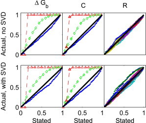
Comparison of stated and actual CIs. The x axis is the stated CI and the y axis is the observed fraction of simulations (based on 1000 simulations) in which the CI contains the true value of (left), the nonconstant elements of C (middle), and every 23rd angle for every reference pattern in R (right). In the left and middle panels, results from ordinary least squares (diamonds connected by a dashed line) and weighted least squares using the sample variance (circles connected by a dotted line) are shown along with results from weighted least squares using the shrinkage variance (points). In the middle panels, results from different matrix elements of C overlap and are essentially indistinguishable. In the right panel, the different colors denote different matrix elements of R.
Experimental results
As a demonstration of our method, we conducted and analyzed WAXS experiments on several protein-ligand systems: lysozyme and the carbohydrate (NAG)n, for , 2, and 3; galectin and the simple sugar lactose; and ADH and its cofactor, NAD+.
Lysozyme-(NAG)n
The trend in (NAG)n binding affinities estimated from WAXS with SVD preprocessing (Table 1) is consistent with the literature. Based on fluorescence measurements, the binding free energies of −2.22 kcal/mol for NAG, −4.95 kcal/mol for (NAG)2, and −7.23 kcal/mol for (NAG)3 were measured at pH 5.3 and (42). Isothermal titration calorimetry (ITC) yielded binding free energies of −5.16 kcal/mol for (NAG)2 and −7.06 for (NAG)3 in 0.1 M buffer acetate at pH 4.7 and , and also showed that (NAG)n binding is an enthalpy-driven process (43). The stronger binding seen under the conditions used here may be due to a reduced entropic penalty at lower temperature and higher protein concentration.
Table 1.
Estimated binding free energies (kcal mol−1) for the protein-ligand systems described in this work, and upper and lower bounds of the 68% CI for
| Protein | Ligand | With SVD |
Without SVD |
||||
|---|---|---|---|---|---|---|---|
| Lower | Upper | Lower | Upper | ||||
| Lysozyme | NAG | −2.98 | −3.02 | −2.94 | −7.43 | −7.54 | −7.33 |
| Lysozyme | (NAG)2 | −5.73 | −5.80 | −5.67 | −5.03 | −5.04 | −5.01 |
| Lysozyme | (NAG)3 | −12.82 | −14.31 | −11.10 | −5.14 | −5.16 | −5.12 |
| Galectin | lactose | −5.47 | −5.53 | −5.41 | −5.08 | −5.10 | −5.06 |
| ADH | NAD+ | −3.86 | −3.88 | −3.83 | −3.93 | −3.95 | −3.91 |
On the other hand, analyzing the same WAXS data without SVD preprocessing led to unreasonable results for the binding affinity of NAG and (NAG)3 (Table 1). This error indicates that although the four-species model may be a good approximation to the data, the remaining singular values in these systems are not purely random noise with a zero-mean random noise (a key assumption in the simulated data). Although SVD adds another step to the analysis, its role in filtering out less important components leads to more consistently accurate results across different systems. Henceforth, our discussion will thus refer to the multivariate curve resolution procedure with SVD unless specifically noted otherwise.
Fig. 2 and Figs. S1 and S2 in the Supporting Material summarize results for the binding of lysozyme to (NAG)n, for , 2, and 3, respectively. In panel A of all three figures, it is worth noting that the scattering intensity is substantially affected by increasing ligand concentration in the absence of protein. This effect, which is common to all our observed systems, makes it difficult, if not impossible, to determine the binding affinity from a single scattering angle. Therefore, it is essential to analyze data from multiple scattering angles.
Figure 2.
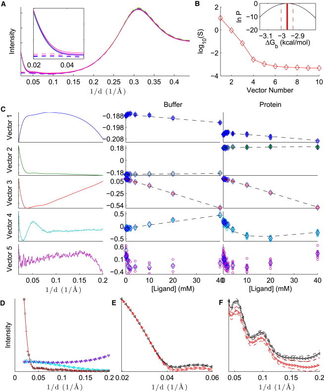
Analysis of lysozyme-NAG binding, with SVD preprocessing. (A) Average intensities for protein and ligand in buffer (solid lines), and ligand in buffer (dashed lines), in arbitrary units. The intensities increase as a function of ligand concentration. Inset: The same plot, zoomed in to the small-angle region. (B) Singular values for the first 10 basis vectors. Inset: Logarithm of the Bayesian posterior (Eq. 13) in the region where the density is within a factor of of the maximum density. (C) First five SVD basis vectors (left) and columns of V for ligand in buffer (middle column) and protein and ligand in buffer (right column). For the middle and right columns, individual measurements are denoted with circles, the mean over each concentration is indicated with diamonds, and the dashed line shows the fit of the model to the data. (D–F) Reference patterns: background (divided by 5, upward triangles), ligand (multiplied by 100, rightward triangles), apo protein (squares), and holo protein (plus signs). The figure shows an overview (D), the low-angle region of the apo and holo protein patterns on the logarithmic scale (E), and a wider-angle region of the apo and holo protein patterns on a linear scale (F). The solid line with embedded markers is the reference pattern, given the point estimate of , and the dashed lines above and below the reference patterns are the estimated upper and lower bounds, respectively, for the 68% CI. The left plot also shows other patterns that are expected to be similar to the reference patterns: the buffer, without protein or ligand (downward triangles), the difference between the highest-concentration ligand and the buffer (leftward triangles), the difference between the protein without ligand and the buffer (diamonds), and the difference between the protein at the highest ligand concentration and the buffer (x symbols). These patterns are scaled so that the sum of their absolute values matches the corresponding reference pattern (background, ligand, apo, and holo, respectively). For clarity, markers are not shown at every point.
Panel B in all three figures shows a near-exponential decline in the first four singular values. For (NAG)2 and (NAG)3, the fifth singular value is much less than the fourth and similar to the remaining singular values, suggesting that truncation at provides a good approximation to the original data set. Truncation at is also corroborated by the noisiness of the fifth basis vector and the lack of a clear trend in the corresponding coordinates D as a function of ligand concentration (bottom of panel C). For NAG, the significance of the fourth vector is less clear (the fourth is closer to the fifth singular value), but trends in panel C show that the fourth basis vector is clearly not noise, and the fifth is noisier. This supports the four-species assumption in our model.
Strictly speaking, the singular value basis vectors shown in panel C are not physically meaningful—they are merely mathematical constructs obtained by decomposition of the data matrix. Nonetheless, some clear trends are evident in the data: the first two columns of D are mostly changed by the presence or absence of protein, the third is nearly linear with ligand concentration, and the fourth has the overall shape of a binding curve (continuously increasing or decreasing until saturation is reached). The rough correspondence between coordinates in the singular value basis vector space and behavior of the concentration matrix provides evidence that the four-species model describes causes of the largest changes in scattering patterns.
Especially with NAG, the model of C fits to the data very well, and modifying by as little as 0.1 kcal/mol results in a substantially worse fit to the data. The goodness of this particular fit is summarized by the sharp Bayesian posterior in panel B. On the other hand, whereas the posteriors for NAG and (NAG)2 are fairly narrow, the posterior for (NAG)3 is broad. This is because the protein concentrations and binding affinities are high enough that for [(NAG)3]o < [M]o, any (NAG)3 added to the solution binds to the protein. At higher concentrations, the protein is saturated. This behavior is consistent with a broad range of strong binding affinities, and the log posterior below is essentially flat. In this case, it is clear that we have an upper bound rather than a complete estimate of the binding free energy. This fact may be missed with a nonBayesian analysis.
Upon binding of (NAG)n, reference patterns appear to retain the same overall shape but have shifts in intensity versus the apo patterns. This may be due to changes in solvent contrast, differences in the structural ensemble of the protein-ligand complex compared with unbound protein, or other factors that remain to be determined.
The reference patterns are also in close agreement with corresponding patterns obtained by direct subtraction: is similar to the buffer, is similar to the difference between the highest-concentration ligand and buffer, is similar to the difference between the protein and buffer, and R4 is similar to the difference between the protein with the highest concentration of ligand and the buffer. Because the reference patterns correspond to the most significant changes in the data due to changes in the concentrations of species, it is reasonable to expect that they can be approximated by simple subtractions.
Galectin-lactose
Results from the binding of galectin and lactose are summarized in Fig. 3. Although galectin is predominantly a homodimer in solution (it may also be monomeric at lower concentrations (44)), its carbohydrate-binding domains are located at opposite ends of the complex, distal to the dimerization interface (45). The WAXS data are well explained by assuming that the two binding sites are independent and applying a 1:1 binding model to the monomer, as seen by the existence of four significant singular values (Fig. 3 B), the fit of the model to D (Fig. 3 C), and the narrow posterior (Fig. 3 B, inset). The one-site model is also a good fit to ITC data (45,46). Reported binding free energies from ITC include −4.9 kcal/mol in PBS at (45), −4.7 kcal/mol in pH 7.4 PBS at (46), and −5.0 kcal/mol in pH 7.6 PBS at (47), consistent with WAXS without SVD but somewhat weaker than WAXS with SVD (Table 1). As with (NAG)n binding to lysozyme, the stronger binding of lactose to galectin observed in WAXS experiments may be explained by the fact that binding is enthalpy driven (45,46), and the conditions used here may reduce the entropic penalty.
Figure 3.
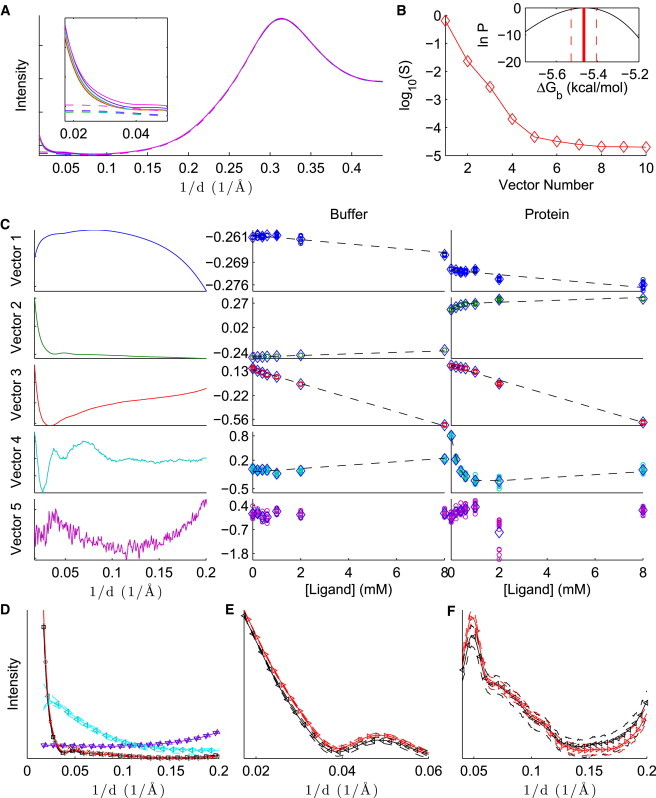
Analysis of galectin-lactose binding, with SVD preprocessing. The caption is the same as in Fig. 2.
Nesmelova et al. (46) also analyzed their data using a sequential binding model with negative cooperativity. Although ITC data were equally consistent with independent and sequential models, NMR data and molecular-dynamics simulations favored the latter. Because WAXS data are already well explained by the 1:1 binding model, as with ITC, a sequential binding model is unlikely to improve the fit to the current data set. A more complex model, however, may be necessary to explain a more detailed data set with more ligand concentrations. (Complex binding models can be considered in future work.) The insight gained by Nesmelova et al. into sequential binding highlights the importance of applying multiple biophysical techniques to study a system.
Binding of lactose to galectin leads to subtle but interpretable changes in the scattering pattern (Fig. 3 D). By applying the Guinier approximation (1), , to data between , we estimate for the apo and for the holo forms, which arguably are indistinguishable. Although this range of q is at wider angles than is typical for Guinier analysis, the observed -values are consistent with those estimated from SAXS () and small-angle neutron scattering (SANS; ) for the apo form, calculated using an indirect Fourier transform (48). Using SANS, He et al. (48) also observed a contraction to upon binding of a different ligand, N-acetyllactosamine. We do not observe such a dramatic global effect upon lactose binding. Rather, the holo scattering appears to have a slightly higher intensity relative to the apo pattern below . This shift may be due to changes in solvent contrast, as lactose may increase the solvent electron density. Between , however, the holo protein reference pattern appears slightly smoother; subtle peaks and troughs are less evident. Smoother WAXS patterns are indicative of increased diversity in the structural ensemble (12). Increased structural diversity upon lactose binding is also corroborated by NMR results indicating dampening of motion around the binding domain but increased motion elsewhere throughout the protein (46). This effect has also been observed in the related protein galectin-3 (49).
Note that the reference pattern for the holo protein is considerably different from the pattern obtained by direction subtraction (Fig. 3 D, left). Because the direct subtraction includes contributions from free ligand and free protein, it is only an approximation to the excess intensity shown in the reference patterns.
ADH-NAD+
Results from the binding of ADH and its cofactor NAD+ are summarized in Fig. S3. Although yeast ADH is a tetramer, as with galectin and lactose, we find that treating the monomers independently provides a good fit to the data (Fig. S3 C). As with the other systems studied, the magnitude of the singular values validates as a good approximation of the original scattering patterns (Fig. S3 B). The posterior is narrow (Fig. S3 B) and is consistent with spectroscopic measurements of −4.7 kcal/mol in pH 7.0, 0.1 M phosphate buffer at (50), and estimates based on kinetic rate constants ranging between −5.17 and −4.28 kcal/mol (51). As with galectin and lactose, more complex binding NAD+ models have been proposed (52); however, these will be left to future studies. Binding of NAD+ to ADH leads to shifts in the scattering pattern that may be attributed to changes in solvent contrast.
Scattering angles
In the above analyses, we used a maximum . What is the effect of increasing or decreasing this cutoff? More broadly, what is the ideal range of scattering angles to measure protein-ligand binding events?
Undoubtedly, the answer will vary from system to system and depend on many factors, including the macromolecular size, the extent to which noncovalent association modifies the structural ensemble, and whether the addition of solutes has a nonlinear effect on the solvent structure. Indeed, we observe that changing the cutoff affects the posterior of to different degrees (Fig. 4). In lysozyme-(NAG) and lysozyme-(NAG)2, changes to the low-angle intensities are not sufficiently large for us to accurately estimate the free energies solely from SAXS data. With only SAXS data, only three basis vectors are significant and the analysis procedure essentially fits to noise. On the other hand, increasing the cutoff above also leads to changes in the posterior of ; this is especially dramatic with lysozyme-NAG. The highest scattering angles can be particularly influenced by solvent structure changes that are not explained by the 1:1 binding model. As more wide-angle data are included in the analysis, a fifth, solvent-like basis vector emerges as an important factor, mixing with and sometimes overwhelming the fourth basis vector. Fortunately, for the systems studied here (and likely many other protein-ligand systems), there appears to be a plateau in around where ligand binding is detected but the data are not too strongly affected by nonlinear solvent changes. Because including more data appears to lead to narrower posteriors, a cutoff of is a reasonable choice.
Figure 4.
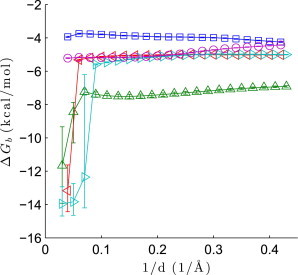
Dependence of estimates on the maximum value of , for lysozyme-NAG (upward triangles), lysozyme-(NAG)2 (leftward triangles), lysozyme-(NAG)3 (rightward triangles), galectin-lactose (circles), and ADH-NAD+ (squares). The marker is the point estimate and the error bars are the upper and lower bounds of the 68% CIs.
Discussion
In this study, we have developed and demonstrated a new way, to our knowledge, to use WAXS to study protein-ligand binding. The method provides estimates of binding free energies and, under certain assumptions about the error structure, accurate CIs. It also resolves scattering patterns indicative of different species in solution.
When we compared different variants of the method, we found that estimating the variance with a shrinkage approximation was essential. Although SVD preprocessing reduces the performance of the method with simulated data, we found it was necessary for the analysis of experimental data sets. SVD filters out high-order singular values that are not explained by the binding model.
The fact that experimental data are well described by the 1:1 binding model provides an important proof of principle that observed changes in scattering patterns are indeed due to binding events and not merely to, for example, solvent structure or contrast changes. Previously, the only available method to assess whether a scattering pattern changes because of ligand binding was to compare observed scattering pattern changes with predictions based on three-dimensional structures of apo and holo proteins (8,9).
However, the fact that a simple binding model and only four significant basis vectors describe ligand interactions with a dimeric (galectin) and a tetrameric (ADH) protein points to a current limitation of WAXS. With these multimers, partially liganded states should be observed as additional basis vectors, but the instrumental signal/noise ratio and the amount of data collected only clearly distinguish four. In other systems in which a larger number of basis vectors are observed, more complex binding models should be applied.
In addition to WAXS studies of protein-ligand binding, the described statistical analysis may be applied to other multivariate data, including data from SAXS. Although SAXS data may be inadequate for deriving the binding free energies when ligand-induced structural changes are subtle, as is the case for some of the systems described here, SAXS may allow comparable characterizations when the structural changes include alterations in the overall shape or disposition of subunits. Although this limitation may preclude many protein-ligand binding processes, related analyses may be applied to processes more readily detectable with SAXS.
Indeed, Williamson et al. (26) used a similar approach to study protein oligomerization with SAXS. A significant difference between their method and ours is that their error function is not directly associated with CIs. One benefit of their method, however, is that they considered different types of concentration models, not just simple 1:1 binding. Comparisons of more complex protein-ligand binding models, applied to data with a larger number of detected basis vectors, may be considered in future work.
With the increasing availability of x-ray solution scattering facilities at synchrotron radiation sources, and advances in robotic technology for loading and analyzing samples, we foresee further applications of the described approach, such as for quantitative moderate-throughput screening of small-molecule fragments. Our method may also inspire progress in Bayesian chemometrics (53).
Acknowledgments
We thank David Gore, Robert F. Fischetti, and Suneeta Mandava for assistance with data collection at BioCAT. We thank Peter McCullagh for statistical consulting and John Chodera for helpful comments on the manuscript.
This work was supported by a Director’s Postdoctoral Fellowship to D.D.L.M. and research grants from the National Institutes of Health (R01GM-085648) and the National Science Foundation (1158340) to L.M. BioCAT is a research center (RR-08630) supported by the National Institutes of Health. The use of the Advanced Photon Source, an Office of Science user facility operated for the U.S. Department of Energy Office of Science by Argonne National Laboratory, was supported by the U.S. Department of Energy.
The manuscript was created in part by UChicago Argonne, LLC, Operator of Argonne National Laboratory (Argonne), a U.S. Department of Energy Office of Science laboratory. Argonne National Laboratory and the Advanced Photon Source are operated under contract No. DE-AC02-06CH11357. The U.S. Government retains for itself, and others acting on its behalf, a paid-up nonexclusive, irrevocable worldwide license in said article to reproduce, prepare derivative works, distribute copies to the public, and perform publicly and display publicly, by or on behalf of the government.
Footnotes
David D. L. Minh’s present address is Department of Chemistry, Duke University, Durham, North Carolina.
Supporting Material
References
- 1.Glatter O., Kratky O. Academic Press; London: 1982. Small Angle X-Ray Scattering. [Google Scholar]
- 2.Semenyuk A.V., Svergun D.I. GNOM—a program package for small-angle scattering data-processing. J. Appl. Cryst. 1991;24:537–540. [Google Scholar]
- 3.Lipfert J., Doniach S. Small-angle X-ray scattering from RNA, proteins, and protein complexes. Annu. Rev. Biophys. Biomol. Struct. 2007;36:307–327. doi: 10.1146/annurev.biophys.36.040306.132655. [DOI] [PubMed] [Google Scholar]
- 4.Svergun D.I. Small-angle X-ray and neutron scattering as a tool for structural systems biology. Biol. Chem. 2010;391:737–743. doi: 10.1515/BC.2010.093. [DOI] [PubMed] [Google Scholar]
- 5.Mertens H.D.T., Svergun D.I. Structural characterization of proteins and complexes using small-angle X-ray solution scattering. J. Struct. Biol. 2010;172:128–141. doi: 10.1016/j.jsb.2010.06.012. [DOI] [PubMed] [Google Scholar]
- 6.Makowski L., Rodi D.J., Fischetti R.F. Characterization of protein fold by wide-angle X-ray solution scattering. J. Mol. Biol. 2008;383:731–744. doi: 10.1016/j.jmb.2008.08.038. [DOI] [PubMed] [Google Scholar]
- 7.Makowski L., Rodi D.J., Fischetti R.F. Molecular crowding inhibits intramolecular breathing motions in proteins. J. Mol. Biol. 2008;375:529–546. doi: 10.1016/j.jmb.2007.07.075. [DOI] [PMC free article] [PubMed] [Google Scholar]
- 8.Fischetti R.F., Rodi D.J., Makowski L. Wide-angle X-ray solution scattering as a probe of ligand-induced conformational changes in proteins. Chem. Biol. 2004;11:1431–1443. doi: 10.1016/j.chembiol.2004.08.013. [DOI] [PubMed] [Google Scholar]
- 9.Rodi D.J., Mandava S., Fischetti R.F. Detection of functional ligand-binding events using synchrotron x-ray scattering. J. Biomol. Screen. 2007;12:994–998. doi: 10.1177/1087057107306104. [DOI] [PubMed] [Google Scholar]
- 10.Cho H.S., Dashdorj N., Anfinrud P. Protein structural dynamics in solution unveiled via 100-ps time-resolved x-ray scattering. Proc. Natl. Acad. Sci. USA. 2010;107:7281–7286. doi: 10.1073/pnas.1002951107. [DOI] [PMC free article] [PubMed] [Google Scholar]
- 11.Makowski L., Bardhan J., Fischetti R.F. WAXS studies of the structural diversity of hemoglobin in solution. J. Mol. Biol. 2011;408:909–921. doi: 10.1016/j.jmb.2011.02.062. [DOI] [PMC free article] [PubMed] [Google Scholar]
- 12.Makowski L., Gore D., Fischetti R.F. X-ray solution scattering studies of the structural diversity intrinsic to protein ensembles. Biopolymers. 2011;95:531–542. doi: 10.1002/bip.21631. [DOI] [PMC free article] [PubMed] [Google Scholar]
- 13.Zuo X.B., Tiede D.M. Resolving conflicting crystallographic and NMR models for solution-state DNA with solution X-ray diffraction. J. Am. Chem. Soc. 2005;127:16–17. doi: 10.1021/ja044533+. [DOI] [PubMed] [Google Scholar]
- 14.Zuo X.B., Cui G.L., Tiede D.M. X-ray diffraction “fingerprinting” of DNA structure in solution for quantitative evaluation of molecular dynamics simulation. Proc. Natl. Acad. Sci. USA. 2006;103:3534–3539. doi: 10.1073/pnas.0600022103. [DOI] [PMC free article] [PubMed] [Google Scholar]
- 15.Zuo X.B., Wang J.B., Wang Y.X. Global molecular structure and interfaces: refining an RNA:RNA complex structure using solution X-ray scattering data. J. Am. Chem. Soc. 2008;130:3292–3293. doi: 10.1021/ja7114508. [DOI] [PubMed] [Google Scholar]
- 16.Sivaramakrishnan S., Sung J., Spudich J.A. Combining single-molecule optical trapping and small-angle x-ray scattering measurements to compute the persistence length of a protein ER/K alpha-helix. Biophys. J. 2009;97:2993–2999. doi: 10.1016/j.bpj.2009.09.009. [DOI] [PMC free article] [PubMed] [Google Scholar]
- 17.Ali M., Lipfert J., Doniach S. The ligand-free state of the TPP riboswitch: a partially folded RNA structure. J. Mol. Biol. 2010;396:153–165. doi: 10.1016/j.jmb.2009.11.030. [DOI] [PMC free article] [PubMed] [Google Scholar]
- 18.Wang Y.X., Zuo X.B., Butcher S.E. Rapid global structure determination of large RNA and RNA complexes using NMR and small-angle X-ray scattering. Methods. 2010;52:180–191. doi: 10.1016/j.ymeth.2010.06.009. [DOI] [PMC free article] [PubMed] [Google Scholar]
- 19.Yang S.C., Parisien M., Roux B. RNA structure determination using SAXS data. J. Phys. Chem. B. 2010;114:10039–10048. doi: 10.1021/jp1057308. [DOI] [PMC free article] [PubMed] [Google Scholar]
- 20.Boura E., Rózycki B., Hurley J.H. Solution structure of the ESCRT-I complex by small-angle X-ray scattering, EPR, and FRET spectroscopy. Proc. Natl. Acad. Sci. USA. 2011;108:9437–9442. doi: 10.1073/pnas.1101763108. [DOI] [PMC free article] [PubMed] [Google Scholar]
- 21.Różycki B., Kim Y.C., Hummer G. SAXS ensemble refinement of ESCRT-III CHMP3 conformational transitions. Structure. 2011;19:109–116. doi: 10.1016/j.str.2010.10.006. [DOI] [PMC free article] [PubMed] [Google Scholar]
- 22.Jaumot J., Vives M., Gargallo R. Application of multivariate resolution methods to the study of biochemical and biophysical processes. Anal. Biochem. 2004;327:1–13. doi: 10.1016/j.ab.2003.12.028. [DOI] [PubMed] [Google Scholar]
- 23.Yang S.C., Blachowicz L., Roux B. Multidomain assembled states of Hck tyrosine kinase in solution. Proc. Natl. Acad. Sci. USA. 2010;107:15757–15762. doi: 10.1073/pnas.1004569107. [DOI] [PMC free article] [PubMed] [Google Scholar]
- 24.Chen L.L., Wildegger G., Doniach S. Kinetics of lysozyme refolding: structural characterization of a non-specifically collapsed state using time-resolved X-ray scattering. J. Mol. Biol. 1998;276:225–237. doi: 10.1006/jmbi.1997.1514. [DOI] [PubMed] [Google Scholar]
- 25.Segel D.J., Bachmann A., Kiefhaber T. Characterization of transient intermediates in lysozyme folding with time-resolved small-angle X-ray scattering. J. Mol. Biol. 1999;288:489–499. doi: 10.1006/jmbi.1999.2703. [DOI] [PubMed] [Google Scholar]
- 26.Williamson T.E., Craig B.A., Friedman A.M. Analysis of self-associating proteins by singular value decomposition of solution scattering data. Biophys. J. 2008;94:4906–4923. doi: 10.1529/biophysj.107.113167. [DOI] [PMC free article] [PubMed] [Google Scholar]
- 27.Blobel J., Bernadó P., Pons M. Low-resolution structures of transient protein-protein complexes using small-angle X-ray scattering. J. Am. Chem. Soc. 2009;131:4378–4386. doi: 10.1021/ja808490b. [DOI] [PubMed] [Google Scholar]
- 28.Chen L.L., Hodgson K.O., Doniach S. A lysozyme folding intermediate revealed by solution X-ray scattering. J. Mol. Biol. 1996;261:658–671. doi: 10.1006/jmbi.1996.0491. [DOI] [PubMed] [Google Scholar]
- 29.Segel D.J., Fink A.L., Doniach S. Protein denaturation: a small-angle X-ray scattering study of the ensemble of unfolded states of cytochrome c. Biochemistry. 1998;37:12443–12451. doi: 10.1021/bi980535t. [DOI] [PubMed] [Google Scholar]
- 30.Lipfert J., Columbus L., Doniach S. Analysis of small-angle X-ray scattering data of protein-detergent complexes by singular value decomposition. J. Appl. Cryst. 2007;40:S235–S239. [Google Scholar]
- 31.Stols L., Gu M., Donnelly M.I. A new vector for high-throughput, ligation-independent cloning encoding a tobacco etch virus protease cleavage site. Protein Expr. Purif. 2002;25:8–15. doi: 10.1006/prep.2001.1603. [DOI] [PubMed] [Google Scholar]
- 32.Gasteiger E., Hoogland C., Bairoch A. Protein identification and analysis tools on the ExPASy Server. In: Walker J.M., editor. In The Proteomics Protocols Handbook. Humana Press; Totowa, NJ: 2005. pp. 571–607. [Google Scholar]
- 33.Fischetti R., Stepanov S., Bunker G.B. The BioCAT undulator beamline 18ID: a facility for biological non-crystalline diffraction and X-ray absorption spectroscopy at the Advanced Photon Source. J. Synchrotron Radiat. 2004;11:399–405. doi: 10.1107/S0909049504016760. [DOI] [PubMed] [Google Scholar]
- 34.Fischetti R.F., Rodi D.J., Makowski L. High-resolution wide-angle X-ray scattering of protein solutions: effect of beam dose on protein integrity. J. Synchrotron Radiat. 2003;10:398–404. doi: 10.1107/s0909049503016583. [DOI] [PubMed] [Google Scholar]
- 35.Hammersley A.P., Svensson S.O., Häusermann D. Two-dimensional detector software: from real detector to idealised image or two-theta scan. High Press. Res. 1996;14:235–248. [Google Scholar]
- 36.Hammersley A. ESRF; Grenoble, France: 1997. FIT2D: an introduction and overview. Technical Report ESRF97HA02T. [Google Scholar]
- 37.Cohn E.J., Edsall J.T. Reinhold; New York: 1943. Proteins, Amino Acids and Peptides as Ions and Dipolar Ions. [Google Scholar]
- 38.Park S., Bardhan J.P., Makowski L. Simulated x-ray scattering of protein solutions using explicit-solvent models. J. Chem. Phys. 2009;130:134114. doi: 10.1063/1.3099611. [DOI] [PMC free article] [PubMed] [Google Scholar]
- 39.von Neumann J. Various techniques used in connection with random digits. Monte Carlo methods. Nat. Bur. Standards AMS. 1951;12:36–38. [Google Scholar]
- 40.Henry E.R., Hofrichter J. Singular value decomposition—application to analysis of experimental data. Methods Enzymol. 1992;210:129–192. [Google Scholar]
- 41.Hendler R.W., Shrager R.I. Deconvolutions based on singular value decomposition and the pseudoinverse: a guide for beginners. J. Biochem. Biophys. Methods. 1994;28:1–33. doi: 10.1016/0165-022x(94)90061-2. [DOI] [PubMed] [Google Scholar]
- 42.Banerjee S.K., Rupley J.A. Temperature and pH dependence of the binding of oligosaccharides to lysozyme. J. Biol. Chem. 1973;248:2117–2124. [PubMed] [Google Scholar]
- 43.García-Hernández E., Zubillaga R.A., Costas M. Structural energetics of protein-carbohydrate interactions: insights derived from the study of lysozyme binding to its natural saccharide inhibitors. Protein Sci. 2003;12:135–142. doi: 10.1110/ps.0222503. [DOI] [PMC free article] [PubMed] [Google Scholar]
- 44.Salomonsson E., Larumbe A., Leffler H. Monovalent interactions of galectin-1. Biochemistry. 2010;49:9518–9532. doi: 10.1021/bi1009584. [DOI] [PubMed] [Google Scholar]
- 45.López-Lucendo M.F., Solís D., Romero A. Growth-regulatory human galectin-1: crystallographic characterisation of the structural changes induced by single-site mutations and their impact on the thermodynamics of ligand binding. J. Mol. Biol. 2004;343:957–970. doi: 10.1016/j.jmb.2004.08.078. [DOI] [PubMed] [Google Scholar]
- 46.Nesmelova I.V., Ermakova E., Mayo K.H. Lactose binding to galectin-1 modulates structural dynamics, increases conformational entropy, and occurs with apparent negative cooperativity. J. Mol. Biol. 2010;397:1209–1230. doi: 10.1016/j.jmb.2010.02.033. [DOI] [PubMed] [Google Scholar]
- 47.Meynier C., Feracci M., Roche P. NMR and MD investigations of human galectin-1/oligosaccharide complexes. Biophys. J. 2009;97:3168–3177. doi: 10.1016/j.bpj.2009.09.026. [DOI] [PMC free article] [PubMed] [Google Scholar]
- 48.He L.Z., André S., Gabius H.J. Detection of ligand- and solvent-induced shape alterations of cell-growth-regulatory human lectin galectin-1 in solution by small angle neutron and x-ray scattering. Biophys. J. 2003;85:511–524. doi: 10.1016/S0006-3495(03)74496-8. [DOI] [PMC free article] [PubMed] [Google Scholar]
- 49.Diehl C., Engström O., Akke M. Protein flexibility and conformational entropy in ligand design targeting the carbohydrate recognition domain of galectin-3. J. Am. Chem. Soc. 2010;132:14577–14589. doi: 10.1021/ja105852y. [DOI] [PMC free article] [PubMed] [Google Scholar]
- 50.Karlović D., Amiguet P., Luisi P.L. Spectroscopic investigation of binary and ternary coenzyme complexes of yeast alcohol dehydrogenase. Eur. J. Biochem. 1976;66:277–284. doi: 10.1111/j.1432-1033.1976.tb10517.x. [DOI] [PubMed] [Google Scholar]
- 51.Leskovac V., Trivic S., Kandrac J. Binding of coenzymes to yeast alcohol dehydrogenase. J. Serb. Chem. Soc. 2010;75:185–194. [Google Scholar]
- 52.Leskovac V., Trivić S., Pericin D. The three zinc-containing alcohol dehydrogenases from baker’s yeast, Saccharomyces cerevisiae. FEMS Yeast Res. 2002;2:481–494. doi: 10.1111/j.1567-1364.2002.tb00116.x. [DOI] [PubMed] [Google Scholar]
- 53.Chen H., Bakshi B.R., Goel P.K. Toward Bayesian chemometrics—a tutorial on some recent advances. Anal. Chim. Acta. 2007;602:1–16. doi: 10.1016/j.aca.2007.08.044. [DOI] [PubMed] [Google Scholar]
Associated Data
This section collects any data citations, data availability statements, or supplementary materials included in this article.