A guide to appropriate use of Correlation coefficient in medical research

Abstract

Correlation is a statistical method used to assess a possible linear association between two continuous variables. It is simple both to calculate and to interpret. However, misuse of correlation is so common among researchers that some statisticians have wished that the method had never been devised at all. The aim of this article is to provide a guide to appropriate use of correlation in medical research and to highlight some misuse. Examples of the applications of the correlation coefficient have been provided using data from statistical simulations as well as real data. Rule of thumb for interpreting size of a correlation coefficient has been provided.

Definitions of correlation and clarifications

The term correlation is sometimes used loosely in verbal communication. Among scientific colleagues, the term correlation is used to refer to an association, connection, or any form of relationship, link or correspondence. This broad colloquial definition sometimes leads to misuse of the statistical term “correlation” among scientists in research. Misuse of correlation is so common that some statisticians have wished that the method had never been devised.¹

Webster's Online Dictionary defines correlation as a reciprocal relation between two or more things; a statistic representing how closely two variables co-vary; it can vary from −1 (perfect negative correlation) through 0 (no correlation) to +1 (perfect positive correlation).²

In statistical terms, correlation is a method of assessing a possible two-way linear association between two continuous variables.¹ Correlation is measured by a statistic called the correlation coefficient, which represents the strength of the putative linear association between the variables in question. It is a dimensionless quantity that takes a value in the range −1 to +1³. A correlation coefficient of zero indicates that no linear relationship exists between two continuous variables, and a correlation coefficient of −1 or +1 indicates a perfect linear relationship. The strength of relationship can be anywhere between −1 and +1. The stronger the correlation, the closer the correlation coefficient comes to ±1. If the coefficient is a positive number, the variables are directly related (i.e., as the value of one variable goes up, the value of the other also tends to do so). If, on the other hand, the coefficient is a negative number, the variables are inversely related (i.e., as the value of one variable goes up, the value of the other tends to go down).³ Any other form of relationship between two continuous variables that is not linear is not correlation in statistical terms. To emphasise this point, a mathematical relationship does not necessarily mean that there is correlation. For example, consider the equation y=2×2. In statistical terms, it is inappropriate to say that there is correlation between x and y. This is so because, although there is a relationship, the relationship is not linear over this range of the specified values of x. It is possible to predict y exactly for each value of x in the given range, but correlation is neither −1 nor +1. Hence, it would be inconsistent with the definition of correlation and it cannot therefore be said that x is correlated with y.

Types of correlation coefficients⁴

There are two main types of correlation coefficients: Pearson's product moment correlation coefficient and Spearman's rank correlation coefficient. The correct usage of correlation coefficient type depends on the types of variables being studied. We will focus on these two correlation types; other types are based on these and are often used when multiple variables are being considered.

Pearson's product moment correlation coefficient

Pearson's product moment correlation coefficient is denoted as ϱ for a population parameter and as r for a sample statistic. It is used when both variables being studied are normally distributed. This coefficient is affected by extreme values, which may exaggerate or dampen the strength of relationship, and is therefore inappropriate when either or both variables are not normally distributed. For a correlation between variables x and y, the formula for calculating the sample Pearson's correlation coefficient is given by³

$$r=\frac{{\displaystyle \sum _{i=1}^n(x_i-x)(y_i-y)}}{\sqrt{\left[{\displaystyle \sum _{i=1}^n{(x_i-\overline{x})}^2}\right]\left[{\displaystyle \sum _{i=1}^n{(y_i-\overline{y})}^2}\right]}}$$

where xi and yi are the values of x and y for the ith individual.

Spearman's rank correlation coefficient

Spearman's rank correlation coefficient is denoted as ϱs for a population parameter and as rs for a sample statistic. It is appropriate when one or both variables are skewed or ordinal¹ and is robust when extreme values are present. For a correlation between variables x and y, the formula for calculating the sample Spearman's correlation coefficient is given by

$$r_s=1-\frac{6{\displaystyle \sum _{i=1}^n{d}_i^2}}{n(n^2-1)}\text{\hspace{0.17em}where di is the difference in ranks for x and y}$$

The distinction between Pearson's and Spearman's correlation coefficients in applications will be discussed using examples below.

Relationship between correlation coefficient and scatterplots using statistical simulations

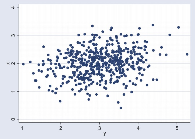
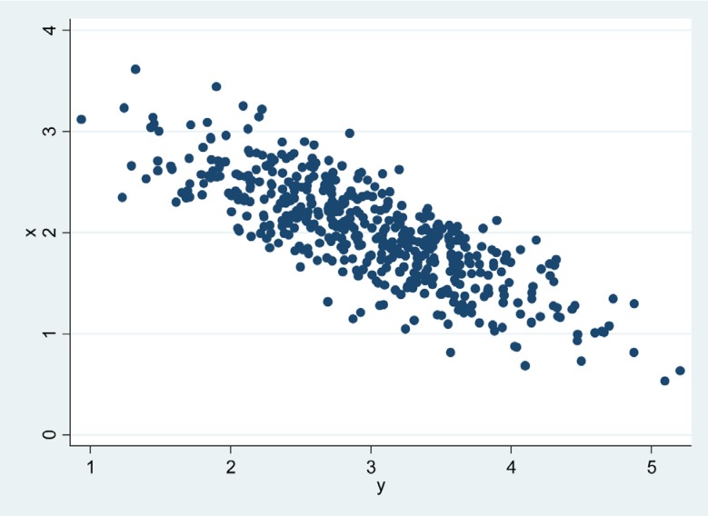
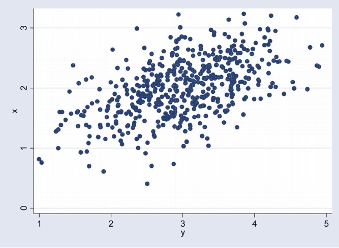
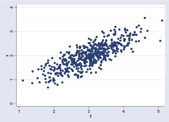
The data depicted in figures 1–4 were simulated from a bivariate normal distribution of 500 observations with means 2 and 3 for the variables x and y respectively. The standard deviations were 0.5 for x and 0.7 for y. Scatter plots were generated for the correlations 0.2, 0.5, 0.8 and −0.8.

Fig. 1.

Scatterplot of x and y: Pearson's correlation=0.2

Fig. 4.

Scatterplot of x and y: Pearson's correlation=−0.80

In Fig. 1, the scatter plot shows some linear trend but the trend is not as clear as that of Fig. 2. The trend in Fig. 3 is clearly seen and the points are not as scattered as those of Figs. 1 and 2. That is, the higher the correlation in either direction (positive or negative), the more linear the association between two variables and the more obvious the trend in a scatter plot. For Figures 3 and 4, the strength of linear relationship is the same for the variables in question but the direction is different. In Figure 3, the values of y increase as the values of x increase while in figure 4 the values of y decrease as the values of x increase.

Fig. 2.

Scatterplot of x and y: Pearson's correlation=0.50

Fig. 3.

Scatterplot of x and y: Pearson's correlation=0.80

Practical use of correlation coefficient

Simple application of the correlation coefficient can be exemplified using data from a sample of 780 women attending their first antenatal clinic (ANC) visits. We can expect a positive linear relationship between maternal age in years and parity because parity cannot decrease with age, but we cannot predict the strength of this relationship. The task is one of quantifying the strength of the association. That is, we are interested in the strength of relationship between the two variables rather than direction since direction is obvious in this case. Maternal age is continuous and usually skewed while parity is ordinal and skewed. With these scales of measurement for the data, the appropriate correlation coefficient to use is Spearman's. The Spearman's coefficient is 0.84 for this data. In this case, maternal age is strongly correlated with parity, i.e. has a high positive correlation (Table 1). The Pearson's correlation coefficient for these variables is 0.80. In this case the two correlation coefficients are similar and lead to the same conclusion, however in some cases the two may be very different leading to different statistical conclusions. For example, in the same group of women the spearman's correlation between haemoglobin level and parity is 0.3 while the Pearson's correlation is 0.2. In this case the two coefficients may lead to different statistical inference. For example, a correlation coefficient of 0.2 is considered to be negligible correlation while a correlation coefficient of 0.3 is considered as low positive correlation (Table 1), so it would be important to use the most appropriate one. The most appropriate coefficient in this case is the Spearman's because parity is skewed.

Table 1.

Rule of Thumb for Interpreting the Size of a Correlation Coefficient⁴

Size of Correlation	Interpretation
.90 to 1.00 (−.90 to −1.00)	Very high positive (negative) correlation
.70 to .90 (−.70 to −.90)	High positive (negative) correlation
.50 to .70 (−.50 to −.70)	Moderate positive (negative) correlation
.30 to .50 (−.30 to −.50)	Low positive (negative) correlation
.00 to .30 (.00 to −.30)	negligible correlation

In another dataset of 251 adult women, age and weight were log-transformed. The reason for transforming was to make the variables normally distributed so that we can use Pearson's correlation coefficient. Then we analysed the data for a linear association between log of age (agelog) and log of weight (wlog). Both variables are approximately normally distributed on the log scale. In this case Pearson's correlation coefficient is more appropriate. The coefficient is 0.184. This shows that there is negligible correlation between the age and weight on the log scale (Table 1).

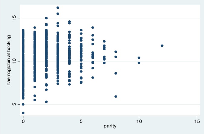
In Fig. 5 the pattern changes at the higher values of parity. Table 2 shows how Spearman's and Pearson's correlation coefficients change when seven patients having higher values of parity have been excluded. When the seven higher parity values are excluded, Pearson's correlation coefficient changes substantially compared to Spearman's correlation coefficient. Although the difference in the Pearson Correlation coefficient before and after excluding outliers is not statistically significant, the interpretation may be different. The correlation coefficient of 0.2 before excluding outliers is considered as negligible correlation while 0.3 after excluding outliers may be interpreted as weak positive correlation (Table 1). The interpretation for the Spearman's correlation remains the same before and after excluding outliers with a correlation coefficient of 0.3. The difference in the change between Spearman's and Pearson's coefficients when outliers are excluded raises an important point in choosing the appropriate statistic. Non-normally distributed data may include outlier values that necessitate usage of Spearman's correlation coefficient.

Fig. 5.

A scatter plot of haemoglobin against parity for 783 women attending ANC visit number 1

Table 2.

Spearman's and Pearson's Correlation coefficients for haemoglobin against parity

Statistic	Extreme values included		Extreme values removed
	n	r	n	r
Spearman's	783	0.3	776	0.3
Pearson's	783	0.2	776	0.3

Conclusion

In summary, correlation coefficients are used to assess the strength and direction of the linear relationships between pairs of variables. When both variables are normally distributed use Pearson's correlation coefficient, otherwise use Spearman's correlation coefficient. Spearman's correlation coefficient is more robust to outliers than is Pearson's correlation coefficient. Correlation coefficients do not communicate information about whether one variable moves in response to another. There is no attempt to establish one variable as dependent and the other as independent. Thus, relationships identified using correlation coefficients should be interpreted for what they are: associations, not causal relationships.⁵ Correlation must not be used to assess agreement between methods. Agreement between methods should be assessed using Bland-Altman plots⁶.

References

- 1.Altman DG. Practical Statistics for Medical Research. Chapman & Hall/CRC; [Google Scholar]
- 2.Webster's Online Dictionary. [Google Scholar]
- 3.Swinscow TDV. In: Statistics at square one. Nineth Edition. Campbell M J, editor. University of Southampton; Copyright BMJ Publishing Group 1997. [Google Scholar]
- 4.Hinkle DE, Wiersma W, Jurs SG. Applied Statistics for the Behavioral Sciences. 5th ed. Boston: Houghton Mifflin; 2003. [Google Scholar]
- 5.Clarke GM, Cooke D. A basic course in Statistics. 3rd ed [Google Scholar]
- 6.Altman DG, Bland JM. Measurement in Medicine: The Analysis of Method Comparison Studies. The Statistician. 1983;32:307–317. [Google Scholar]