

Abstract

Metabolomics is likely an ideal tool to assess tobacco smoke exposure and the impact of cigarette smoke on human exposure and health. To assess reproducibility and feasibility of this by UPLC–QTOF-MS, three experiments were designed for the assessment of smokers’ blood. Experiment I was an analysis of 8 smokers with 8 replicates. Experiment II was an analysis of 62 pooled quality control (QC) samples from 7 nonsmokers’ plasma placed as every tenth sample among a study of 613 samples from 160 smokers. Finally, to examine the feasibility of metabolomic study in assessing smoke exposure, Experiment III consisted of 9 smokers and 10 nonsmokers’ serum to evaluate differences in their global metabolome. There was minimal measurement and sample preparation variation in all experiments, although some caution is needed when analyzing specific parts of the chromatogram. When assessing QC samples in the large scale study, QC clustering indicated high stability, reproducibility, and consistency. Finally, in addition to the identification of nicotine metabolites as expected, there was a characteristic profile distinguishing smokers from nonsmokers. Metabolites selected from putative identifications were verified by MS/MS, showing the potential to identify metabolic phenotypes and new metabolites relating to cigarette smoke exposure and toxicity.
Keywords: metabolomics, metabolism, nicotine, validation, carcinogens
Introduction
Tobacco smoking is a major cause of morbidity and mortality in developed countries.1 There are more than 4500 identified chemicals2 and over 60 potential or probable human carcinogens in cigarette smoke.2 The complex mixture of cigarette smoke has been classified by IARC (The International Agency for Research on Cancer) as a Group 1 known human carcinogen.3 The Institute of Medicine (IOM) in 2000, at the request of the Food and Drug Administration (FDA), considered whether harm reduction approaches through reducing toxin exposures in smoke via modified-risk tobacco products (MRTPs) could feasibly enhance tobacco control for smokers who will not or could not quit.4 They concluded that such an approach was feasible. Recently, the FDA has been given legislative authority over tobacco products, including the ability to establish performance standards (e.g., regulating the amount of carcinogen emissions and exposure to smokers through product design changes) and evaluating manufacturers’ health claims of MRTPs.5 In the last several years, there has been a renewed interest by the tobacco companies to manufacture these.6 While tobacco product design changes developed by the manufacturers or mandated by the FDA can be screened in the laboratory for changes in smoke chemical constituents and toxicology,7 ultimately the impact of such changes must be evaluated in humans using biomarkers. However, there are only a limited number of biomarkers that assess exposure, and none that have been sufficiently validated for lung cancer risk.8 Given the wide variety of tobacco toxicants, a broad range of biomarkers needs to be developed and validated to assess the impact of cigarette design changes on human exposure and health.
The best available cigarette smoke biomarkers are chemically specific, reflecting only a narrow range of known toxicants. These target polycyclic aromatic hydrocarbons (e.g., benzo(a)pyrene), tobacco-specific nitrosamines (e.g., NNN, NNK), aromatic amines, and volatile hydrocarbons (e.g., benzene, 1,3-butadiene and acrolein).9−11 Among these, polycyclic aromatic hydrocarbons (PAHs) and tobacco-specific nitrosamines (TSNAs) are considered the major causative agents in cigarette smoke contributing to lung cancer,12−14 and for cancer risk overall.15 1,3-Butadiene is a potent lung carcinogen in experimental animals.15 Acrolein is a suspected human carcinogen and carries the highest level of risk for respiratory effects in experimental animals,15 while benzene is a known human leukemogen.16
Metabolomics is an ‘omics technology that provides a simultaneous assessment of numerous molecules (i.e., the metabolome) allowing for the quantification of individual metabolites and the identification of a phenotypic profile for clusters of metabolites.17−19 It provides information about metabolites from exogenous toxin exposures and those from cellular endogenous pathways as a result of the toxic exposures.17 In contrast to currently available smoke exposure biomarkers that are mostly chemically specific,13 metabolomics can provide information allows for broader phenotype assessments incorporating profiles within and across disease pathways. Separately, metabolomics provide phenotypic information about the cell’s environment and mechanistic pathways that genomics and transcriptomics do not.20,21 Metabolomics is becoming an important component of systems biology, especially in determining the global metabolic profile by detecting thousands of small and large molecules in various media ranging from cell cultures to human biological fluids such as urine, saliva, and blood.18,22−25 More and more modern instrumentations and technologies are emerging for the metabolomics research, such as gas chromatography–mass spectrometry (GC–MS), liquid chromatography–mass spectrometry (LC–MS), high-performance liquid chromatography coupled with electrochemical coulometric array (LCECA), and nuclear magnetic resonance (NMR)-based study.26 Each platform has its specific strengths and weaknesses. For example, GC–MS has great separation efficiency and resolution but analyzes only the volatile metabolic compounds;27 LCECA has great reproducibility and sensitivity but is low-throughput and provides only limited chemical structure information;19,28,29 NMR is a fast and reliable nondestructive detector but has poor resolving power and poor sensitivity requiring larger amount of analyte compared to mass spectrometry.19,29,30 LC–MS is an important tool with great flexibility in metabolomics compared to the other methods.31 It is often used to identify the low-abundance metabolites for a targeted study or to obtain the largest metabolomics profile for a global approach. With the development of Ultrahigh Pressure Liquid Chromatography (UPLC), better chromatographic resolution and peak capacity compared to HPLC is achieved, and therefore it has become the platform of choice in our study.19,32
There has been a great increase in the research of metabolomics, and a number of studies have shown the utility in assessing human disease risk.33−35 However, while some studies show the utility in urine samples,36−39 little has been shown to validate the reproducibility of global metabolomics profile using LC–MS on human blood samples.40 Thus, this study assesses Ultra Performance Liquid Chromatography coupled to Quadrupole with Time-of-Flight Mass Spectrometry (UPLC–QTOF-MS) method for use in metabolomics and applies the procedure to human samples from smokers and nonsmokers.
Materials and Methods
Reagents and Chemicals
All reagents and solvents were of HPLC grade. 4-nitrobenzoic acid (4-NBA), debrisoquine (as debrisoquine sulfate), cotinine, (±)-nicotine, 1,11-undecanedicarboxylic acid and 3-hydroxycoumarin were purchased from Sigma-Aldrich (St. Louis, MO); pseudooxynicotine, 3-hydroxycotinine, and cotinine N-oxide were purchased from Toronto Research Chemicals (North York, ON, Canada); acetonitrile (ACN) and water were purchased from Fisher Optima grade (Fisher Scientific, Waltham, MA).
Experimental Design
Three experiments were conducted. In Experiment I, in order to test the variations of UPLC–QTOF-MS assay, eight smokers’ plasma were split into two aliquots (5 μL), and one aliquot was sampled consecutively 5 times, immediately followed by the second aliquot sampled three times. A water blank was sampled between each of the subjects. The eight subjects were sampled consecutively, followed by a repeat of the experiment for the first two subjects. Replicate comparison analysis is indicated below.
Experiment II takes advantage of a quality control procedure used for ensuring assay consistency during the course of a large sample set analysis. Here, a pooled sample from 7 nonsmoker subjects undergoing therapeutic phlebotomy were placed as every tenth sample among a sample set of 613 independent samples from 160 smokers; 62 injections of the pooled control were analyzed. Replicate comparison analysis is indicated below.
Experiment III was intended to determine if there was a metabolomic result difference between smokers and nonsmokers. There were nine smokers and ten nonsmokers; the latter recruited from a three-arm study validating biomarkers in smokers, former smokers, and nonsmokers.
Subjects
Smokers: Blood samples were obtained from 160 cross-sectional study of smokers intended to characterize cigarette smoke exposure and the development and validation of biomarkers. These individuals were healthy and had no history of cancer. As an eligibility criterion, they had a stable smoking pattern for at least 6 months of 10 cigarettes per day or more. There were 613 samples from these subjects that were analyzed in a single session. Interspersed with these samples were replicates as indicated in Experiment II. Non-Smokers: Two groups of nonsmokers were utilized. The samples in the first group, used for the laboratory validation studies for Experiment II, were nonsmokers who were undergoing therapeutic phlebotomy for hemachromatosis or myeloproliferative diseases. The former had low iron levels and both groups had stable disease. Their plasma was pooled and aliquots were interspersed with the smokers’ samples in every tenth aliquot. The second group, used to assess metabolomic differences between smokers and nonsmokers for Experiment III, used nonsmokers from a study of biomarker validation in smokers, former smokers, and nonsmokers from the Tobacco Product Assessment Consortium (TobPRAC). These were healthy persons who smoked less than 100 cigarettes in their lifetime and recruited by IRB-approved local media.
Demographics of all the participants are listed in Supplementary Tables 1 to 3 in the Supporting Information. Blood was collected as serum or plasma (heparin green top tubes) as indicated.
UPLC–QTOF-MS Analysis
Sample aliquots were mixed with 195 μL of 66% ACN containing the internal standards debrisoquine and 4-NBA. The samples were centrifuged at 16000× g for 10 min at 4 °C to remove particulates and precipitated proteins. One-hundred fifty microliters of the supernatant was then transferred into an autosampler vial, followed by UPLC–QTOF-MS analysis. Samples were injected onto a reverse-phase 50 × 2.1 mm ACQUITY 1.7-μm C18 column (Waters, Milford, MA) using an ACQUITY UPLC system (Waters, Milford, MA) with a gradient mobile phase consisting of 2% ACN in water containing 0.1% formic acid (A) and 2% water in ACN containing 0.1% formic acid (B). Each sample was resolved for 10 min at a flow rate of 0.5 mL/min. The gradient consisted of 100% A for 0.5 min then a ramp of curve 6 to 60% B from 0.5 to 4.0 min, then a ramp of curve 6 to 100% B from 4.0 to 8.0 min, hold at 100% B until 9.0 min, then a ramp of curve 6 to 100% A from 9.0 to 9.2 min, followed by a hold at 100% A until 10 min. The column eluent was introduced directly into the mass spectrometer by electrospray. Mass spectrometry was performed on a Q-TOF Premier (Waters, Milford, MA) operating in either negative-ion (ESI−) or positive-ion (ESI+) electrospray ionization mode with a capillary voltage of 3200 V and a sampling cone voltage of 20 V in negative mode and 35 V in positive mode. The desolvation gas flow was set to 800 L/h and the temperature was set to 350 °C. The cone gas flow was 25 L/h, and the source temperature was 120 °C. Accurate mass was maintained by introduction of LockSpray interface of sulfadimethoxine (311.0814 [M + H]+ or 309.0658 [M – H]−) at a concentration of 250 pg/μL in 50% aqueous acetonitrile and a rate of 150 μL/min. Data were acquired in centroid mode from 50 to 850 m/z in MS scanning. The metabolite identifications were confirmed by comparing the retention time under the same chromatographic conditions and by matching the fragmentation pattern of the parent ion from the biological sample to that of the standard metabolite using tandem mass spectrometry (UPLC–QTOF-MS/MS).
Data Analysis
The raw data from UPLC–QTOF instrument were converted to Network Common Data Format (NetCDF) files. They were then preprocessed using XCMS41 for peak detection, retention time correction and peak matching to obtain a peak list in which each peak is represented by its m/z value, retention time and intensities (peak area) across samples. Preprocessed data sets were analyzed using Matlab (MathWorks, Natick, MA) and Metaboanalyst (www.metaboanalyst.ca)42 to perform scatter plot, hierarchical clustering analysis and principal component analysis (PCA). R was used for ANOVA (Analysis of Variance) and coefficients of variation analysis in Experiment I and Random Forest classification. Significant features were searched against the Madison-Qingdao Metabolomic Consortium Database (MMCD)43 and the Human Metabolome Database (HMDB)44 with the mass accuracy of 10 parts per million to identify putative metabolite identifications in Experiment III.
Results and Discussion
For the metabolomic experiments to provide sound biological insights into pathobiology, it is imperative to demonstrate that the variability of metabolomics measurements is within acceptable limits. Previously, the reproducibility of the LC–MS platform for the metabolomic analysis of urine samples has been examined from unspecified healthy subjects,39 which indicated that the within-day reproducibility of UPLC–QTOF-MS system is sufficient to ensure data quality in global metabolomic studies, after sufficient equilibration of the system.36,39 In this study, the reproducibility of LC–MS-based metabolomic experiments using blood samples of smokers and nonsmokers is examined. The use of blood, while more difficult to collect compared to urine, is conceptually a better matrix for biomarkers because it is not dependent on renal excretion, for example, a need to adjust for urinary creatinine or stability of a metabolite in urine in vivo and ex vivo. For blood, there is a choice of serum or plasma; the former will include metabolites that result from coagulation and blood processing, and so includes compounds not existing in vivo. Significant differences for plasma versus serum have been noted by Wedge et al.,45 where they found correlations of many metabolites including glycerophosphocholines, creatinine, erythritol and glutamine in the biological pathways with the prognosis of small cell lung cancer in plasma but not in serum, indicating the clinical feasibility of plasma for metabolomics study. A recent study comparing metabolite profiles in both biofluids has reported a higher concentration of metabolites in serum, and a better reproducibility in plasma.46 However, the overall reproducibility was good in both biofluids. For smoke exposure in particular, more nicotine-related metabolites were seen in serum samples while better stability were observed in the plasma. The choice of serum versus plasma in our study was dictated by the availability of large volumes of sample needed for the numerous replicate experiments. The data indicate, however, that the choice for serum versus plasma was not important for the purposes of validation and reproducibility.
The reproducibility analysis is performed in three parts: the first utilizes plasma from 8 smokers in Experiment I to analyze the reproducibility of the LC–MS-based metabolomics data over a short period of time. The various factors that affect the quality of the data are examined and their respective contributions to the data variability are analyzed. As part of Experiment I, immediately following the multiple injections of the 8 smokers, the samples from the first two subjects were reinjected 5 times and 3 times. Thus, the replicates followed the initial 64 chromatographic runs and 13 h in time. Results of these latter two subjects are compared against the first analyses to examine the effect of running time and potential carry-over on the data. Next, the reproducibility of LC–MS platform over multiple days is examined using Experiment II through a QC analysis similar to the approach by Gika, et al.36 After establishing the reproducibility of LC–MS-based metabolomics data for plasma samples, Experiment III was conducted to validate the use of metabolomics for the assessment of smoke exposure, as recommended by Hatsukami, et al.47
1. Factors Affecting Data Quality and Their Contributions to Variability
Previously in LC–MS-based proteomics experiments, it is assumed that the variability of the intensity of a peak can be attributed to either sample preparation variation or machine measurement.48,49 For the two aliquots of each Si, i = 1, 2,...,8 in Experiment I, their difference is mainly due to the sample preparation variation. And for the repeated injections of each aliquot, their difference is derived from the measurement noise, which results from variability in the chromatography and the mass spectroscopic measurements. We refer to the variability due to biological differences among subjects as “inter-individual variation”. For the first 8 biological subjects S1–S8, it can be shown that there is minimal sample preparation variability and measurement noise but large differences due to the interindividual variation.
The intensity of each peak from the peak-wise variation in the metabolomics data can be modeled as
| 1 |
where yijk is the log transformation of the observed intensity of the ith biological subject (i = 1, 2, ...,8), the jth aliquot (j = 1, 2), and the kth injection (k = 1,2,...,5 if j = 1, k = 1,2,3 if j = 2); μ represents the average concentration of each peak; εi, εj(i) and εk(ij) follow the normal distribution with mean zero and variances σB2, σS, and σM2 respectively, and εi, εj(i) and εk(ij) are mutually independent. A random effects analysis of variance (ANOVA) model was used to estimate the variations σB, σS2, and σM, which characterize the contributions of the interindividual difference, sample preparation difference and measurement noise to the variability of the data.
The variability due to chromatography and machine measurement error36 was first assessed by visually inspecting the total ion chromatograms (TICs) of the repeated runs from the same aliquot. The TIC is a direct representation of the raw LC–MS data without preprocessing. As a result, the assessment of the variability will not be affected by different choices of preprocessing schemes. In Figure 1, the TICs of the five runs from the first aliquot of S1 are compared with each other. It was found that there was perfect qualitative reproducibility for all five runs from the same biological subject and aliquot.
Figure 1.
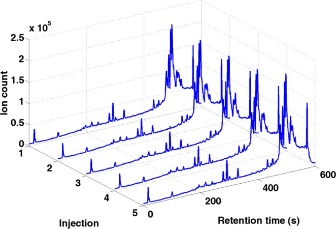
Total ion chromatogram of the five injections of the first aliquot of S1.
Then the peak list (list of peaks) from preprocessing was used to assess the variability among the repeated injections from an aliquot. For the first aliquot of biological subject S1 to S8, the logarithmic intensities of all the peaks from the first injection were compared against the logarithmic intensities of all the peaks from the other injections using scatter plots in Figure 2. The scatter plots of the peak intensities from two injections are largely on the diagonal line and exhibits a high correlation (Pearson Correlation =0.98; p < 0.001), indicating a high resemblance between the repeated injections. Since the five repeated injections span a time of 57.5 min, it is evident that the LC–MS system is stable over a short period of time.
Figure 2.

Evaluation of the variation due to the measurement noise. Scatter plots of logarithmic intensities of the five injections of the first aliquot of S1 to S8 represents (a) first injections vs second injections, (b) first injections vs third injections, (c) first injections vs fourth injections, and (d) first injections vs fifth injections.
The variance calculated from the ANOVA model and the coefficient of variation were compared along with m/z values and retention times to see if the measurement error of the LC–MS system is more significant over a particular region of chromatogram and mass spectrum, as sample preparation variation and interindividual variation should not be affected by chromatogram or mass measurement. Generally, the largest variation appears at the beginning (less than 25 seconds) of the chromatogram run (Figure 3). The reason for the large variation at the beginning of the chromatogram may be attributed to the high aqueous gradient of the reverse-phase chromatography that cannot retain the very polar compounds or hydrophilic metabolites in the beginning of the elution.50 If this area is considered to be important, it likely can be resolved by using HILIC (hydrophilic interaction liquid chromatography).51 The variation toward the end of the chromatogram is often observed partly due to baseline shift and can result in an overestimate of the intensities of the analytes.31 Thus, we have discarded the last two minutes of the chromatography during the preprocessing of the data. As shown in Figure 3, the retention time of peaks only go up to 480 s, where the variability of data is moderate. We also examined the variance along with peak intensities. The variation caused by the measurement noise shows a significant negative correlation (Spearman correlation = −0.66; p < 0.001, see Supplementary Figure 1, Supporting Information) with peak intensity. It is understandable as the noise effect is less severe on high-intensity peaks and it is relatively easy to detect and quantify high-intensity peaks. Coefficients of variation (CV) were determined. Overall, the mean CV for the measurement noise was 0.02, which ranged from 0.003 to 0.297. Similar to the above, the greatest CVs were in the areas at the beginning of the chromatogram. The correlation coefficient for the CV in relation to peak intensities is shown in Figure 4 (Spearman correlation = −0.785; p < 0.001). Those metabolites with CV more than 10% have been removed from the analysis for biomarker discovery.
Figure 3.
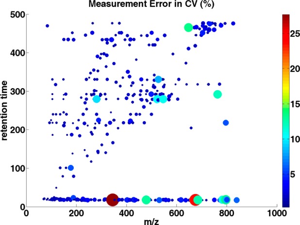
Distribution of the estimated measurement error in CV (%) over m/z values and retention times. Each dot represents a single peak. The dot size and color corresponds to the CV value: the larger the dot, and the brighter the color of the dot, the larger the CV value of the individual peak.
Figure 4.
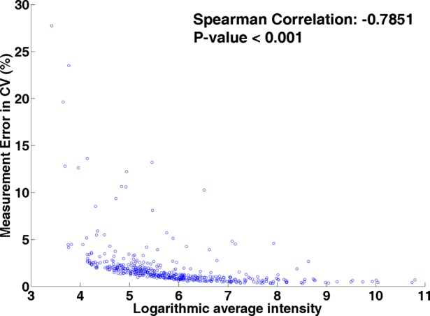
Scatter plot of the estimated measurement noise in coefficient of variation (%) versus the mean intensities of peaks over S1 to S8.
The scatter plot also was used to examine the variability due to sample preparation. The repeated injections from each aliquot were averaged to obtain the mean intensity of each peak for an aliquot. The logarithmic intensities of all peaks of the first aliquot of the eight biological subjects were compared with the logarithmic intensities of peaks of the second aliquot of the biological subjects. The two aliquots show a high degree of resemblance as the intensities are largely on the diagonal line (Supplementary Figure 2, Supporting Information) and exhibits a high correlation (Pearson Correlation = 0.99; p < 0.001). The results demonstrate that the sample preparation does not significantly affect the quality of the LC–MS data. Hierarchical clustering of the 8 subjects each with 8 injections (five plus three injections) from Experiment I is shown in Figure 5a. The clustering clearly distinguishes biological subjects but not injections from different aliquots. The result confirms that the variability due to sample preparation is generally equal to or smaller than the measurement error, so it is sometimes masked by the measurement error.
Figure 5.
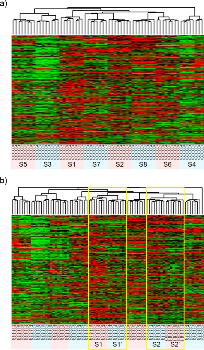
Hierarchical clustering of all metabolites (a) from subject 1 (S1) to subject 8 (S8) and (b) from S1 to S8 plus the analytical replicates S1′ and S2′. Heat map colors represent relative values, in which red represents values above the mean, black represents the mean, and green represents values below the mean of a row (metabolite) across all columns (samples).
2. Effects of Running Time and Carry-overs on Data Variability
In Experiment I, the first two biological subjects S1 and S2 were repeated at the end of the experiment as S1′ and S2′, with separate sample preparations and injections. Between S1 (S2) and S1′ (S2′), there were 56 other sample runs, and they were more than 10 h separated in time. The effects of run time and carry-overs on data variability can be evaluated by comparing S1 vs S1′ and S2 vs S2′. The logarithmic intensities of the four aliquots from S1 and S2 were compared with those of the four aliquots from S1′ and S2′. A high degree of resemblance is evident between S1, S2 and S1′, S2′ (Supplementary Figure 3, Supporting Information) and exhibits a high correlation (Pearson Correlation = 0.97; p < 0.001), which showcases that the LC–MS platform is stable after a moderate time period (more than 10 h).
We then analyzed a new hierarchical clustering adding experimental replicates (S1′ and S2′) that were run at the end of the experiment, and the result showed that the same sample’s analytical replicates were clustered together (S1 to S1′, and S2 to S2′, see Figure 5b). Thus, the increased running time and carry-overs of the sample analyzed between them does not significantly affect the data reproducibility. The estimated variances are shown as the box plot in Figure 6 and the variance and coefficient variation are summarized in Table 1. The results confirm that the variations between measurement error and sample preparation variation are comparable, while they are smaller than the interindividual variations, even if these replicates were analyzed 13 h apart.
Figure 6.
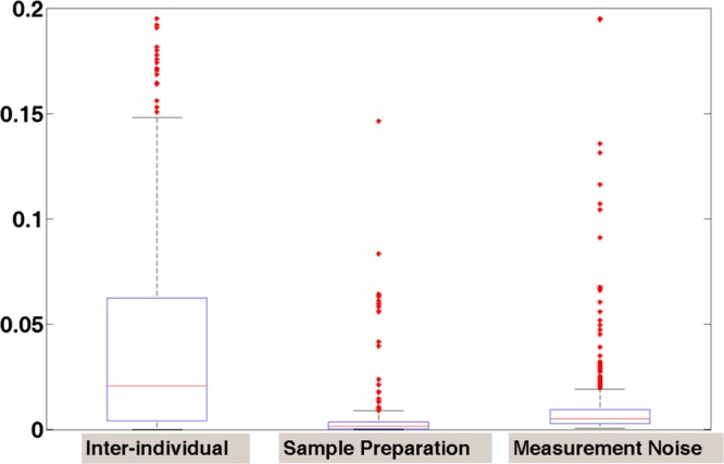
Box-plot of the estimated variances due to interindividual variation, sample preparation and measurement noise.
Table 1. Summary of the Measured Variance and Coefficient Variation in Human Plasma Samples.
| variance | CV | |
|---|---|---|
| mean (medium) | mean (medium) | |
| Interindividual variation | 0.068 (0.021) | 0.032 (0.025) |
| Sample preparation variation | 0.016 (0.002) | 0.011 (0.007) |
| Measurement noise | 0.021 (0.005) | 0.019 (0.013) |
From the model equation (1), we can deduce that the variance of the mean intensity of all the biological subjects is
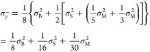 |
2 |
or more general
| 3 |
where I is number of biological subjects, j is the number of aliquots per subject and k is the number of injections per aliquot. This means that the variability of the mean of the observed peak intensity is dominated by the variation because of interindividual difference. Thus, the most effective way to reduce the variability in LC–MS data is to increase the number of biological subjects under investigation, given the total number of sample runs. Because of this understanding, in Experiment II, only one aliquot per subject and one injection per aliquot are used for the LC–MS-based metabolomics analysis of 613 biological subjects.
3. Reproducibility of LC–MS platform over multiple days
Experiment II provides the quality control data from a large metabolomics study of smokers (n = 160) with up to four separate blood draws before and after two cigarettes each (613 samples). For the quality control, 62 pooled healthy control samples were prepared by mixing equal volumes (400 μL) of plasma from seven nonsmokers and were inserted as every 10th sample of the run. Nonsmokers were used in order to assess background low level peaks. The pooled aliquot is assumed to be homogeneous and repeatedly injected across the entire LC–MS analysis with real biological samples analyzed between them. In Experiment II, 62 pooled quality control samples were injected during the analysis of 675 samples, including the 62 pooled samples. The analyses were conducted uninterrupted over 138 h. The peak list is acquired after peak detection and alignment using XCMS. It allows more in-depth analysis of LC–MS data. The preprocessing may help to reduce the variation in data due to instrument noise as only peak regions are considered in the analysis. This assesses reproducibility of the chromatography, quantitation of the spectroscopy, and run-to-run carryover and cross-contamination while running as a batch in a chromatographic system.
The reproducibility of the quality control replicates was analyzed through unsupervised principal component analysis (PCA) by MetaboAnalyst. PCA has been shown to be an effective approach to visualize high-dimensional data by projecting the data point into a low-dimension space. If a certain degree of platform stability has been attained, the QC samples should cluster tightly together in the PCA score plot. PCA of the experimental samples and QC samples has revealed a pattern as shown in Figure 7, which gives an indication about the reproducibility of the data. Although there are some variations among the QC samples, they occupy a relatively constrained space in the PCA score plot. When we compare our study (675 injections with 62 QCs, total run time 138 h) with the validation guideline for urine samples from Gika et al.36 and the same experiment presented by Want et al.38 (130 injections with 16 QCs, total run time 29 h), the performance of our QC samples showed little variation in tight clustering until samples run later in time. The deviation from the QC cluster might be due to the time-related drift in instrumental performance over a long time span in the large scale study,52,53 or the matrix effect due to the largely peptide/protein-based plasma samples compare to urine.54 Figure 8 is the hierarchical clustering analysis of samples and QCs shown as a heatmap using Pearson’s correlation for the similarity measure (distance), and clustering algorithms using Ward’s linkage (clustering to minimize the sum of squares of any two clusters). The result demonstrated that our platform is capable of discriminating the metabolome from clusters of QC samples and experimental samples, which again provides confidence in the quality of our pooled healthy controls throughout the run.
Figure 7.
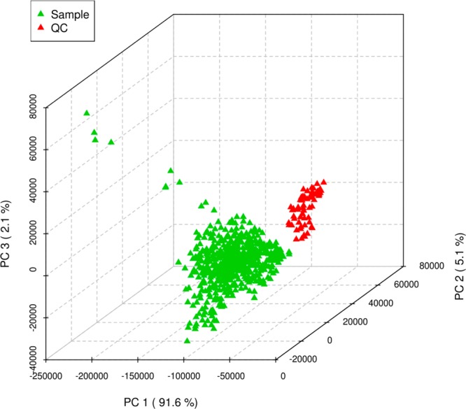
Scores plot between the selected principle components (PCs) showed difference between samples and QCs in their metabolomic profiles. The explained variances captured by each PC were shown in brackets.
Figure 8.

Clustering result shown as heatmap (distance measure using pearson, and clustering algorithm using ward) of the pooled QC samples and experimental samples.
4. Biomarkers Indicative of Smoking Behavior
There is wide interindividual variation for smoking behavior, which is affected by several factors such as race,55 gender,56 psychological factors57 and genetic background.58 Metabolomic profiling may identify differences in exposure and response, reflecting inherent biological differences. This could also lead to better prevention and early detection strategies. Metabolomics has the power to simultaneously detect carcinogen metabolites and endogenous metabolites affected by smoke exposure. Thus, both exposure and effect can be assessed. To examine the feasibility of a metabolomic study in assessing smoke exposure, Experiment III of 9 smokers and 10 nonsmokers was done using serum to evaluate differences of their global metabolomic profiles. Random Forests analysis was used to perform supervised classification and feature selection, and top 50 important features were selected with 100% accuracy by multidimensional scaling plot (Figure 9a) and can be visualized according to their rank importance (Figure 9b). To preliminarily identify the metabolites in Experiment III, the Madison-Qingdao Metabolomic Consortium Database and the Human Metabolome Database were searched; 169 putative features from the positive mode and 53 from the negative mode were identified. Then, 12 candidate metabolites were manually selected based on their putative identifications and availability of chemical standards for comparisons, as listed in Table 2. Validation for these candidate metabolites were then done by acquiring MS/MS spectra. As expected, the MS/MS spectra of nicotine, cotinine, 3-hydroxycotinine and cotinine N-oxide were verified and matched well with those from authentic compounds in our serum samples (Figure 10 and Supplementary Figure 4, Supporting Information). Nicotine is the major addictive component in cigarette smoke.59 In humans, it is primarily metabolized to cotinine by cytocrome P450 2A6 (CYP2A6) enzyme and further metabolized by the same enzyme to 3′-hydroxycotinine.60,61 Thus, the ratio of cotinine and 3′-hydroxycotinine reflect a stable CYP2A6 metabolic activity for nicotine metabolism.62 Pseudooxynicotine, 1,11-undecanedicarboxylic acid and 3-hydroxycoumarin were also verified by MS/MS identification. Pseudooxynicotine is an amino ketone product of nicotine by soil bacteria63,64 and was reported to be the direct precursor to the tobacco-specific lung carcinogen NNK in the bacterial systems.65 It was shown in vitro by Hecht et al. that the incubation of nicotine with human liver microsomes produced pseudooxynicotine through 2′-hydroxylation of nicotine63 but has not been identified in humans. Since microflora has been found to play a crucial role in human metabolome,66,67 tobacco-related metabolites metabolized by bacteria could have contributions to carcinogenesis that hadn’t been thought of before. Nicotine-related metabolites including nicotine, cotinine, 3-hydroxycotinine, cotinine N-oxide (a minor metabolite of nicotine) and pseudooxynicotine validated by MS/MS were all significantly higher in intensity among smokers compare to virtually zero among nonsmokers (Figure 11). In our results, 3-hydroxycoumarin and 11-undecanedicarboxylic acid were seen in both groups but higher in peak areas among nonsmokers compare to smokers (Figure 11). 3-Hydroxycoumarin is the metabolic product of the natural compound coumarin which can be found in plants and spices. Metabolism of coumarin in humans is mainly carried out by CYP2A6 to 7-hydroxycoumarin68 but also can be metabolized by CYP3A4 to 3-hydroxycoumarin.68 Nicotine is mainly metabolized by CYP2A6 enzyme, and thus could increase bioactivation of CYP2A6 and the 7-:3-hydroxycoumarin ratio among smokers. However, most of the reports on 3-hydroxycoumarin were done in rodent models and thus needs further clarification in human. 11-Undecanedicarboxylic acid is a dicarboxylic acid with a 13-carbon dibasic acid (tridecanedioic) occurring in plant and animal tissues. The relationship of 11-undecanedicarboxylic acid to cigarette smoke is still unknown, maybe through altering the carboxylic acid metabolism in the tobacco leaf or during the manufacture of cigarettes.
Figure 9.

Top 50 metabolites selected from Random Forests. (a) Forest accuracies were calculated and the sample classifications were presented by Multidimensional scaling (MDS) plot. In this plot, nonsmokers (red) and smokers (blue) were well separated in serum samples. (b) Visualization of the top metabolites across all samples identifies the rank importance of the ions.
Table 2. Candidate metabolites selected from 222 putative identifications differentiating smokers versus non-smokers.
| mode | metabolite ID | observed m/z | m/z | RT (min) | mass difference (in ppm) | smoker vs nonsmokers | HMDB ID |
|---|---|---|---|---|---|---|---|
| Positive | Cotinine | 177.10 | 176.09 | 0.35 | 4.89 | ↑ | HMDB01046 |
| 3-Hydroxycotinine | 193.10 | 192.09 | 0.36 | 4.92 | ↑ | HMDB01390 | |
| Cotinine N-oxide | 193.10 | 192.09 | 0.36 | 4.92 | ↑ | HMDB01411 | |
| Pseudooxynicotine | 179.12 | 178.11 | 0.71 | 3.43 | ↑ | HMDB01240 | |
| Nicotine | 163.12 | 162.12 | 0.51 | 6.32 | ↑ | HMDB14330 | |
| Cysteine-S-sulfate | 201.99 | 200.98 | 3.44 | 9.25 | ↓ | HMDB00731 | |
| 7a,12a-dihydroxy-3-oxo-4-cholenoic acid | 405.26 | 404.26 | 4.89 | 2.60 | ↓ | HMDB00447 | |
| Trans-3-hydroxycotinine glucuronide | 369.13 | 368.13 | 0.37 | 6.70 | ↑ | HMDB01204 | |
| Negative | Aminoparathion | 260.05 | 261.06 | 3.62 | 7.36 | ↑ | HMDB01504 |
| 1,11-Undecanedicarboxylic acid | 243.16 | 244.17 | 3.60 | 0.75 | ↓ | HMDB02327 | |
| 3-Hydroxycoumarin | 161.02 | 162.03 | 4.44 | 6.90 | ↓ | HMDB02149 | |
| Alpha-CEHC | 277.14 | 278.15 | 4.47 | 1.92 | ↓ | HMDB01518 |
Figure 10.

MS/MS spectrum from authentic compounds of cotinine (a1), hydroxycotinine (b1), pseudooxynicotine (c1), and 1,11-undecanedicarboxylic acid (d1). MS/MS spectrum obtained from serum samples of smoker (a2, b2, c2) or nonsmoker (d2) were also presented for comparison.
Figure 11.

Box plots of peak areas for seven candidate metabolites among smokers and nonsmokers. The points outside the quartiles are outliers.
Our results further show the feasibility and potential of the metabolomics profiling to identify new biomarkers of cigarette smoke exposure and lung cancer risk. Given that cigarette smoke is a complex mixture, it is possible that metabolic profiles will provide additional information for tobacco-related disease risk different from existing chemically specific biomarkers, such as those reported by Hecht et al.13 Also, broad detection methods such as used here can screen for unanticipated changes in smoke exposure as cigarette designs change. For example, the technology used to decrease some constituents might increase those of others (e.g., for the Eclipse cigarette,8 acrolein and CO increased69). Another reason for needing a broad biomarker such as a metabolomics profile of exposure and risk is to help tailor prevention and early detection strategies for former and current smokers. While this study will not directly assess biomarkers for lung cancer risk, the first step in developing these is the development of biomarkers of smoke exposures.47
Conclusions
Metabolomics provides information about the metabolic status of living systems and can provide phenotypic information about the cell’s environment and mechanistic pathways, as well as having clinical utility including as a risk biomarker.70−72 It is inexpensive and high-throughput, and has the potential to identify new biomarkers of cigarette smoke exposure and the consequent disease risk. Such biomarkers will assist in the evaluation of tobacco products and performance standards, and for identifying smokers at risk for lung cancer. Upon the basis of our study using UPLC–QTOF-MS, low variability is observed in measurement variation and sample preparation variation. When applying QC samples to the large scale study, QC clustering presents high stability of the platform but not the ones run later in time.
Various factors including the stability and maintenance of individual instrument, sample preparation techniques, and the choice of column could affect the performance of the chromatography result. Therefore, we recommend that for future metabolomics studies, especially large scale epidemiological studies, a separate experiment to assess the variability of the platform before applying precious human samples is needed so as not to exceed the results reported herein. After determining the required sample size, the number of aliquots and injections needed according to the variability of the specific platform, a pooled QC sample set to be run in between the experimental samples throughout the run is crucial in order to further assess the repeatability of the experiment. After preprocessing and analyzing the data, metabolites with CV no more than 10–15% should be considered for the biomarker discovery.
Metabolomics can potentially be used to better characterize smoking-related disease risks to enhance prevention and early detection methods, and by the FDA in the regulation of tobacco products. The recent authority to the FDA over tobacco products allows the FDA to mandate product performance standards governing smoke exposure to toxic constituents and also requires the FDA to evaluate manufacture’s health claims for modified-tobacco products of purported reduced exposure.5 The FDA decisions, however, will need to be supported by scientific studies and a better understanding of cigarette smoke toxicology. It also will require support through human studies and biomarkers that reflect the complex exposure to tobacco smoke. Today, though, there are only a few biomarkers of exposure and no validated biomarkers of cancer risk.73 As proof of principle, several new biomarkers were identified herein that have not thus far considered to be biomarkers of tobacco smoke exposure. Thus, metabolomics has the potential to develop a metabolic phenotype in healthy smokers of smoke exposure and disease risk.
Acknowledgments
We acknowledgment support from Transdisciplinary Tobacco Use Research Center grant P50 84718 from the National Cancer Institute and the National Institute on Drug Abuse, 1R01 CA114377–01A2, American Lung Association Lung Health Dissertation Grant (Ping-Ching Hsu) and NCI N01-PC-64402 - Laboratory Assessment of Tobacco Use Behavior and Exposure to Toxins.
Supporting Information Available
Supplemental figures.This material is available free of charge via the Internet at http://pubs.acs.org.
Author Contributions
‡ These authors contributed equally to this manuscript.
The authors declare the following competing financial interest(s): Dr. Shields serves as an expert witness in tobacco company litigation on behalf of plaintiffs. The other authors declare that they have no conflict of interest.
Funding Statement
National Institutes of Health, United States
Supplementary Material
References
- Department of Health U. S. Smoking and health. In The Surgeon General’s Report on Nutrition and Health; United States. Public Health Service. Office of the Surgeon General: Washington, D.C., 1988; pp 5–11. [Google Scholar]
- International Agency for Research on Cancer IARC Monographs on the Evaluation of Carcinogenic Risks to Humans; IARC: Lyon, France, 2004; pp 53–119. [PMC free article] [PubMed] [Google Scholar]
- International Agency for Research on Cancer. IARC Monographs on the Evaluation of the Carcinogenic Risk of Chemicals to Humans: Tobacco Smoking, Vol. 38; IARC: Lyon, 1986. [Google Scholar]
- Institute of Medicine; Committee to Assess the Science Base for Tobacco Harm Reduction; Board on Health Promotion and Disease Prevention Clearing the Smoke: Assessing the Science Base for Tobacco Harm Reduction; National Acadamy Press: Washington, D.C., 2001. [Google Scholar]
- Institute of Medicine; Committee to Assess the Science Base for Tobacco Harm Reduction; Board on Population Health and Public Health Practice. Scientific Standards for Studies on Modified Risk Tobacco Products. 2011. Ref Type: Report
- Centers for Disease Control and Prevention (US); Office on Smoking and Health (US). How Tobacco Smoke Causes Disease: The Biology and Behavioral Basis for Smoking-Attributable Disease: A Report of the Surgeon General; Atlanta, GA, 2010. [PubMed]
- Wan J.; Johnson M.; Schilz J.; Djordjevic M. V.; Rice J. R.; Shields P. G. Evaluation of in vitro assays for assessing the toxicity of cigarette smoke and smokeless tobacco. Cancer Epidemiol., Biomarkers Prev. 2009, 18, 3263–3304. [DOI] [PMC free article] [PubMed] [Google Scholar]
- Hatsukami D. K.; Benowitz N. L.; Rennard S. I.; Oncken C.; Hecht S. S. Biomarkers to assess the utility of potential reduced exposure tobacco products. Nicotine Tob. Res. 2006, 8, 600–622. [DOI] [PMC free article] [PubMed] [Google Scholar]
- Hoffmann D.; Hoffmann I.; El Bayoumy K. The less harmful cigarette: a controversial issue. a tribute to Ernst L. Wynder. Chem. Res. Toxicol. 2001, 14, 767–790. [DOI] [PubMed] [Google Scholar]
- International Agency for Research on Cancer. IARC Monographs on the Evaluation of Carcinogenic Risks to Humans; IARC: Lyon, France, 2004. [PMC free article] [PubMed] [Google Scholar]
- Smith C. J.; Perfetti T. A.; Garg R.; Hansch C. IARC carcinogens reported in cigarette mainstream smoke and their calculated log P values. Food Chem. Toxicol. 2003, 41, 807–817. [DOI] [PubMed] [Google Scholar]
- Hecht S. S. Tobacco smoke carcinogens and lung cancer. J. Natl. Cancer Inst. 1999, 91, 1194–1210. [DOI] [PubMed] [Google Scholar]
- Hecht S. S. Tobacco carcinogens, their biomarkers and tobacco-induced cancer. Nat. Rev. Cancer 2003, 3, 733–744. [DOI] [PubMed] [Google Scholar]
- Wright W. E.Epidemiology of occupations. In Environmental and Occupational Medicine; Rom W. N., Ed.; Little, Brown and Co.: Boston, 1983; pp 27–33. [Google Scholar]
- Fowles J.; Dybing E. Application of toxicological risk assessment principles to the chemical constituents of cigarette smoke. Tob. Control 2003, 12, 424–430. [DOI] [PMC free article] [PubMed] [Google Scholar]
- International Agency for Research on Cancer IARC Monographs on the Evaluation of Carcinogenic Risks to Humans; International Agency on the Research of Cancer: Lyon, France, 1982; pp 93–148. [Google Scholar]
- Chen C.; Gonzalez F. J.; Idle J. R. LC-MS-based metabolomics in drug metabolism. Drug Metab. Rev. 2007, 39, 581–597. [DOI] [PMC free article] [PubMed] [Google Scholar]
- Idle J. R.; Gonzalez F. J. Metabolomics. Cell Metab. 2007, 6, 348–351. [DOI] [PMC free article] [PubMed] [Google Scholar]
- Kaddurah-Daouk R.; Kristal B. S.; Weinshilboum R. M. Metabolomics: a global biochemical approach to drug response and disease. Annu. Rev. Pharmacol. Toxicol. 2008, 48, 653–683. [DOI] [PubMed] [Google Scholar]
- Bain J. R.; Stevens R. D.; Wenner B. R.; Ilkayeva O.; Muoio D. M.; Newgard C. B. Metabolomics applied to diabetes research: moving from information to knowledge. Diabetes 2009, 58, 2429–2443. [DOI] [PMC free article] [PubMed] [Google Scholar]
- Griffin J. L. The Cinderella story of metabolic profiling: does metabolomics get to go to the functional genomics ball?. Philos. Trans. R. Soc. Lond. B: Biol. Sci. 2006, 361, 147–161. [DOI] [PMC free article] [PubMed] [Google Scholar]
- Lewis G. D.; Asnani A.; Gerszten R. E. Application of metabolomics to cardiovascular biomarker and pathway discovery. J. Am. Coll. Cardiol. 2008, 52, 117–123. [DOI] [PMC free article] [PubMed] [Google Scholar]
- Fernie A. R.; Trethewey R. N.; Krotzky A. J.; Willmitzer L. Metabolite profiling: from diagnostics to systems biology. Nat. Rev. Mol. Cell Biol. 2004, 5, 763–769. [DOI] [PubMed] [Google Scholar]
- Nicholson J. K.; Wilson I. D. Opinion: understanding ’global’ systems biology: metabonomics and the continuum of metabolism. Nat. Rev. Drug Discov. 2003, 2, 668–676. [DOI] [PubMed] [Google Scholar]
- Griffin J. L. The Cinderella story of metabolic profiling: does metabolomics get to go to the functional genomics ball?. Philos. Trans. R. Soc. Lond. B: Biol. Sci. 2006, 361, 147–161. [DOI] [PMC free article] [PubMed] [Google Scholar]
- Weckwerth W.Metabolomics: methods and protocols; Springer-Verlag: New York, 2006. [Google Scholar]
- Kanani H.; Chrysanthopoulos P. K.; Klapa M. I. Standardizing GC-MS metabolomics. J. Chromatogr. B Analyt. Technol. Biomed. Life Sci. 2008, 871, 191–201. [DOI] [PubMed] [Google Scholar]
- Kaddurah-Daouk R.; Boyle S.; Matson W.; Sharma S.; Matson S.; Zhu H.; Bogdanov M.; Churchill E.; Krishnan R.; Rush A.; Pickering E.; Delnomdedieu M.. Pretreatment metabotype as a predictor of response to sertraline or placebo in depressed outpatients: a proof of concept. Transl. Psychiatry 2011, 1. [DOI] [PMC free article] [PubMed] [Google Scholar]
- O’Grady J.; Schwender J.; Shachar-Hill Y.; Morgan J. A. Metabolic cartography: experimental quantification of metabolic fluxes from isotopic labelling studies. J. Exp. Bot. 2012, 63, 2293–2308. [DOI] [PubMed] [Google Scholar]
- Reo N. V. NMR-based metabolomics. Drug Chem. Toxicol. 2002, 25, 375–382. [DOI] [PubMed] [Google Scholar]
- Zhou B.; Xiao J. F.; Tuli L.; Ressom H. W. LC-MS-based metabolomics. Mol. Biosyst. 2012, 8, 470–481. [DOI] [PMC free article] [PubMed] [Google Scholar]
- Psychogios N.; Hau D. D.; Peng J.; Guo A. C.; Mandal R.; Bouatra S.; Sinelnikov I.; Krishnamurthy R.; Eisner R.; Gautam B.; Young N.; Xia J.; Knox C.; Dong E.; Huang P.; Hollander Z.; Pedersen T. L.; Smith S. R.; Bamforth F.; Greiner R.; McManus B.; Newman J. W.; Goodfriend T.; Wishart D. S. The human serum metabolome. PLoS One 2011, 6, e16957. [DOI] [PMC free article] [PubMed] [Google Scholar]
- Bathe O. F.; Shaykhutdinov R.; Kopciuk K.; Weljie A. M.; McKay A.; Sutherland F. R.; Dixon E.; Dunse N.; Sotiropoulos D.; Vogel H. J. Feasibility of identifying pancreatic cancer based on serum metabolomics. Cancer Epidemiol. Biomarkers Prev. 2011, 20, 140–147. [DOI] [PubMed] [Google Scholar]
- Ciborowski M.; Javier R. F.; Martinez-Alcazar M. P.; Angulo S.; Radziwon P.; Olszanski R.; Kloczko J.; Barbas C. Metabolomic approach with LC–MS reveals significant effect of pressure on diver’s plasma. J. Proteome Res. 2010, 9, 4131–4137. [DOI] [PubMed] [Google Scholar]
- Sato Y.; Suzuki I.; Nakamura T.; Bernier F.; Aoshima K.; Oda Y. Identification of a new plasma biomarker of Alzheimer’s disease using metabolomics technology. J. Lipid Res. 2012, 53, 567–576. [DOI] [PMC free article] [PubMed] [Google Scholar]
- Gika H. G.; Macpherson E.; Theodoridis G. A.; Wilson I. D. Evaluation of the repeatability of ultra-performance liquid chromatography-TOF-MS for global metabolic profiling of human urine samples. J. Chromatogr.. B: Anal. Technol. Biomed. Life Sci. 2008, 871, 299–305. [DOI] [PubMed] [Google Scholar]
- Guy P. A.; Tavazzi I.; Bruce S. J.; Ramadan Z.; Kochhar S. Global metabolic profiling analysis on human urine by UPLC-TOFMS: issues and method validation in nutritional metabolomics. J. Chromatogr., B: Anal. Technol. Biomed. Life Sci. 2008, 871, 253–260. [DOI] [PubMed] [Google Scholar]
- Want E. J.; Wilson I. D.; Gika H.; Theodoridis G.; Plumb R. S.; Shockcor J.; Holmes E.; Nicholson J. K. Global metabolic profiling procedures for urine using UPLC-MS. Nat. Protoc. 2010, 5, 1005–1018. [DOI] [PubMed] [Google Scholar]
- Gika H. G.; Theodoridis G. A.; Wingate J. E.; Wilson I. D. Within-day reproducibility of an HPLC–MS-based method for metabonomic analysis: application to human urine. J. Proteome Res. 2007, 6, 3291–3303. [DOI] [PubMed] [Google Scholar]
- Crews B.; Wikoff W. R.; Patti G. J.; Woo H. K.; Kalisiak E.; Heideker J.; Siuzdak G. Variability analysis of human plasma and cerebral spinal fluid reveals statistical significance of changes in mass spectrometry-based metabolomics data. Anal. Chem. 2009, 81, 8538–8544. [DOI] [PMC free article] [PubMed] [Google Scholar]
- Smith C. A.; Want E. J.; O’Maille G.; Abagyan R.; Siuzdak G. XCMS: processing mass spectrometry data for metabolite profiling using nonlinear peak alignment, matching, and identification. Anal. Chem. 2006, 78, 779–787. [DOI] [PubMed] [Google Scholar]
- Xia J.; Psychogios N.; Young N.; Wishart D. S. MetaboAnalyst: a web server for metabolomic data analysis and interpretation. Nucleic Acids Res. 2009, 37, W652–W660. [DOI] [PMC free article] [PubMed] [Google Scholar]
- Cui Q.; Lewis I. A.; Hegeman A. D.; Anderson M. E.; Li J.; Schulte C. F.; Westler W. M.; Eghbalnia H. R.; Sussman M. R.; Markley J. L. Metabolite identification via the Madison Metabolomics Consortium Database. Nat. Biotechnol. 2008, 26, 162–164. [DOI] [PubMed] [Google Scholar]
- Wishart D. S. Human Metabolome Database: completing the ’human parts list’. Pharmacogenomics 2007, 8, 683–686. [DOI] [PubMed] [Google Scholar]
- Wedge D. C.; Allwood J. W.; Dunn W.; Vaughan A. A.; Simpson K.; Brown M.; Priest L.; Blackhall F. H.; Whetton A. D.; Dive C.; Goodacre R. Is serum or plasma more appropriate for intersubject comparisons in metabolomic studies? An assessment in patients with small-cell lung cancer. Anal. Chem. 2011, 83, 6689–6697. [DOI] [PubMed] [Google Scholar]
- Yu Z.; Kastenmuller G.; He Y.; Belcredi P.; Moller G.; Prehn C.; Mendes J.; Wahl S.; Roemisch-Margl W.; Ceglarek U.; Polonikov A.; Dahmen N.; Prokisch H.; Xie L.; Li Y.; Wichmann H. E.; Peters A.; Kronenberg F.; Suhre K.; Adamski J.; Illig T.; Wang-Sattler R. Differences between human plasma and serum metabolite profiles. PLoS One 2011, 6, e21230. [DOI] [PMC free article] [PubMed] [Google Scholar]
- Hatsukami D. K.; Slade J.; Benowitz N. L.; Giovino G. A.; Gritz E. R.; Leischow S.; Warner K. E. Reducing tobacco harm: research challenges and issues. Nicotine Tob. Res. 2002, 4, S89–S101. [DOI] [PubMed] [Google Scholar]
- Oberg A. L.; Vitek O. Statistical design of quantitative mass spectrometry-based proteomic experiments. J. Proteome Res. 2009, 8, 2144–2156. [DOI] [PubMed] [Google Scholar]
- Smilde A. K.; van der Werf M. J.; Schaller J. P.; Kistemaker C. Characterizing the precision of mass-spectrometry-based metabolic profiling platforms. Analyst 2009, 134, 2281–2285. [DOI] [PubMed] [Google Scholar]
- Dettmer K.; Aronov P. A.; Hammock B. D. Mass spectrometry-based metabolomics. Mass Spectrom. Rev. 2007, 26, 51–78. [DOI] [PMC free article] [PubMed] [Google Scholar]
- Jameson D.; Verma M.; Westerhoff H. V.. Methods in Systems Biology; Academic Press: New York, 2012; Vol. 500, p 21. [Google Scholar]
- Lange E.; Tautenhahn R.; Neumann S.; Gropl C. Critical assessment of alignment procedures for LC-MS proteomics and metabolomics measurements. BMC Bioinform. 2008, 9, 375. [DOI] [PMC free article] [PubMed] [Google Scholar]
- Zelena E.; Dunn W. B.; Broadhurst D.; Francis-McIntyre S.; Carroll K. M.; Begley P.; O’Hagan S.; Knowles J. D.; Halsall A.; Wilson I. D.; Kell D. B. Development of a robust and repeatable UPLC-MS method for the long-term metabolomic study of human serum. Anal. Chem. 2009, 81, 1357–1364. [DOI] [PubMed] [Google Scholar]
- Denery J. R.; Nunes A. A.; Dickerson T. J. Characterization of differences between blood sample matrices in untargeted metabolomics. Anal. Chem. 2011, 83, 1040–1047. [DOI] [PubMed] [Google Scholar]
- Ahijevych K.; Gillespie J.; Demirci M.; Jagadeesh J. Menthol and nonmenthol cigarettes and smoke exposure in black and white women. Pharmacol., Biochem. Behav. 1996, 53, 355–360. [DOI] [PubMed] [Google Scholar]
- Assaf A. R.; Parker D.; Lapane K. L.; McKenney J. L.; Carleton R. A. Are there gender differences in self-reported smoking practices? Correlation with thiocyanate and cotinine levels in smokers and nonsmokers from the Pawtucket Heart Health Program. J. Womens Health 2002, 11, 899–906. [DOI] [PubMed] [Google Scholar]
- Lombardo T.; Carreno L. Relationship of type A behavior pattern in smokers to carbon monoxide exposure and smoking topography. Health Psychol. 1987, 6, 445–452. [DOI] [PubMed] [Google Scholar]
- Lerman C.; Berrettini W. Elucidating the role of genetic factors in smoking behavior and nicotine dependence. Am. J. Med. Genet. B: Neuropsychiatr. Genet. 2003, 118B, 48–54. [DOI] [PubMed] [Google Scholar]
- Benowitz N. L. Nicotine addiction. Prim. Care 1999, 26, 611–631. [DOI] [PubMed] [Google Scholar]
- Messina E. S.; Tyndale R. F.; Sellers E. M. A major role for CYP2A6 in nicotine C-oxidation by human liver microsomes. J. Pharmacol. Exp. Ther. 1997, 282, 1608–1614. [PubMed] [Google Scholar]
- Nakajima M.; Yamamoto T.; Nunoya K.; Yokoi T.; Nagashima K.; Inoue K.; Funae Y.; Shimada N.; Kamataki T.; Kuroiwa Y. Characterization of CYP2A6 involved in 3′-hydroxylation of cotinine in human liver microsomes. J. Pharmacol. Exp. Ther. 1996, 277, 1010–1015. [PubMed] [Google Scholar]
- Dempsey D.; Tutka P.; Jacob P. III; Allen F.; Schoedel K.; Tyndale R. F.; Benowitz N. L. Nicotine metabolite ratio as an index of cytochrome P450 2A6 metabolic activity. Clin. Pharmacol. Ther. 2004, 76, 64–72. [DOI] [PubMed] [Google Scholar]
- Hecht S. S.; Hochalter J. B.; Villalta P. W.; Murphy S. E. 2′-Hydroxylation of nicotine by cytochrome P450 2A6 and human liver microsomes: formation of a lung carcinogen precursor. Proc. Natl. Acad. Sci. U.S.A. 2000, 97, 12493–12497. [DOI] [PMC free article] [PubMed] [Google Scholar]
- Wada E. Y. K. Degradation of Nicotine by Soil Bacteria. J. Am. Chem. Soc. 1954, 76, 155–157. [Google Scholar]
- Caldwell W. S.; Greene J. M.; Dobson G. P.; deBethizy J. D. Intragastric nitrosation of nicotine is not a significant contributor to nitrosamine exposure. Ann. N.Y. Acad. Sci. 1993, 686, 213–227. [DOI] [PubMed] [Google Scholar]
- Holmes E.; Li J. V.; Athanasiou T.; Ashrafian H.; Nicholson J. K. Understanding the role of gut microbiome-host metabolic signal disruption in health and disease. Trends Microbiol. 2011, 19, 349–359. [DOI] [PubMed] [Google Scholar]
- Wikoff W. R.; Anfora A. T.; Liu J.; Schultz P. G.; Lesley S. A.; Peters E. C.; Siuzdak G. Metabolomics analysis reveals large effects of gut microflora on mammalian blood metabolites. Proc. Natl. Acad. Sci. U.S.A. 2009, 106, 3698–3703. [DOI] [PMC free article] [PubMed] [Google Scholar]
- Lewis D. F.; Ito Y.; Lake B. G. Metabolism of coumarin by human P450s: a molecular modelling study. Toxicol. In Vitro 2006, 20, 256–264. [DOI] [PubMed] [Google Scholar]
- Strasser A. A.; Lerman C.; Sanborn P. M.; Pickworth W. B.; Feldman E. A. New lower nicotine cigarettes can produce compensatory smoking and increased carbon monoxide exposure. Drug Alcohol Depend. 2007, 86, 294–300. [DOI] [PubMed] [Google Scholar]
- Ceglarek U.; Leichtle A.; Brugel M.; Kortz L.; Brauer R.; Bresler K.; Thiery J.; Fiedler G. M. Challenges and developments in tandem mass spectrometry based clinical metabolomics. Mol. Cell. Endocrinol. 2009, 301, 266–271. [DOI] [PubMed] [Google Scholar]
- Serkova N. J.; Glunde K. Metabolomics of cancer. Methods Mol. Biol. 2009, 520, 273–295. [DOI] [PubMed] [Google Scholar]
- Spratlin J. L.; Serkova N. J.; Eckhardt S. G. Clinical applications of metabolomics in oncology: a review. Clin. Cancer Res. 2009, 15, 431–440. [DOI] [PMC free article] [PubMed] [Google Scholar]
- Hatsukami D. K.; Benowitz N. L.; Rennard S. I.; Oncken C.; Hecht S. S. Biomarkers to assess the utility of potential reduced exposure tobacco products. Nicotine Tob. Res. 2006, 8, 169–191. [DOI] [PubMed] [Google Scholar]
Associated Data
This section collects any data citations, data availability statements, or supplementary materials included in this article.