Reduced atomic pair-interaction design (RAPID) model for simulations of proteins

Abstract

Increasingly, theoretical studies of proteins focus on large systems. This trend demands the development of computational models that are fast, to overcome the growing complexity, and accurate, to capture the physically relevant features. To address this demand, we introduce a protein model that uses all-atom architecture to ensure the highest level of chemical detail while employing effective pair potentials to represent the effect of solvent to achieve the maximum speed. The effective potentials are derived for amino acid residues based on the condition that the solvent-free model matches the relevant pair-distribution functions observed in explicit solvent simulations. As a test, the model is applied to alanine polypeptides. For the chain with 10 amino acid residues, the model is found to reproduce properly the native state and its population. Small discrepancies are observed for other folding properties and can be attributed to the approximations inherent in the model. The transferability of the generated effective potentials is investigated in simulations of a longer peptide with 25 residues. A minimal set of potentials is identified that leads to qualitatively correct results in comparison with the explicit solvent simulations. Further tests, conducted for multiple peptide chains, show that the transferable model correctly reproduces the experimentally observed tendency of polyalanines to aggregate into β-sheets more strongly with the growing length of the peptide chain. Taken together, the reported results suggest that the proposed model could be used to succesfully simulate folding and aggregation of small peptides in atomic detail. Further tests are needed to assess the strengths and limitations of the model more thoroughly.

INTRODUCTION

Continuing progress in the development of computer technology and availability of fast and hardware-customizable simulation packages¹ make it possible for present-day computational studies of proteins to focus increasingly on large systems.² Of particular interest in this context are large multi-domain proteins, such as chaperons or motor proteins,³ protein complexes,⁴ and proteins that undergo aggregation.⁵ The success of computational approaches to large systems depends on the usual trade-off between the complexity of the employed protein models and their speeds. Atomically accurate models are the slowest. When combined with the explicit solvent representation, they typically allow for simulations on nanosecond time scale.^{6, 7, 8} To extend the accessible simulation time, models with reduced representations are needed. The pertinent question in designing such models, which vary widely in complexity,^{9, 10, 11, 12, 13} is that “What level of simplification is justified for the given problem?”. Growing body of evidence shows that both folding and aggregation pathways are very sensitive to the chemical detail of the protein's primary sequence. A conservative F-to-A mutation at a critical location in the myosin motor protein, for example, is seen to completely abolish the motor function by decoupling the active site from the force-generating region.¹⁴ Aggregation studies of amyloid β peptide¹⁵ report a comparable by magnitude effect, where A-for-I or V-for-I mutations cause substantial redistribution in the equilibrium population of various oligomeric species. The small chemical differences between the concerned residues in both cases suggest that atomistic protein representation is required to properly reproduce the observed behavior, if not quantitatively then at least qualitatively.

The simplification at the atomic level concerns only the solvent in which proteins are modeled. Solvent, most often water, can be treated in a variety of ways, but most frequently it is completely removed and replaced by effective potentials ΔG acting on the protein molecule and known as the solvation free energy.¹⁶ Although a large number of solvation models have been introduced for biomolecular simulations,¹⁷ the scheme that separates ΔG into electrostatic, ΔG_el, and non-polar, ΔG_np, components based on certain physical principles is among the most successful. Within this scheme, very accurate approximations are available for ΔG_el derived with the help of continuum electrostatics model,^{18, 19} whereas the theory of non-polar solvation ΔG_np is relatively less developed.^{20, 21, 22, 23} The most widely accepted^{22, 24} non-polar solvation model is based on solvent-accessible surface area (SASA). Importantly, both these models, electrostatics and non-polar, contain multi-particle interactions that lead to very slow computations. Implicit solvent simulations of large proteins using these models may run even slower than the corresponding simulations in explicit solvent.²⁵

An alternative to the physics-based solvation free energy is statistical potentials.²⁶ Instead of providing a universal solvation model that fits all proteins, these potentials are derived specifically for the given system of interest and depend on its thermodynamic state. Most importantly, the statistical potentials can be chosen short-ranged and pair-wise additive, a property that adds no cost to the computations which already contain dispersive interactions. Simulations employing such potentials thus run at the maximum speed compatible with the chosen protein architecture. While not without limitations, the pair-wise approximation has been used successfully in a variety of condensed matter, colloidal, and polymer systems.^{27, 28} In particular, the statistical pair potentials were recently derived for electrolyte solutions,²⁹ nucleic acids,³⁰ small peptides,^{31, 32} lipids,³³ and a host of synthetic polymers.^{34, 35, 36, 37, 38}

In the studies of large proteins and their assemblies the statistical approach is relevant in at least two contexts. First, it permits the studies of large proteins composed of a repeat fragment, if the fragment is sufficiently small to allow for the derivation of effective potentials from explicit solvent simulations. Examples of such systems are homo polypeptides, including polyalanine (poly-A), polyglutamine (poly-Q), and polyasparagine (poly-N), all of which are biologically relevant.^{39, 40} Second, statistical potentials can be derived for short peptides in order to study their aggregation. Although a variety of recently introduced models can simulate spontaneous self-assembly of peptides into β-rich aggregates,^{41, 42, 43, 44, 45} only a small number of them can do so in atomic detail.^{46, 47, 48, 49, 50, 51, 52} Of these latter studies, only one model^{50, 51, 52} has the speed and accuracy necessary for the simulation of self-assembling multi-layered β-sheets reminiscent of protofibrils observed experimentally.^{53, 54}

In this paper we introduce a model for simulations of long polypeptides and their assemblies based on the reduced atomic pair-interaction design (RAPID) strategy. As its name implies, the proposed model uses all-atom protein architecture coupled with a standard protein force-field.⁵⁵ The electrostatic component ΔG_el of the solvation free energy is included through a distance-dependent dielectric constant. The remaining part, which includes non-polar energy and possible errors in ΔG_el, is represented by pair potentials applied to hydrophobic moieties of the peptide. The potentials are derived systematically by matching pair distribution functions among hydrophobic sites obtained in implicit and explicit solvent simulations. The model is tested for polyalanine decapeptide solvated in water. The peptide is shown in explicit solvent simulations to remain mostly in random-coil conformations with small population of α-helical states. The same characteristics of the conformational ensemble are observed in the implicit solvent model. Small discrepancies between explicit and implicit treatments are seen in the distribution of the helical structure along the sequence. The transferability of the derived implicit solvation model is tested in simulations of larger peptides. A model with a minimal number of potential energy terms is identified that satisfactorily represents folding of polyalanine chain with 25 residues. As a final test, multi-peptide systems are simulated. In agreement with experiment,^{40, 56} 8 chains of varying lengths are observed to form double-layer β-sheet as the most populated state, proving that the proposed model is suitable for theoretical studies of protein aggregation.

METHODS AND MODELS

Structure-based methods for deriving effective potentials

The protein solvation energy will be computed in this work using methods of structure-based statistical potentials developed in the theory of soft matter systems.⁵⁷ The main goal is to find an effective pair potential u_eff(r) that reproduces known pair distribution function g(r). Historically, the effective potentials were first derived for simple liquids with known experimental structural functions.^{58, 59, 60, 61} In these systems, the pair-wise approximation, $U_e={\sum }_{i,j}{u}_{eff}\left(r_{ij}\right)$, where the summation runs over all pairs of particles, is designed to mimic the actual potential energy function that may contain multi-body contributions, $U_T({\vec{r}}_1...,{\vec{r}}_N)={\sum }_{i,j}{u}^2\left(r_{ij}\right)+{\sum }_{i,j,k}{u}^3(r_{ij},r_{ik},r_{jk})+...,$ where ${\vec{r}}_1,...,{\vec{r}}_N$ are the coordinates of N particles and u² and u³ are two- and three-body interactions. More recently, the same methodology has been applied to the problem of constructing simplified models of soft-matter systems that are too complex to be studied in atomic detail,^{30, 31, 32, 33} or the so-called coarse-graining. In this approach, the potential energy U_T is replaced with the free energy, which, in addition to the direct physical interactions among selected degrees of freedom, also includes the effect of the degrees of freedom that are integrated out in the course of the coarse-graining. The splitting of U_T into multi-body contributions is not unique but can be introduced in a consistent way. To facilitate the discussion of the model further down the text, we will assume that the interacting particles resulting from the coarse-graining have full translational freedom. As free energy, U_T depends on the thermodynamic variables of the studied system, including the density of the coarse-grained particles. The splitting into multi-body terms can be accomplished by analogy to the simple liquids in the zero-density limit. Let u² be associated with the free energy of only two coarse-grained particles, u³ be taken to represent free energy of three particles not captured by the two-particle term while higher-order terms be designed similarly to the three-body term. In this way, a complete set of density-independent multi-body potentials (up to the order N, u^N) can be obtained. The resulting potential $U_D={\sum }_{i,j}{u}^2\left(r_{ij}\right)+{\sum }_{i,j,k}{u}^3(r_{ij},r_{ik},r_{jk})+...+u^N({\vec{r}}_1,...,{\vec{r}}_N)$ has to be corrected with the term ${\delta }_N({\vec{r}}_1,...,{\vec{r}}_N)=U_T-U_D$ in order to match the target free energy U_T = U_D + δ_N. The correction term encapsulates the dependence of the free energy on density and vanishes in the low-density limit. The proposed scheme allows for both simple liquids and coarse-grained systems to be treated on equal theoretical footing.

The uniqueness theorem⁶² establishes a one-to-one correspondence between a pair potential and the pair distribution function it generates. Thus, the effective potentials u_eff(r) can be derived from known g(r) (available either from experiments or high-resolution simulations) by solving the inverse problem of statistical mechanics: “Starting from the known structure g(r), find the corresponding potential u(r).” A number of numerical implementations have been devised to address this problem, including the older approaches based on the integral-equation theory of liquid state⁶⁰ and the more recent ones^{61, 63} that rely on numerical Monte Carlo inversion. We will use the Monte Carlo based methods here because of their superior accuracy demonstrated in applications to a wide range of systems, including electrolyte solutions,²⁹ nucleic acids,³⁰ peptides,^{31, 32} lipids,³³ and a host of synthetic polymers.^{34, 35, 36, 37} In a multi-component system, the potential u^αβ(r_ij) acting between particle i of species α and particle j of species β will be determined iteratively using the following recurrent relationship:^{58, 59, 61}

$$u_{l+1}^{\alpha \beta }\left(r_{ij}\right)=u_l^{\alpha \beta }\left(r_{ij}\right)-{\lambda }_{l}kT\log \left(\frac{g_R^{\alpha \beta }\left(r_{ij}\right)}{g_l^{\alpha \beta }\left(r_{ij}\right)}\right),$$ (1)

where index l numbers successive iterations, $g_R^{\alpha \beta }\left(r\right)$ is the reference pair distribution function obtained in a higher-level atomic simulation, k is the Boltzmann constant, T is the simulation temperature, and $g_l^{\alpha \beta }\left(r\right)$ is the distribution function obtained for the current iteration. We note that this relationship ignores the effect of the pair distribution function of one type on the potential derived for the pair of atoms of another type. It is known that the lack of such cross-correlation may cause slow convergence in multi-component systems.⁶⁴ To overcome this problem we (a) designed the initial guess of the potential to be of high quality (judged by the distribution functions), and (b) introduced coefficient λ_l that was varied manually between 0 and 1 in the course of the iterations in order to control the convergence rate. The exact numerical value of λ_l does not affect the converged potential as in that case $g_R^{\alpha \beta }\left(r\right)=g^{\alpha \beta }\left(r\right)$ and the logarithm in Eq. 1 vanishes. We also performed several independent tests using different sets of initial potentials to check the convergence of the algorithm, as discussed in Sec. 3.

As an approximation to the free energy, the effective potentials u_eff(r) depend on the thermodynamic parameters of the studied system such as density and temperature. The density enters through multi-body interactions (including the explicit dependence in the correction term δ_N), which are approximated at the pair-wise level. In the condensed phases, where collisions among more than 2 particles are common, the multi-particle potentials play an important role. As the density decreases, however, their influence diminishes since multi-particle configurations become much less frequent than binary collisions. In the limit of low density (the gaseous phase), the contribution of the multi-body potentials is negligible. The effective potentials then report on the properly defined two-body potential u²(r). This convergence can be used to extract density independent u²(r) from density-dependent studies.

For the sake of completeness, we note an alternative approach to coarse-graining that is based on a force-matching algorithm of Ercolessi and Adams.⁶⁵ Introduced originally to derive classical potentials from quantum mechanical simulations, this method was further developed by Voth and Izvekov⁶⁶ and applied to a large class of biomolecular systems, including peptides,⁶⁷ sugars,⁶⁸ and phosphilipids.⁶⁹

Effective potentials for homopolymers

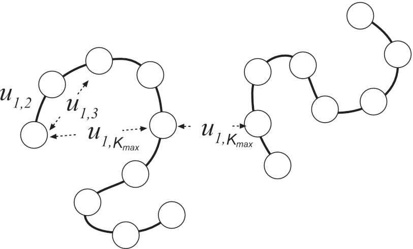
The fact that the effective potentials depend on thermodynamic parameters has important consequences for the application of coarse-graining to polymers. Let us consider for simplicity generic homopolymers created by polymerization of some chemical compound, for instance, amino acids in polypeptides. Although all the units in such a polymer are chemically equivalent, they have to be treated as distinct species during coarse-graining because of the chain connectivity. Consider an illustration in Figure 1 showing a polymer with particles numbered from 1 to N. Focusing on particle 1, it is easy to see that the local density created by particle with number 2 will be different from the density of particle number 3, particle number 4, and so on. The same argument applies to any particle I, generating a total of N(N − 1)/2 potentials specific to each pair of residues, u_{i, j}, i = 1, N − 1, j = i + 1, N.

Figure 1.

Effective intra-molecular potentials in homopolymers. The dependence on how far the residues are separated along the sequence drops for sufficiently long sequences. One potential then describes both intra- and inter-peptide interactions.

In general, all of these potentials have to be treated as distinct. However, the difference between some of them will be small or unimportant. Consider the nearest neighbors terms u_{i, i+1}. Clearly these potentials will depend on the exact location of the affected pair in the sequence. Because of the finite length of the polymer, u_1,2 at the beginning of the sequence, for instance, will be different from u_{N/2, N/2+1} in the middle of the sequence. As a boundary effect, however, the difference will not strongly impact the overall conformational statistics of the polymer in the limit of large N, so it can be neglected. We will assume that the same arguments apply to all other neighbors and treat the potential u_{i, j} as depending only on the number of residues separating i and j,u_i−j. This assumption reduces the number of independent potentials from N(N − 1)/2 to N − 1.

Further, it is easy to see that not all of these potentials are different. Let us focus on the potentials applied to particle 1 once again, as shown in Figure 1. The second neighbors along the chain will create a lower effective density than the first neighbors. This trend will continue for longer neighbors, which will exhibit increasingly low density with the separation from residue 1. Starting at certain position, the neighbors will become de-correlated, indicating a distance longer than the persistence length.⁷⁰ Such neighbors will effectively appear the same to the first particle, implying that they should interact with the same potential. For sufficiently long distances (along the sequence), starting at numberK_max, there should be a convergence in the effective potentials^{35, 36} such that $u_{i-j}=u_{1,K_{\max }},i-j\ge K_{\max }-1$. An important difference here with the liquids is that the limiting effective potential in polymers is not equal to the density-independent pair potential acting between constituent units of the polymer, $u_{1-K_{\max }}\left(r\right)\ne u^2\left(r\right)$. Although the density of remote neighbors goes to zero, the relative contribution of multi-particle configurations does not, due to the chain connectivity. Every time a neighbor j > K_max interacts with the particle 1, it also interacts with the particles strongly correlated to it, such as 2, 3, and so on. Unlike liquids, therefore, the impact of multi-particle potentials in polymers never vanishes. Consequently, the effective potentials derived for polymers will always contain multi-particle contributions.

Both the convergence length K_max and the total number of unique potentials depend on the basic properties of the studied polymer such as the chemistry of amino acid residues, the length, and the thermodynamic state. If a polymer is used for the extraction of effective potentials, its size N_t must be greater than K_max. Only in this case will the derived potentials be transferable, that is, applicable to polymers of a larger size N > N_t.

In polymer melts, the effective potentials for residues located on different chains will depend, in general, on the polymer density; here the same arguments apply as discussed above for the interactions within one chain. Under high dilution, however, the inter-chain contacts will behave the same way as the intra-chain contacts of particles with large separation, as shown in Figure 1. The potential derived for $u_{1,K_{\max }}$, therefore, can be used in the studies of multiple polymer chains in the low density limit. For finite polymer densities, the effective potentials may deviate from $u_{1,K_{\max }}$, in which case they have to be derived separately in multi-polymer explicit solvent simulations using the same formalism as applied to intra-chain potentials.

Application to polyalanine peptides

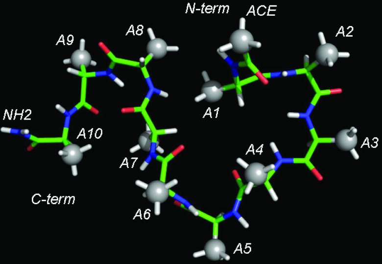
We apply the structure-based theory described above to polypeptide chains composed of alanine amino acid. The peptide is modeled in full atomic detail, as shown in Figure 2 for the number of residues N = 10, A10. The total solvation energy ΔG is split into two parts: electrostatic contribution ΔG_el and non-polar solvation ΔG_np. The electrostatic contribution together with the direct Coulomb interactions U_c are modeled as $U_c+\Delta G_{el}={\sum }_{i<j}\frac{q_i{q}_j}{\varepsilon \left(r_{ij}\right)r_{ij}}$, where q_i is the charge of particle i, r_ij is the distance between particles i and j, and ɛ(r) is the distance-dependent dielectric constant. The distance dependence in ɛ(r) accounts for the screening of charges at large separation and represents an approximate way to treat solvation free energy. This model meets our criterion of pair-wise additivity and is nowadays widely used in simulations of biological molecules.^{47, 71} Tests were conducted for several types of known^{72, 73} and newly designed distance dependences, in which the dielectric constant grew from around 1–3 at r ∼ 1 Å to 40–80 at r ∼ 10–15 Å. After parametrization, the results were found to be independent of the particular model. The results presented in the remainder of the paper were obtained for the linear model ɛ(r) = Dr,⁷³ where r is measured in Å and the proportionality constant D = 3 was determined from the maximum correlation between the solvation energy predicted by this model and the energy obtained by solving Poisson-Boltzmann (PB) equation for A10 peptide, as discussed in detail in Sec. 2D. The main purpose of the chosen electrostatics model is to separate out the long-range contribution from the total free energy.

Figure 2.

All-atom representation of alanine decapeptide (A10) considered in this work to extract effective inter-residue potentials. Gray spheres show the interaction sites for the non-polar potentials.

The non-polar contribution to the solvation energy is modeled with the help of effective potentials, $\Delta G_{np}={\sum }_{\alpha ,i<j}{u}_{\alpha }\left(r_{ij}\right)$, where the summation runs over all pairs of particles, indices i and j, and all types of contacts, index α. There are 9 types of contacts, 1–2 through 1–10, in a peptide with 10 residues. The non-polar solvation applies to all hydrophobic moieties present in the system. In the case of polyalanine these are the side chain groups centered on the C_β atoms, as shown in Figure 2. Additionally, the N-terminal acetyl (ACE) blocking group contains a hydrophobic methyl group, which is also added to the solvation model. Although this group is chemically identical to the side chains, geometrically it is distinct from them. Consequently, it has to be treated as a separate interaction site with its own set of potentials, u_0−i(r), where i runs from 1 to 10. In total, 19 different potentials are needed to describe the non-polar solvation of a decapeptide: 9 potentials are operating among side chains and 10 act between the N-terminal and the side chains.

Computational details

All simulations reported in this work were performed by GROMACS^{1, 74} molecular modeling package. The peptides were modeled with the optimized liquid state (OPLS/AA) force field⁵⁵ with neutralizing ACE and NH2 groups added at the carboxy and amino termini. All simulations were performed using replica exchange protocol⁷⁵ with the temperatures chosen equidistantly between two limiting values in inverse temperature. Replica exchanges were attempted every 250 time steps. The time step was set at 2 fs. The bonds involving hydrogen atoms in the protein were constrained according to the LINCS⁷⁶ algorithm.

Explicit solvent simulations were performed using TIP3P model⁷⁷ of water. The chemical bonds in water molecules were held constant by the SETTLE⁷⁸ algorithm. Nose-Hoover thermostat⁷⁹ with a 0.5 ps time constant was employed to maintain constant temperature. A single cut-off of 0.8 nm was used for the van der Waals interactions, with the neighbor lists updated every 10 time steps. Smooth-particle mesh Ewald (PME) method⁸⁰ was used to treat electrostatic interactions.

Implicit solvent simulations were performed using Langevin dynamics algorithm with the friction constant of 0.5 ps⁻¹. For the sake of computational efficiency, all non-bonded interactions, including the effective potentials, are assumed to be zero, or truncated at a cut-off distance Rc. In our simulations, Rc is set to 1.2 nm, which is large enough to include microscopic details of the effective interaction between two small hydrophobic molecules, such as the side chain of alanine, in water. Multiple trajectories and models were considered, as discussed in Sec. 3.

The electrostatic solvation energy was treated by distance-dependent (DD) dielectric constant model, ɛ(r) = Dr [Å], and the proportionality coefficient D was determined in the following way. One hundred peptide conformations, including the native state, were selected at random from the explicit solvent trajectory for A10. The electrostatic solvation energy was estimated for these states in the continuum approximation by solving the Poisson-Boltzmann equation in CHARMM.⁸¹ The solvation energy appropriate for the DD model was estimated as the difference between the total electrostatic energy in that model and the electrostatic energy in vacuum. To be consistent with the non-polar part of the solvation energy, a cut-off of 1.2 nm was employed. The correlation coefficient between PB and DD data was estimated as a function of D. Following a strong variation for small D < 1, the correlation coefficient reaches a plateau of about 0.91 for D > 3. A correlation of 1 indicates complete functional dependence between two variables. The slope of the linear fit between DD and PB results was also determined as a function of D, and was seen to decrease from around 0.9 for small D ∼ 1 to 0.2 for D > 5. The slope determines the electrostatic contribution to the free energy difference between two conformational states. As such, it should approach 1 for the accurate representation of the free energy landscape. We find that both properties, correlation coefficient and slope, can not reach values close to 1 for the same D. As a way of compromise, we chose D = 3 based on the condition that this value keeps the correlation coefficient high while maximizing the slope.

The length of the performed simulations was determined so as to ensure that the relevant pair distribution functions are converged. Two specific convergence tests were performed. First, the running average of g(r) was computed as a function of simulation time for each contact. The time when g(r) stopped changing noticeably, τ_c was identified as a tentative convergence time. Second, the simulation was continued for the amount of time τ_c and the resulting distribution function was compared with that obtained in the first half of the trajectory. If no differences were observed, the final g(r) was computed over the length of the entire trajectory, 2τ_c. Otherwise, the simulation was continued until the mentioned tests were passed. The number of conformations used for the computation of g(r) was varied to assess the sensitivity of the method to statistical errors. Lower numbers of conformations resulted in more noisy g(r) which in turn led to more noisy, but otherwise consistent, effective potentials. Severely undersampled data led to problems with spline interpolations and convergence of iterations and are not reported here. The summary of all performed simulations is shown in Table 1.

Table 1.

Summary of all simulations reported in this work.

Simulation	Simulation time (ns)	Temperatures (K)	Number of replicas	Size of the simulation box (nm)	Replica exchange probability (%)
Alanine decapeptide (A10) in explicit solvent	126	300–600	44	3.7	23–43
A10 in all implicit solvent models	80	250–600	12	8	28–52
Alanine polypeptide with 25 residues (A25) in explicit solvent	400	300–600	80	5.6	25–45
A25 using model M6/5	200	280–600	24	11.56	55–67
8 chains of peptide with 6 residues	1000	260–500	24	15	41–60
8 chains of peptide with 4 residues	1000	250–500	24	15	35–64

The secondary structure analysis of the multi-chain trajectories was performed using the protocol of Kabsch and Sander.⁸² What is referred to as β-structure and β-content in the discussion of the aggregation simulations is the amount of β-sheet and β-bridge structure added together. The reported probability is normalized so that it reaches the maximum value of 1 in the actual β-sheet conformation.

RESULTS

Implicit model with the maximum number of potentials

Derivation of effective potentials

Replica-exchange simulations in explicit solvent were conducted to obtain reference pair distribution functions g_R(r) for alanine decapeptide. These distribution functions were used to obtain 19 effective inter-residue potentials discussed in Sec. 2. The iterations were started from an initial state generated with the help of Lennard-Jones potentials that produce g(r) with maxima at approximately correct locations. After 30 iterations, the computed g(r)s stop changing visibly. Figure 3 shows the distribution functions for the nine inter-residue contacts 1–2 through 1–10 obtained in explicit and implicit solvent simulations at T = 300 K, the temperature for which the effective potentials were derived. The reference distribution functions are sufficiently converged, as can be seen from the panel of contact 1–6, which shows the data obtained for the first and the last 60 ns segments of the trajectory. The agreement between the explicit and implicit sets is remarkably good, with all the main features correctly reproduced for all contacts. Same quality agreement is seen for the ten distributions involving the ACE methyl group (data not shown), indicating that the employed model with 19 potentials is quantitatively correct as far as pair correlations among hydrophobic groups are concerned.

Figure 3.

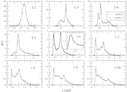
Pair distribution functions for different contacts as indicated in the graph, obtained in the explicit and implicit solvent simulations at T = 300 K. The two data sets are hardly distinguishable. An agreement of the same high quality is observed for the distribution functions involving the ACE methyl group. To illustrate the degree of convergence in the explicit solvent simulations, the panel for contact 1–6 shows the data for the first, broken line, and the last, dotted/broken line, 60 ns of the trajectory. Differences between the two parts are noticeable only upon magnification, as shown in the inset for the first maximum.

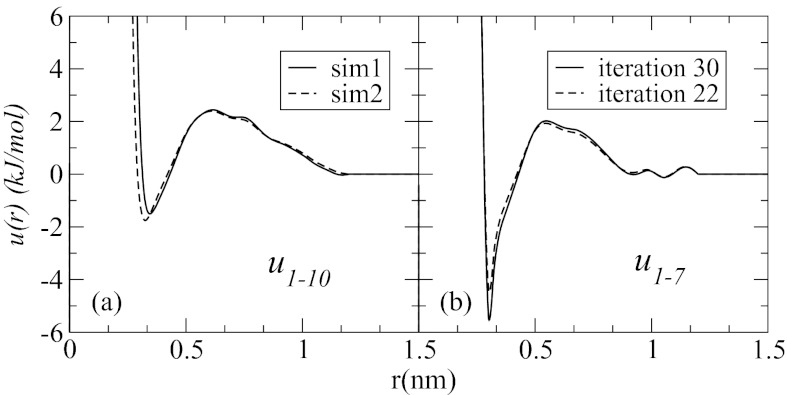
To test the convergence of the distribution functions, three independent sets of fitting simulations, sim1 through sim3, were performed. The simulations were started from different initial guesses of the effective potentials and took from 20 to 30 iterations to reach convergence (determined as the point where further iterations did not lead to improved distribution functions). All three simulations produced g(r)s that are indistinguishable to the eye, indicating that the solution is stable. The potentials obtained in these tests do not coincide exactly, however. As illustrated in Figure 4a, for u₁₋₁₀(r), different initial points produce slightly different potentials. As noted previously,^{61, 83} this is a consequence of the numerical nature of the applied procedure, since theoretically there is one-to-one correspondence between potentials and the corresponding distribution functions.⁶² It is seen that the region most affected by the numerical errors is short distance, r < 0.5 nm, where the pair distribution functions are subject to strong statistical noise. As a consequence, particle interaction energies in that region obtained from fitting are not reliable. In addition to different starting points, different iterations within one starting point also lead to noticeable differences in potentials, as shown in Figure 4b, for u₁₋₇(r), obtained in iterations 22 and 30 of sim3. Although small deviations are seen over the entire interaction range [0:1.2 nm], the most prominent differences are observed for small r, where the depth of the first minimum varies by ∼1 kJ/mol between iterations, or ∼20%. Since the distribution functions generated in the concerned simulations are indistinguishable, the applied structure-based procedure can determine effective interactions only up to a certain error.

Figure 4.

Examples of effective potentials obtained in two different fitting simulations, (a), and in one simulation at different iterations, (b). The potentials are determined up to a certain error due to the numerical nature of the applied procedure. The short-range part of the potentials is affected by the errors most.

Folding properties in explicit and implicit solvents

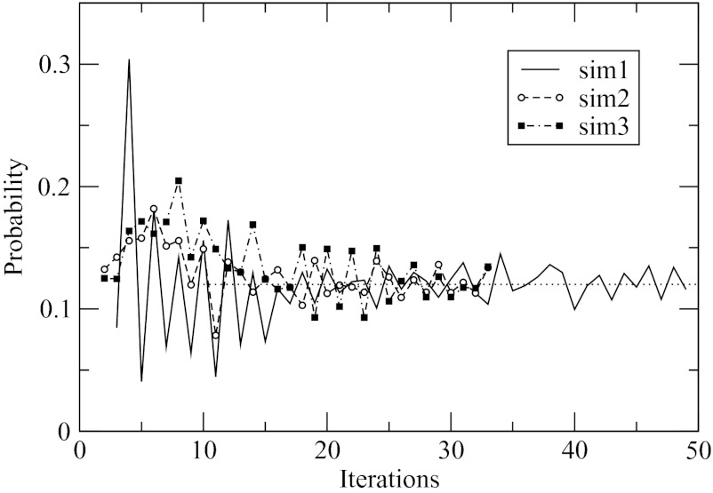
All conformations saved in the explicit solvent simulations were clustered according to C_α root mean square deviation (RMSD) among structures as a measure of similarity. A single α-helical conformation was observed as the most populated, or native, state. The distribution of RMSD computed for all structures with respect to the helical state showed a maximum at 0.1 nm and a minimum at 0.17 nm. The latter value was used as a cut-off to determine the population of the native state, leading to the estimate of 0.1. The same analysis was performed for the implicit solvent simulations. Clustering revealed the same native state for all three fitting runs, which was identical to the native state of the explicit solvent simulations. The progression of the population computed over successive iterations is shown in Figure 5. In all three runs, wide swings between 0.05 and 0.3 are seen in the initial 10 iterations, followed by small fluctuations. The magnitude of the fluctuations does not decay with time, as seen for sim1 continued for 50 iterations. This is a direct consequence of the numerical errors intrinsic in the applied procedure, which limit the accuracy with which the population can be determined. Figure 5 shows that the fluctuations occur between 0.1 and 0.14 with the average of 0.12, which is in a very good agreement with the value of 0.1 estimated in the explicit solvent simulations. Thus, even with the errors included, the implicit solvent model predicts essentially the same probability of the native state as the explicit solvent. This is quite encouraging given that the probability includes high-order correlations among particles, in addition to the two-particle correlations used in the derivation of the model.

Figure 5.

Population of the native state is determined in successive iterations of three independent fitting simulations. Convergence to the average value of 0.12 is seen in all three cases. The population observed in explicit solvent simulations is 0.1, in close agreement with the implicit solvent.

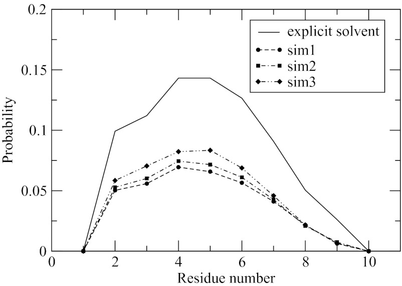
Since the peptide has a helical native state, it is instructive to analyze its folding in terms of a coil-helix transition. We use the formalism of Lifson and Roig (LR) for that purpose, which is a widely accepted helix-coil model.^{84, 85} Depending on the values of dihedral ϕ, ψ angles, residues in that model may remain in two states: helix or coil. We will assume that the helical residues are defined by −90° < ϕ < −30° and −77° < ψ < −17° while all other values indicate the coil state.⁸⁶ The statistical weight of the helical residues depends on whether they are part of helical segments. A helical residue is part of a helical segment if its immediate neighbors along the sequence, one residue preceding it and one residue following it, are also helical. This definition measures a correlated conversion of at least three residues into a helical state and precludes the terminal residues from being in helical segments. The helicity of each residue, or fraction of helix population, is defined as the probability to remain in a helical segment. Figure 6 shows this probability computed in the explicit and implicit solvent simulations. The implicit solvent data are consistent among all three simulations, with the individual probabilities differing by no more than 2 percentage points. The explicit solvent probabilities agree well with those of the implicit solvent at the qualitative level. The maximum at residues 4 and 5, a small shoulder at residue 2 and a gradual decrease of probabilities at the C-terminal, all these features are shared by the two sets of data. From quantitative perspective, the population in the implicit solvent is underestimated by 4–6 percentage points, depending on the residue.

Figure 6.

Probability of each residue to be in a helical segment is computed in this work in explicit and implicit solvent simulations. The implicit solvent model noticeably underestimates the “helicity.”

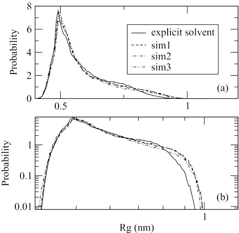
Figure 7 shows the distribution function of the radius of gyration over C_α atoms, Rg, obtained in implicit and explicit solvent simulations. The three implicit solvent runs again agree very well. In comparison with the explicit solvent, they reproduce correctly the main maximum at around 0.5 nm and the slowly decaying tail at large Rg. A small discrepancy is found in the tail region that is visible only on the log-log scale. As shown in Figure 7b, a shoulder in the explicit solvent curve at Rg = 0.75 nm is not reproduced in the implicit solvent data. Instead, a slightly larger population is seen for Rg > 0.8 nm. This effect is of small scale, however, as it affects an already insignificantly populated area of the conformational space.

Figure 7.

Probability distribution of the radius of gyration over C_α atoms in explicit and implicit solvent simulations, shown in linear, (a), and log-log, (b), scales. Small discrepancy between implicit and explicit solvent data are seen in panel (b) in the tail of the distribution function.

Transferable implicit solvent model

Model with a minimal number of potentials

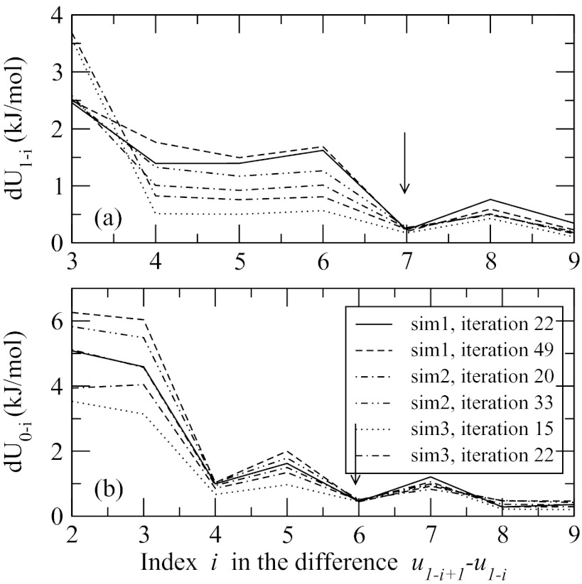
It is expected that not all effective potentials obtained for the decapeptide are unique. As argued in Sec. 2 based on general considerations, there should exist a maximum number K_max such that $u_{1-k}\left(r\right)=u_{1-K_{\max }}\left(r\right),k\ge K_{\max }$. To examine the change in u_1−k(r) over the contact number k, a quantity, $d{U}_{1-i}=\sqrt{\frac{{\int }_{r_{\min }}^{r_{\max }}{(u_{1-i+1}\left(r\right)-u_{1-i}\left(r\right))}^{2}dr}{r_{\max }-r_{\min }}},i=2,9,$ that compares how much the two potentials u_{1−i + 1}(r) and u_1−i(r) differ over the range [r_min, r_max] where they are defined, was computed. According to our arguments, dU_1−i should drop to zero at i = K_max. Figure 8 shows dU_1−i as a function of index i, panel (a), and an analogous property dU_0−i computed for the potentials acting between ACE and the side chains, panel (b). Multiple simulations/iterations are plotted to determine the reproducibility of the results. There is a significant scatter in the curves, especially for short-range neighbors with i = 2 and 3, that can be attributed to the numerical noise in the derivation of the potentials. A common trend in all plotted data is the rapid decline in both dU_1−i and dU_0−i after i = 4. Due to numerical reasons, these quantities never reach zero, which is expected. But for sufficiently long neighbors, indicated by arrows, the convergence to a plateau is observed. According to Figure 8, potentials for the side chains with contact number 7 and greater can be treated as identical. The same number for dU_0−i seems to be 6. The model with such properties has 6 unique potentials u_1−k(r), k = 2, 7, and 5 unique potentials u_0−k(r), k = 1, 5 (potential u₀₋₆(r) is set equal to u₁₋₇(r) in the long-range limit so it is not unique); in the remainder of the paper this model will be referred to as M6/5.

Figure 8.

Convergence of effective potentials for side chains, panel (a), and ACE and side chains, panel (b), to the limiting, density-independent shape in the limit of long-range contacts. Quantities dU_1−i and dU_0−i measure how much two potentials with contact numbers i + 1 and i differ. Arrows indicate where the dependence drops almost to zero. Multiple simulations and iterations are shown. The difference for the two shortest contacts, 1–2 and 1–3, for side chains and 0–1 and 0–2 for ACE group, is too large to be shown on the given scale.

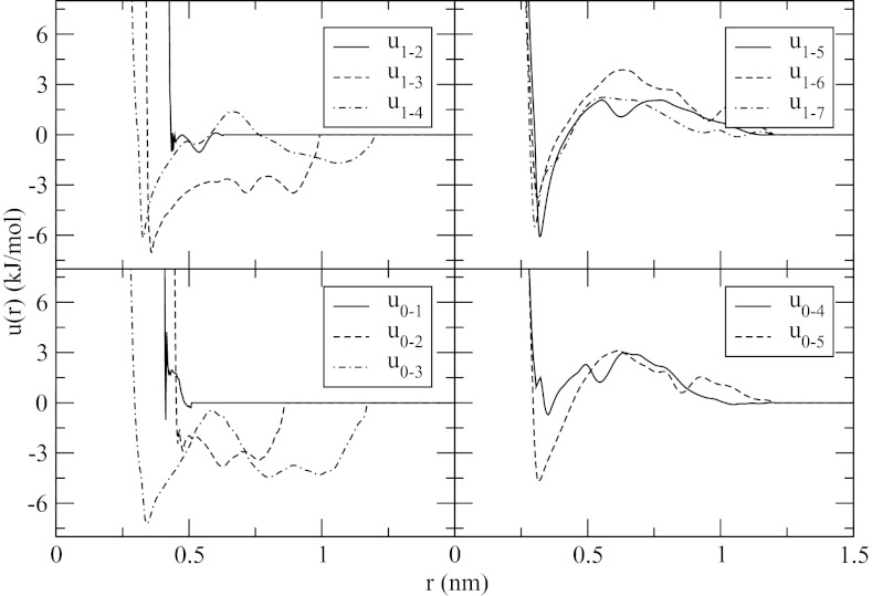
By design, M6/5 has 11 different types of inter-particle distances. Accordingly, 11 different potentials were re-derived from the explicit solvent trajectories assuming that the contacts 1–7 through 1–10 and 0–6 through 0–10 are treated as equivalent. The potentials, plotted in Figure 9, show strong dependence on the contact number for the nearest neighbors and the next nearest neighbors, u₁₋₂(r) − u₁₋₄(r) for the side chains and u₀₋₁(r) − u₀₋₃(r) for the side chains and ACE group. For some of these potentials, the distribution functions contain no data for r < Rc, prompting the truncation at a distance below the cut-off. Two potentials corresponding to the nearest-neighbor terms, u₀₋₁(r) and u₁₋₂(r), have spikes at short distances which are an artifact of the numerical tabulation.^{87, 88} The spikes have different appearances in different fitting simulations and do not affect the corresponding pair distribution functions. Starting at neighbors' three particles apart, u_1−k(r), k ⩾ 5, and u_0−k(r), k ⩾ 4, the potentials begin to develop common appearances. The most significant common features are the first minimum at r ∼ 0.33 nm and a broad maximum at r ∼ 0.65 nm. The minimum corresponds to close-contact configurations of the residues, while the maximum represents a barrier to contact formation/dissociation. The barrier is partly due to the solvation effects by water,⁸⁹ but it also contains averaged contributions from the peptide hydrophobic groups as well as the main chain atoms. At less than 3 kJ/mol, the desolvation barrier is too low to alter the dynamics of individual contact formation significantly.

Figure 9.

Effective potentials obtained for model M6/5.

Transferability tests

Figure 8 suggests that the peptide length of ten amino acid residues is sufficient to observe the convergence of the effective potentials to their limiting, long-range shape. As argued in Sec. 2, the converged potentials properly capture the density dependence, and therefore, should be transferable to peptides with larger numbers of residues. We test this prediction directly by investigating polyalanine chain with 25 residues (A25). In addition to model M6/5, we also consider models M4/3, M5/4, and M7/6, which are constructed in analogous way to M6/5 and contain 7, 9, and 13 unique potentials, respectively. Specifically, model M4/3 has 4 inter-side chain potentials and 3 potentials for the interactions of ACE with the side chains, model M5/4 has 5 inter-side chain potentials and 4 potentials for the interactions of ACE with the side chains, and model M7/6 has 7 inter-side chain potentials and 6 potentials for the interactions of ACE with the side chains. All these models produce indistinguishable pair distribution functions, when considered after a sufficiently large number of fitting iterations.

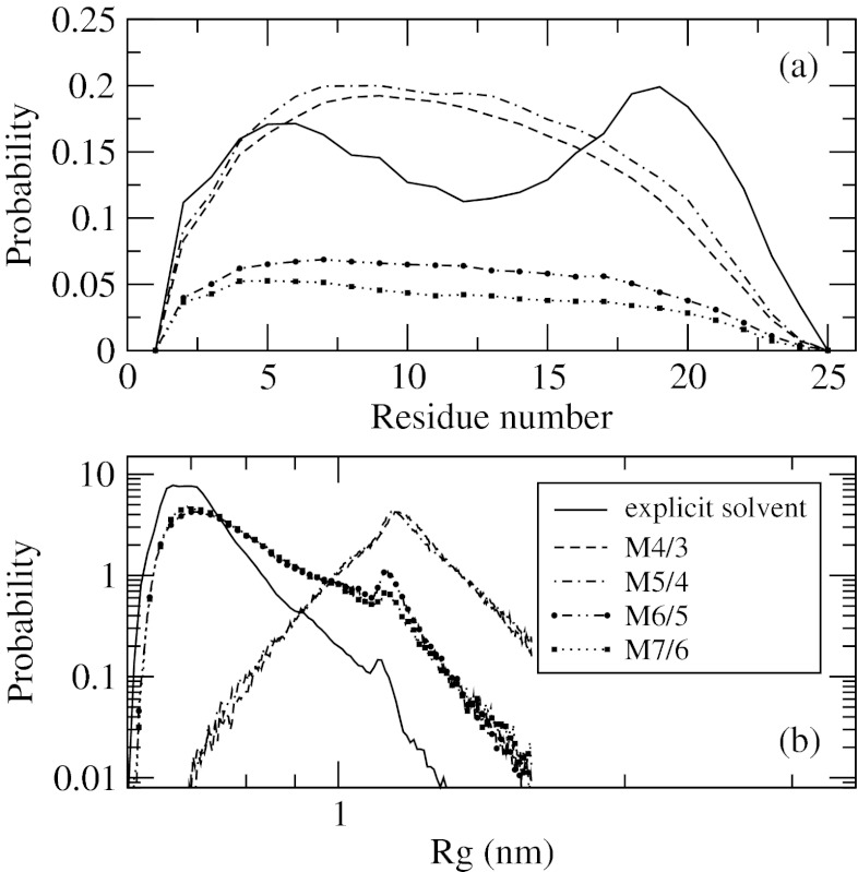
Explicit solvent simulations of A25 show that this peptide remains mostly a random coil, much like A10 discussed earlier. The helicity contents resolved for each residue are shown in Figure 10a. The level of structuring is seen to be the same as for A10, with probabilities reaching ∼0.15, except for residues 17–21, where they are slightly higher. Unlike A10, a minimum is observed for residues 12–13. The results of the implicit solvent models fall into two groups. The first group contains M4/3 and M5/4, and produces helicity in roughly good numerical agreement with the explicit solvent, with the exception of the minimum, which is not reproduced. The second group comprises M6/5 and M7/6, and displays lower helical probability overall but has a shape that better matches the explicit solvent results. Both models have a flat region between residues 5 and 17, with M7/6 displaying a shallow minimum. The implicit solvent should not be expected to perform better for A25 than it does for A10, for which it was originally derived. Therefore, taking into account the level of agreement between implicit and explicit solvents in A10, we conclude that the models in the first group, M4/3 and M5/4, are qualitatively wrong.

Figure 10.

Distribution of helicity across residues, panel (a), and distribution of the radius of gyration, panel (b), for polyalanine peptide with 25 residues. Panel (b) uses log-log scale for better visibility. Data of simulations in explicit solvent together with several implicit solvent models are shown. The models with fewer than 11 potentials are not transferable.

This conclusion is further reinforced in the analysis of the distribution function of the radius of gyration, P(Rg), shown in Figure 10b. It is seen that models with at least 11 potentials generate P(Rg) in good qualitative agreement with the explicit solvent. This includes the main maximum at Rg ∼ 0.7 nm, which is correctly predicted to have a majority population, and a small maximum at Rg ∼ 1.1 nm, which is seen to have a minority population. In contrast, M4/3 and M5/4 predict P(Rg) with only one, the second, maximum. Instead of populating collapsed coil states, these models predict expanded states, in direct contradiction to the explicit solvent simulations.

Both properties shown in Figure 10 indicate that the models with fewer than 11 effective potentials, M4/3 and M5/4, do not properly capture the density dependence in the context of polyalanine peptides, and thus, are not transferable. The non-transferability has quite dramatic consequences for the sampled conformational states, including the size of the peptide and its secondary structure. Models M6/5 and M7/6, on the other hand, produce results that are qualitatively correct, although the agreement with explicit solvent simulations is not as good as for A10. Both models are transferable in the sense that they provide a proper balance of different forces acting in the peptides across multiple length scales. The minimal transferable model suggested by our simulations is M6/5.

Application to multiple chains

Reversible aggregation of alanine tetra-peptide

To test the suitability of the minimal model for the studies of peptide self-assembly, two polyalanine systems with different number of residues N = 4 and 6 were considered. Eight polypeptide chains were modeled in a simulation box with the size of 15 nm, yielding a mM peptide concentration. The same concentration range was investigated in experimental studies of a similar alanine-rich peptide with a few charged residues added for solubility purposes.⁵⁶ The average distance between peptides at the chosen concentration is more than 40 Å, which is larger than the distance of 21 Å between neighbors 1 and 7 (the shortest fragment that yields transferable potentials) in the fully stretched peptide conformation. The polymer solution thus can be considered dilute, justifying the use of the inter-peptide potentials derived from the single-chain simulations.

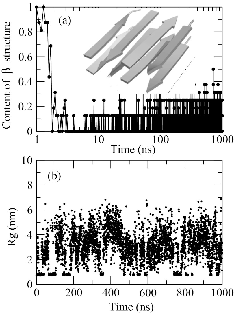
Both peptides, tetra-alanine and hexa-alanine, experience a transition into aggregated state at sufficiently low temperature. Figure 11 shows time evolution of the radius of gyration Rg over C_α atoms (computed after clustering the chains), and the total amount of β-structure (definition explained in Sec. 2) observed for N = 4 at T = 260 K in a trajectory started from two stacked in-register anti-parallel β-sheets, shown in the inset, as the initial conformation. The observation temperature is chosen below the transition temperature of both peptides. The initial β-structure disappears rapidly and irreversibly. After approximately 10 ns, the β-content drops from 100% to 20% and remains at that level throughout the remainder of the simulation (see Figure 11a). The loss of β-structure is not accompanied by the loss of aggregation, however. Figure 11b shows that the small Rg < 1 nm that initially corresponds to the β-sheet conformations persists well beyond the time point at which the β-structure melts. This indicates that aggregates of a new type are formed in the course of the simulation and that these aggregates are random-coil in structure. The aggregated states remain in dynamic equilibrium with the disaggregated conformations. The fact that the β-sheets convert into disordered aggregates and never reappear suggests that the latter represent a lower free energy state in our model. This conclusion is confirmed in two additional trajectories (data not shown): one started from a random-coil disaggregated state and the other from an in-register, parallel β-sheet conformation, both of which lead to the disordered aggregates as the most populated species. Collectively, our simulations indicate that the tetra-peptide aggregates mostly into random-coil states.

Figure 11.

Time traces obtained in the simulation of 8 tetra-alanine chains that was started from a stacked anti-parallel β-sheet (shown in the inset) as the initial conformation. Panel (a) shows the amount of β-structure as a function of time (note the log scale of the x axis). The initial β-sheet disappears in the first 10 ns of the simulation and never re-emerges. Panel (b) shows radius of gyration Rg computed over C_α atoms. Aggregated conformations, Rg < 1 nm, are in equilibrium with the disaggregated states, Rg > 1 nm. After the first 10 ns, only non-β-sheet aggregates remain.

β propensity of aggregates increases with the length of the peptide chain

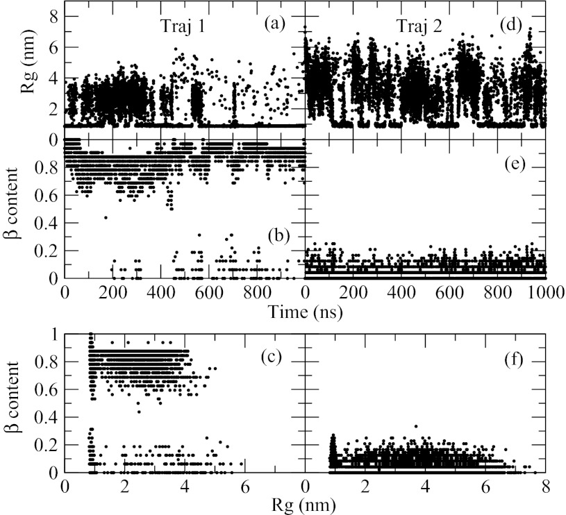
Figure 12 shows the same quantities, generated at the same temperature and peptide concentration, as Figure 11 but for N = 6. In addition to the trajectory started from a β-sheet, panels (a), (b), and (c), the data obtained for the trajectory started from a disaggregated random-coil conformation, panels (d), (e), and (f), are also shown. The behavior of the radius of gyration (Figure 12a, 12d) demonstrates that the system is mostly aggregated in both trajectories at the chosen temperature. Comparison with Figure 11b clearly shows that the peptide with six residues aggregates more abundantly than the peptide with four residues. The β-content in the first trajectory, Figure 12b, drops from 100% to about 80% in the first few nanoseconds but remains little changed in the remainder of the simulation. At approximately 200 ns, conformations with a low ∼10% population of β-structure begin to appear. The second trajectory, Figure 12e, produces only non-β conformations. Figure 12c, depicting 2D map of the β-content against Rg, shows that the non-β conformations sampled in the first trajectory are both aggregated, small Rg, and disaggregated, large Rg. Conformations rich in β-structure can also be either small, complete β-sheet, or large, Rg > 2 nm, corresponding to a β-sheet with one dissociated β-strand. The second trajectory, Figure 12f, samples both compact and expanded states but without β-structure. The disordered aggregated conformations, therefore, are seen in both trajectories but constitute a majority only in the second trajectory, while in the first trajectory their population is low. To determine which of the two states, β-sheet or disordered aggregates, constitutes the true free energy minimum, we conducted a third test simulation in which half of all replicas were assigned β-sheet conformation, while the other half were assumed to be aggregated random coils. This setup permits the two conformations to compete directly with one another, thus allowing us to determine the lower free energy state. A population shift toward β-sheet was observed in the test, indicating that β-sheet is the more stable structure. Thus, the peptide with 6 amino acids aggregates mostly into β-sheet states at low temperature. This is in contrast to the tetra-peptide, which aggregates predominantly into disordered conformations. The lack of β-sheet formation in the second trajectory (Figure 12e) indicates that this structure is kinetically hindered. Slow nucleation is not uncommon in the fibril formation of many peptides.⁹⁰ Primary structure composed of only one amino acid, like in the studied system, is known to induce frustration^{91, 92} in the free energy landscape. The frustration is most likely the main reason for the observed slow relaxation.

Figure 12.

Time traces of two trajectories generated for the system composed of 8 chains of alanine hexa-peptide. (Panels (a)–(c)) Trajectory 1 corresponds to anti-parallel β-sheet initial conformation. (Panels (d)–(f)) Trajectory 2 shows the data for a disaggregated, random-coil initial conformation. Radius of gyration, panels (a) and (d), and the amount of β-structure, panels (b) and (e), are shown as a function of time in the two trajectories. 2D plots of these two quantities are shown in panels (c) and (f).

The aggregation behavior observed for our tetra- and hexa-peptide models is consistent with the recent experimental studies of alanine-rich peptides (with a few charged residues added for solubility reasons).^{40, 56} Like the experiments, our simulations find that polyalanines aggregate into β-sheet structure more readily with the growing length of the peptide chain. The length dependence is an important characteristic of the aggregation process and it is clear that the proposed model is able to capture it.

CONCLUSIONS

In this paper, we introduced an approach to conduct simulations of large proteins and protein complexes in atomic detail using pair-wise decomposition of the solvation free energy. The strategy derives effective potentials that mimic the presence of solvent using as input the pair-distribution functions of amino acid residues generated in explicit solvent simulations. We showed that our approach correctly reproduces folding of a small all-alanine peptide with 10 amino acid residues. The potentials that result from the matching of pair-distribution functions represent free energy and thus depend on the thermodynamic properties of the studied system such as temperature and density. The variation with the density is strong for the nearest neighbors along the chain but vanishes for larger separation among the residues. We showed that a segment comprised of 7 residues, and characterized by 11 different potentials, constitutes the minimal model capable of capturing the correct density dependence. Simulations of a longer alanine peptide with 25 residues lead to qualitatively correct conclusions compared to explicit solvent data, proving that the model is transferable. When tested on systems with multiple chains, the model predicts that longer alanine-based peptides self-assemble into β-sheet structures reminiscent of amyloid fibrils more readily than do the shorter ones. This result is again qualitatively correct compared to experiment. Our tests demonstrate that the derived potentials can be used in computational studies of peptide aggregation to routinely generate microsecond replica-exchange trajectories for atomically accurate models, a speed that compares very favorably to that of similar recent studies conducted in explicit solvent over nanosecond time scale.^{8, 93}

While the introduced model produces qualitatively correct results for the native state, there are some differences with the explicit solvent in the broader folding landscape, in particular, the distribution of the helicity along the chain and the radius of gyration. The discrepancies are due to the various approximations inherent in the model, which need to be critically assessed in order to better understand the model's limitations and in order to formulate strategies for improvement. We note the following features and assumptions upon which the model is built that may negatively affect its accuracy:

1. The non-polar energy is applied to selected degrees of freedom only, C_β atoms of the side chains. This is an approximation, which could have adverse effects if overall peptide conformation was able to change substantially for the fixed configuration of the side chains (and the methyl group of ACE). Given the rigid geometry of the peptide bond and the fact that there is only one heavy atom in the side chain, this seems unlikely.

2. The neglect of the boundary effect in inter-residue potentials, or u_i,j = u_j−i approximation. This effect is local, specific to each residue, and thus cannot explain why the implicit solvent underestimates the helicity globally, for each residue of the chain.

3. Truncation of the effective potentials. The truncation distance of 1.2 nm is sufficiently long to include all important features in the potential of mean force between two hydrophobic moieties in water. It is thus not expected to cause artifacts.

4. The solvation free energy is assumed to be pair-wise additive. At the level of pair correlations, this assumption is correct, ensured by the use of the procedure relying on g(r). There is no guarantee, however, that this approximation describes fully multi-body correlations. Using helicity as an example, to be in a helical state, a particular residue requires that two adjacent residues are helical as well. Accordingly, helicity measures a correlated probability among at least three particles. Same arguments apply to the radius of gyration. Since these probabilities are not well reproduced by the implicit solvent, it is possible that the cause of the discrepancy is the pair approximation. We note that some multi-body contributions are present in the model through the density dependence of the potentials. However, they may not be enough to reproduce multi-particle correlations with quantitative accuracy. This issue needs to be further researched in direct estimates of the multi-particle potentials and their contribution to the conformational statistics.

The limitations discussed above in reference to the folding statistics also apply to simulations of protein aggregation. Here as well, the contribution of multi-body potentials is the most difficult one to assess. Like in any atomistic force-field with fixed charges, the multi-body effects in our model may turn out to be important for certain aspects of the aggregation process. Researching these effects, however, will be more challenging than in folding simulations. Unlike folding, ab initio simulations of complete aggregation reaction in explicit solvent are currently out of reach and will remain so in the foreseeable future, even for relatively small systems and even with the help of various accelerated sampling techniques. The progress in this area, therefore, will have to be guided mostly by comparison with experiment.

References

- Van der Spoel D. et al. , J. Comput. Chem. 26, 1701 (2005). 10.1002/jcc.20291 [DOI] [PubMed] [Google Scholar]
- van Gunsteren W. F. and Dolenc J., Biochem. Soc. Trans. 36, 11 (2008). 10.1042/BST0360011 [DOI] [PubMed] [Google Scholar]
- Hartl F. U., Bracher A., and Hayer-Hartl M., Nature (London) 475, 324 (2011). 10.1038/nature10317 [DOI] [PubMed] [Google Scholar]
- Elcock A. H., Sept D., and McCammon J. A., J. Phys. Chem. B 105, 1504 (2001). 10.1021/jp003602d [DOI] [Google Scholar]
- Eisenberg D. et al. , Acc. Chem. Res. 39, 568 (2006). 10.1021/ar0500618 [DOI] [PMC free article] [PubMed] [Google Scholar]
- Tarus B., Straub J. E., and Thirumalai D., J. Mol. Biol. 345, 1141 (2005). 10.1016/j.jmb.2004.11.022 [DOI] [PubMed] [Google Scholar]
- Gnanakaran S., Nussinov R., and Garcia A. E., J. Am. Chem. Soc. 128, 2158 (2006). 10.1021/ja0548337 [DOI] [PubMed] [Google Scholar]
- Rohrig U. F. et al. , Biophys. J. 91, 3217 (2006). 10.1529/biophysj.106.088542 [DOI] [PMC free article] [PubMed] [Google Scholar]
- Nguyen H. D. and Hall C. K., Proc. Natl. Acad. Sci. U.S.A. 101, 16180 (2004). 10.1073/pnas.0407273101 [DOI] [PMC free article] [PubMed] [Google Scholar]
- Santini S., Mousseau N., and Derreumaux P., J. Am. Chem. Soc. 126, 11509 (2004). 10.1021/ja047286i [DOI] [PubMed] [Google Scholar]
- Morriss-Andrews A., Bellesia G., and Shea J. E., J. Chem. Phys. 135, 085102 (2011). 10.1063/1.3624929 [DOI] [PubMed] [Google Scholar]
- Honeycutt J. D. and Thirumalai D., Biopolymers 32, 695 (1992). 10.1002/bip.360320610 [DOI] [PubMed] [Google Scholar]
- Urbanc B. et al. , Biophys. J. 87, 2310 (2004). 10.1529/biophysj.104.040980 [DOI] [PMC free article] [PubMed] [Google Scholar]
- Tsiavaliaris G. et al. , EMBO Rep. 3, 1099 (2002). 10.1093/embo-reports/kvf214 [DOI] [PMC free article] [PubMed] [Google Scholar]
- Bitan G., Vollers S. S., and Teplow D. B., J. Biol. Chem. 278, 34882 (2003). 10.1074/jbc.M300825200 [DOI] [PubMed] [Google Scholar]
- Roux B. and Simonson T., Biophys. Chem. 78, 1 (1999). 10.1016/S0301-4622(98)00226-9 [DOI] [PubMed] [Google Scholar]
- Okur A. and Simmerling C., in Annual Reports in Computational Chemistry, edited by David C. S. (Elsevier, 2006), pp. 97. [Google Scholar]
- Bashford D. and Case D. A., Annu. Rev. Phys. Chem. 51, 129 (2000). 10.1146/annurev.physchem.51.1.129 [DOI] [PubMed] [Google Scholar]
- Cramer C. J. and Truhlar D. G., Chem. Rev. 99, 2161 (1999). 10.1021/cr960149m [DOI] [PubMed] [Google Scholar]
- Israelachvili J. and Pashley R., Nature (London) 300, 341 (1982). 10.1038/300341a0 [DOI] [PubMed] [Google Scholar]
- Ben-Naim A., J. Chem. Phys. 90, 7412 (1989). 10.1063/1.456221 [DOI] [Google Scholar]
- Ooi T. et al. , Proc. Natl. Acad. Sci. U.S.A. 84, 3086 (1987). 10.1073/pnas.84.10.3086 [DOI] [PMC free article] [PubMed] [Google Scholar]
- Varilly P., Patel A. J., and Chandler D., J. Chem. Phys. 134, 074109 (2011). 10.1063/1.3532939 [DOI] [PMC free article] [PubMed] [Google Scholar]
- Sharp K. A. et al. , Science 252, 106 (1991). 10.1126/science.2011744 [DOI] [PubMed] [Google Scholar]
- Baumketner A. and Nesmelov Y. E., Protein Sci. 20, 2013 (2011). 10.1002/pro.737 [DOI] [PMC free article] [PubMed] [Google Scholar]
- Dill K. A. et al. , Annu. Rev. Biophys. 37, 289 (2008). 10.1146/annurev.biophys.37.092707.153558 [DOI] [PMC free article] [PubMed] [Google Scholar]
- Allen M. P. and Tildesley D. J., Computer Simulations of Liquids (Oxford University Press, Oxford, 1987). [Google Scholar]
- Frenkel D. and Smit B., Understanding Molecular Simulation (Academic, San Diego, 2002). [Google Scholar]
- Lyubartsev A. P. and Laaksonen A., Phys. Rev. E 55, 5689 (1997). 10.1103/PhysRevE.55.5689 [DOI] [Google Scholar]
- Lyubartsev A. P. and Nordenskiold L., J. Phys. Chem. B 101, 4335 (1997). 10.1021/jp963982w [DOI] [Google Scholar]
- Villa A., Peter C., and van der Vegt N. F. A., Phys. Chem. Chem. Phys. 11, 2077 (2009). 10.1039/b818144f [DOI] [PubMed] [Google Scholar]
- Villa A., van der Vegt N. F. A., and Peter C., Phys. Chem. Chem. Phys. 11, 2068 (2009). 10.1039/b818146m [DOI] [PubMed] [Google Scholar]
- Lyubartsev A. P., Eur. Biophys. J. 35, 53 (2005). 10.1007/s00249-005-0005-y [DOI] [PubMed] [Google Scholar]
- Akkermans R. L. C. and Briels W. J., J. Chem. Phys. 114, 1020 (2001). 10.1063/1.1330744 [DOI] [Google Scholar]
- Fukunaga H., Takimoto J., and Doi M., J. Chem. Phys. 116, 8183 (2002). 10.1063/1.1469609 [DOI] [Google Scholar]
- Ashbaugh H. S. et al. , J. Chem. Phys. 122, 104908 (2005). 10.1063/1.1861455 [DOI] [PubMed] [Google Scholar]
- Reith D., Putz M., and Muller-Plathe F., J. Comput. Chem. 24, 1624 (2003). 10.1002/jcc.10307 [DOI] [PubMed] [Google Scholar]
- Allen E. C. and Rutledge G. C., J. Chem. Phys. 130, 204903 (2009). 10.1063/1.3139025 [DOI] [PubMed] [Google Scholar]
- Faux N. G. et al. , Genome Res. 15, 537 (2005). 10.1101/gr.3096505 [DOI] [PMC free article] [PubMed] [Google Scholar]
- Bernacki J. P. and Murphy R. M., Biochemistry 50, 9200 (2011). 10.1021/bi201155g [DOI] [PubMed] [Google Scholar]
- Nguyen H. D. and Hall C. K., J. Am. Chem. Soc. 128, 1890 (2006). 10.1021/ja0539140 [DOI] [PMC free article] [PubMed] [Google Scholar]
- Cheon M., Chang I., and Hall C. K., Biophys. J. 101, 2493 (2011). 10.1016/j.bpj.2011.08.042 [DOI] [PMC free article] [PubMed] [Google Scholar]
- Pellarin R., Guarnera E., and Caflisch A., J. Mol. Biol. 374, 917 (2007). 10.1016/j.jmb.2007.09.090 [DOI] [PubMed] [Google Scholar]
- Wei G. H., Mousseau N., and Derreumaux P., Biophys. J. 87, 3648 (2004). 10.1529/biophysj.104.047688 [DOI] [PMC free article] [PubMed] [Google Scholar]
- Bellesia G. and Shea J. E., J. Chem. Phys. 130, 145103 (2009). 10.1063/1.3108461 [DOI] [PubMed] [Google Scholar]
- Paci E. et al. , J. Mol. Biol. 340, 555 (2004). 10.1016/j.jmb.2004.05.009 [DOI] [PubMed] [Google Scholar]
- Cecchini M. et al. , J. Mol. Biol. 357, 1306 (2006). 10.1016/j.jmb.2006.01.009 [DOI] [PubMed] [Google Scholar]
- Cecchini M. et al. , J. Chem. Phys. 121, 10748 (2004). 10.1063/1.1809588 [DOI] [PubMed] [Google Scholar]
- Gsponer J., Haberthur U., and Caflisch A., Proc. Natl. Acad. Sci. U.S.A. 100, 5154 (2003). 10.1073/pnas.0835307100 [DOI] [PMC free article] [PubMed] [Google Scholar]
- Irback A. and Mitternacht S., Proteins: Struct., Funct., Bioinf. 71, 207 (2008). 10.1002/prot.21682 [DOI] [PubMed] [Google Scholar]
- Li D. W. et al. , PLOS Comput. Biol. 4, e1000238 (2008). 10.1371/journal.pcbi.1000238 [DOI] [PMC free article] [PubMed] [Google Scholar]
- Cheon M. et al. , PLOS Comput. Biol. 3, e173 (2007). 10.1371/journal.pcbi.0030173 [DOI] [PMC free article] [PubMed] [Google Scholar]
- Walsh D. M. et al. , J. Biol. Chem. 272, 22364 (1997). 10.1074/jbc.272.35.22364 [DOI] [PubMed] [Google Scholar]
- Walsh D. M. et al. , J. Biol. Chem. 274, 25945 (1999). 10.1074/jbc.274.36.25945 [DOI] [PubMed] [Google Scholar]
- Kaminski G. A. et al. , J. Phys. Chem. B 105, 6474 (2001). 10.1021/jp003919d [DOI] [Google Scholar]
- Blondelle S. E. et al. , Biochemistry 36, 8393 (1997). 10.1021/bi963015b [DOI] [PubMed] [Google Scholar]
- Praprotnik M., Delle Site L., and Kremer K., Annu. Rev. Phys. Chem. 59, 545 (2008). 10.1146/annurev.physchem.59.032607.093707 [DOI] [PubMed] [Google Scholar]
- Schommers W., Phys. Lett. A 43, 157 (1973). 10.1016/0375-9601(73)90591-4 [DOI] [Google Scholar]
- Schommers W., Phys. Rev. A 28, 3599 (1983). 10.1103/PhysRevA.28.3599 [DOI] [Google Scholar]
- Levesque D., Weis J. J., and Reatto L., Phys. Rev. Lett. 54, 451 (1985). 10.1103/PhysRevLett.54.451 [DOI] [PubMed] [Google Scholar]
- Soper A. K., Chem. Phys. 202, 295 (1996). 10.1016/0301-0104(95)00357-6 [DOI] [Google Scholar]
- Henderson R. L., Phys. Lett. A 49, 197 (1974). 10.1016/0375-9601(74)90847-0 [DOI] [Google Scholar]
- Lyubartsev A. P. and Laaksonen A., Phys. Rev. E 52, 3730 (1995). 10.1103/PhysRevE.52.3730 [DOI] [PubMed] [Google Scholar]
- Ruhle V. et al. , J. Chem. Theory Comput. 5, 3211 (2009). 10.1021/ct900369w [DOI] [PubMed] [Google Scholar]
- Ercolessi F. and Adams J. B., Europhys. Lett. 26, 583 (1994). 10.1209/0295-5075/26/8/005 [DOI] [Google Scholar]
- Izvekov S. and Voth G. A., J. Phys. Chem. B 109, 2469 (2005). 10.1021/jp044629q [DOI] [PubMed] [Google Scholar]
- Zhou J. et al. , Biophys. J. 92, 4289 (2007). 10.1529/biophysj.106.094425 [DOI] [PMC free article] [PubMed] [Google Scholar]
- Liu P., Izvekov S., and Voth G. A., J. Phys. Chem. B 111, 11566 (2007). 10.1021/jp0721494 [DOI] [PubMed] [Google Scholar]
- Izvekov S. and Voth G. A., J. Phys. Chem. B 113, 4443 (2009). 10.1021/jp810440c [DOI] [PMC free article] [PubMed] [Google Scholar]
- De Gennes P. G., Scaling Concepts in Polymer Physics (Cornell University Press, New York, 1979). [Google Scholar]
- Kim S., Takeda T., and Klimov D. K., Biophys. J. 99, 1949 (2010). 10.1016/j.bpj.2010.07.008 [DOI] [PMC free article] [PubMed] [Google Scholar]
- Ramstein J. and Lavery R., Proc. Natl. Acad. Sci. U.S.A. 85, 7231 (1988). 10.1073/pnas.85.19.7231 [DOI] [PMC free article] [PubMed] [Google Scholar]
- Guenot J. and Kollman P. A., Protein Sci. 1, 1185 (1992). 10.1002/pro.5560010912 [DOI] [PMC free article] [PubMed] [Google Scholar]
- Hess B. et al. , J. Chem. Theory Comput. 4, 435 (2008). 10.1021/ct700301q [DOI] [PubMed] [Google Scholar]
- Sugita Y. and Okamoto Y., Chem. Phys. Lett. 314, 141 (1999). 10.1016/S0009-2614(99)01123-9 [DOI] [Google Scholar]
- Hess B. et al. , J. Comput. Chem. 18, 1463 (1997). [DOI] [Google Scholar]
- Jorgensen W. L. et al. , J. Chem. Phys. 79, 926 (1983). 10.1063/1.445869 [DOI] [Google Scholar]
- Miyamoto S. and Kollman P. A., J. Comput. Chem. 13, 952 (1992). 10.1002/jcc.540130805 [DOI] [Google Scholar]
- Nose S., Prog. Theor. Phys. Suppl. 103, 1 (1991). 10.1143/PTPS.103.1 [DOI] [Google Scholar]
- Essmann U. et al. , J. Chem. Phys. 103, 8577 (1995). 10.1063/1.470117 [DOI] [Google Scholar]
- Brooks B. R. et al. , J. Comput. Chem. 4, 187 (1983). 10.1002/jcc.540040211 [DOI] [Google Scholar]
- Kabsch W. and Sander C., Biopolymers 22, 2577 (1983). 10.1002/bip.360221211 [DOI] [PubMed] [Google Scholar]
- Almarza N. G. and Lomba E., Phys. Rev. E 68, 011202 (2003). 10.1103/PhysRevE.68.011202 [DOI] [PubMed] [Google Scholar]
- Poland D. and Scheraga H. A., Theory of Helix-Coil Transitions in Biopolymers, 1st ed. (Academic, New York, 1970). [Google Scholar]
- Best R. B. and Hummer G., J. Phys. Chem. B 113, 9004 (2009). 10.1021/jp901540t [DOI] [PMC free article] [PubMed] [Google Scholar]
- Gnanakaran S. and Garcia A. E., J. Phys. Chem. B 107, 12555 (2003). 10.1021/jp0359079 [DOI] [Google Scholar]
- Sippl M. J., J. Mol. Biol. 213, 859 (1990). 10.1016/S0022-2836(05)80269-4 [DOI] [PubMed] [Google Scholar]
- Jain S., Garde S., and Kumar S. K., Ind. Eng. Chem. Res. 45, 5614 (2006). 10.1021/ie060042h [DOI] [Google Scholar]
- Cheung M. S., Garcia A. E., and Onuchic J. N., Proc. Natl. Acad. Sci. U.S.A. 99, 685 (2002). 10.1073/pnas.022387699 [DOI] [PMC free article] [PubMed] [Google Scholar]
- Chiti F. et al. , Proc. Natl. Acad. Sci. U.S.A. 99, 16419 (2002). 10.1073/pnas.212527999 [DOI] [PMC free article] [PubMed] [Google Scholar]
- Shakhnovich E. I. and Gutin A. M., Biophys. Chem. 34, 187 (1989). 10.1016/0301-4622(89)80058-4 [DOI] [PubMed] [Google Scholar]
- Pande V. S., Grosberg A. Y., and Tanaka T., Rev. Mod. Phys. 72, 259 (2000). 10.1103/RevModPhys.72.259 [DOI] [Google Scholar]
- Singh G. et al. , J. Phys. Chem. B 113, 9863 (2009). 10.1021/jp901144v [DOI] [PubMed] [Google Scholar]