Effect of the 2010 Chilean Earthquake on Posttraumatic Stress Reducing Sensitivity to Unmeasured Bias Through Study Design

Abstract

In 2010, a magnitude 8.8 earthquake hit Chile, devastating parts of the country. Having just completed its national socioeconomic survey, the Chilean government reinterviewed a subsample of respondents, creating unusual longitudinal data about the same persons before and after a major disaster. The follow-up evaluated posttraumatic stress symptoms (PTSS) using Davidson’s Trauma Scale. We use these data with two goals in mind. Most studies of PTSS after disasters rely on recall to characterize the state of affairs before the disaster. We are able to use prospective data on preexposure conditions, free of recall bias, to study the effects of the earthquake. Second, we illustrate recent developments in statistical methodology for the design and analysis of observational studies. In particular, we use new and recent methods for multivariate matching to control 46 covariates that describe demographic variables, housing quality, wealth, health, and health insurance before the earthquake. We use the statistical theory of design sensitivity to select a study design with findings expected to be insensitive to small or moderate biases from failure to control some unmeasured covariate. PTSS were dramatically but unevenly elevated among residents of strongly shaken areas of Chile when compared with similar persons in largely untouched parts of the country. In 96% of exposed-control pairs exhibiting substantial PTSS, it was the exposed person who experienced stronger symptoms (95% confidence interval = 0.91–1.00).

At 3:34 on Saturday morning, 27 February 2010, an earthquake of magnitude 8.8 struck in the Pacific Ocean, 65 miles west of Concepción, Chile. This was the planet’s sixth most severe earthquake since 1900.¹ The quake and tsunami caused more than $30 billion in damages, damaging or destroying 370,000 houses, 4013 schools, and 79 hospitals.¹ More than 500 people were crushed, drowned, or burned to death by fires.¹

Posttraumatic stress symptoms (PTSS) are often reported after earthquakes.^2,3 The literature suggests that the psychological effects of trauma vary from one person to another, possibly because of differing resilience to psychological stress.^4,5 Also, two persons may experience the same event but experience different traumas, such as physical injury or loss of a loved one, and may be differently affected by displacement, loss of income, and destruction of property.^6,7 Because most people who experience injury or loss of income do not develop frank posttraumatic stress disorder, heterogeneous experiences explain only part of heterogeneous symptoms. A limitation of many studies is that, because an earthquake or similar disaster is not anticipated, investigators most usually rely on retrospective recall of key variables, such as intensity of exposure and conditions before exposure. A person in distress after an earthquake may recall exposure to the earthquake as more severe than someone not in distress,^8,9 or may recall conditions before the earthquake differently. If distress distorts memory, it may consequently distort associations between current status and recalled exposure adjusting for recalled preexposure status. The current investigation addresses these difficulties by using prospectively recorded conditions before the earthquake, and objective geologic measures of ground shaking.

Natural disasters strike without purpose or deliberate target, but they are less equitable than randomized experiments. Low-income residential areas may be more often found along fault lines, low-income homes may be constructed of poorer materials less resistant to earthquake damage, and poor health or limited financial resources may limit ability to respond and recover after an earthquake has struck.

Chile’s earthquake provides a unique opportunity because, shortly before the earthquake, Chile’s Ministry of Planning and Cooperation had completed its national socioeconomic survey (CASEN). Shortly after the earthquake, they reinterviewed a subsample of the original respondents. It is unusual to have detailed data on the same persons for a large sample before and after a major disaster.

We use these data not just to assess the effects of the quake, but also to illustrate recent developments in statistics concerning the planning of observational studies to reduce sensitivity to unmeasured biases. A sensitivity analysis quantifies the magnitude of unmeasured bias that would need to be present to materially alter the conclusions of the study.^10–15 Studies vary substantially in their sensitivity to unmeasured biases—a fact that is not revealed by the magnitude of a P value computed assuming that there is no bias.^16–19 Like statistical power, design sensitivity anticipates the outcome of a sensitivity analysis when the data are generated by a particular design and analyzed by particular methods. Once quantified, study designs and methods of analysis are seen to vary substantially in their tendency to yield results sensitive to unmeasured biases, a fact that is not revealed by power calculations performed assuming that there is no bias.^16–19

The specific tactics used here to reduce sensitivity to unmeasured biases include the following:

• Prospective natural experiment with extensive covariates. One seeks a situation in which the treatment is inflicted on one person and withheld from another in a somewhat haphazard fashion, without deliberate purpose, and in which many relevant pretreatment covariates are measured prospectively. In such a situation, one does not anticipate large unmeasured biases—in part because large biases of all kinds are not anticipated and in part because many potential sources of bias are measured. As noted above, the Chilean earthquake is unusual among disaster studies in satisfying the second condition.

• Extreme exposures, rather than a continuum including minor exposures. One seeks to compare a treated and control group that experience very different exposures to the treatment.^16–18 For this reason, we compare severely shaken and largely untouched regions of Chile.

• Methods tailored to anticipated patterns of response. The general principle is that if one anticipates a specific pattern of treatment effects, one uses methods that can detect this specific pattern. In the specific case considered here, we anticipate severe PTSS in some but far from all persons severely shaken by the earthquake. Using methods designed to detect such a response pattern will reduce sensitivity to bias if the anticipated pattern does, in fact, occur.^17–21 If one represented severe versus negligible exposure by a term in a model, such as indicator variable or a continuous measure of ground shaking in a regression, the model would estimate a typical effect with a magnitude that would greatly understate the effects of the trauma on some persons, and by understating the true magnitude of effect, would overstate the sensitivity to unmeasured biases.

Investigating sensitivity to unmeasured covariates is facilitated by the use of simple, transparent methods to control for measured covariates, such as multivariate matching.^17,22 Multivariate matching compares matched treated and control groups that look comparable before treatment with respect to many measured covariates. Whether groups look comparable in measured covariates is a fact in the data that can be settled unambiguously before entertaining the inevitably more contentious and uncertain issues involving unmeasured covariates. When these tasks are merged—when adjustments for observed covariates are merged with sensitivity analysis for unobserved covariates—it can be difficult to determine the extent to which either task has been completed successfully (17, Chapter 6).

Our analysis uses recent techniques for multivariate matching for observed covariates, found in the mipmatch package²³ for R. See the Methods section for description of the matching techniques.

METHODS

A new version of the CASEN survey was administered in November and December 2009, just months before the earthquake of 27 February 2010; a representative subsample of 22,456 of the original 71,460 households was reinterviewed in a postearthquake survey between May and June of 2010.

Estimation of the Intensity of the Earthquake

Peak ground acceleration is a physical measure of how strongly the earth shakes in a given geographic area. Using the values provided by the United States Geological Survey (USGS),¹ we estimated the peak ground acceleration in each of the counties where the postearthquake survey was collected (Fig. 1; eAppendix, http://links.lww.com/EDE/A637).

FIGURE 1.

Map of Chile with the estimated peak ground accelerations expressed in g for all counties in the study. The asterisk represents the epicenter of the earthquake, a circle denotes a county, and the intensity of the color grey shows its estimated shaking intensity. Our study paired respondents in non-affected areas (PGA < 0.014) with respondents in highly affected areas (PGA > 0.275).

Study Design

Writing about clinical trials, Peto et al^24p.590 state: “A positive result is more likely and a null result is more informative if the main comparison is of only 2 treatments, these being as different as possible.” In observational studies, this design, with two very different treatments, is expected to yield results that are least sensitive to unmeasured biases. In other words, under simple models for dose response, the design with two very different treatments has the largest design sensitivity, whereas inclusion of marginal exposures in a dose-response analysis tends to make conclusions more sensitive to unmeasured biases.^{16,17(§17.2),18(§6.4)} For these reasons, we matched 2520 survey respondents who experienced little or no shaking as measured by a peak ground acceleration smaller than 0.014 (the control group) to 2520 respondents who experienced strong shaking as measured by a peak ground acceleration of 0.275 or more (the exposed group).

The survey included 11,485 persons with peak ground accelerations in the defined ranges from whom psychological and health outcomes were requested. We excluded 181 respondents who did not provide either psychological or health outcomes, 1,191 who reported a younger age when reinterviewed, and 56 who reported a different sex, leaving 7305 exposed and 2752 controls. In the indigenous ethnic group, there were more controls than exposed persons (Table 1), and so exposed were matched to controls, yielding 210 pairs. For other ethnic groups, there were more exposed than controls, and so controls were matched to exposed, yielding 2310 pairs. Thus, we analyzed 2520 pairs in total, or 5040 persons—half of whom were exposed.

TABLE 1.

Balance on 46 Pre-Earthquake Covariates, Before and After Matching

	Before Matching			After Matching
	Exposed Mean (n = 7,305)	Controls Mean (n = 2,752)	Standardized Difference	Exposed Mean (n = 2,520)	Controls Mean (n = 2,520)	Standardized Difference
Demographic covariates
Age (years); mean	49.05	47.48	0.09	47.75	47.76	0.00
Women	0.69	0.67	0.05	0.67	0.67	0.00
Indigenous ethnic group	0.03	0.16	−0.46	0.08	0.08	0.00
Household size (no. persons); mean	3.64	3.72	−0.05	3.72	3.70	0.01
Marital status
Married or cohabitating	0.66	0.65	0.03	0.67	0.66	0.03
Divorced or widow	0.15	0.16	−0.03	0.16	0.16	0.00
Single	0.18	0.18	−0.01	0.17	0.18	−0.03
Socioeconomic covariates
Education (years); mean	8.35	9.24	−0.21	9.34	9.20	0.03
Employment status
Employed	0.39	0.50	−0.22	0.50	0.49	0.01
Unemployed	0.04	0.04	0.02	0.03	0.04	−0.04
Inactive	0.56	0.46	0.21	0.47	0.47	0.00
Individual work income (1000 pesos); mean	74.47	120.87	−0.26	119.87	121.22	−0.01
Household own per capita income  (1000 pesos); mean	106.71	148.58	−0.25	147.77	149.37	−0.01
Household total per capita income  (1000 pesos); mean	134.62	187.29	−0.30	183.70	188.11	−0.03
Poor	0.19	0.12	0.19	0.10	0.12	−0.04
Housing before the earthquake
Housing status
Own housing or paying to own it	0.72	0.71	0.04	0.70	0.71	−0.01
Rented housing	0.09	0.13	−0.14	0.14	0.14	0.02
Ceded housing	0.18	0.15	0.08	0.14	0.15	−0.01
Irregular use of housing	0.01	0.01	−0.01	0.01	0.01	0.02
Housing rent (per year) (pesos)
0–25,000	0.12	0.10	0.06	0.10	0.10	−0.01
25,001–50,000	0.38	0.14	0.56	0.16	0.15	0.02
50,001–75,000	0.17	0.12	0.16	0.12	0.12	0.00
>75,000	0.33	0.64	−0.66	0.62	0.63	−0.01
Housing structure
Acceptable	0.67	0.67	0.00	0.69	0.69	0.00
Reparable	0.31	0.30	0.03	0.29	0.29	0.00
Irreparable	0.01	0.03	−0.08	0.02	0.02	0.00
Overcrowding
No	0.89	0.87	0.06	0.88	0.88	0.00
Medium	0.10	0.11	−0.04	0.11	0.11	0.01
Critical	0.10	0.11	−0.04	0.11	0.11	0.01
Health before the earthquake
Health problem (last month)	0.18	0.18	0.00	0.16	0.18	−0.05
Hospitalized (last year)	0.06	0.06	−0.01	0.06	0.07	−0.03
Has a psychiatric problem	0.00	0.00	0.05	0.00	0.00	−0.02
Self-rated health
Poor	0.08	0.05	0.14	0.05	0.05	0.00
Fair	0.52	0.59	−0.15	0.59	0.59	0.00
Good	0.40	0.36	0.08	0.36	0.36	0.00
Health insurance
Public (FONASA)	0.91	0.82	0.27	0.83	0.82	0.01
Private (ISAPRE)	0.04	0.08	−0.16	0.08	0.08	0.01
Other	0.02	0.04	−0.13	0.04	0.04	−0.02
No	0.02	0.04	−0.14	0.04	0.04	−0.01
Unknown	0.01	0.01	−0.04	0.02	0.02	0.00
Disability
Self-sufficient or low	0.12	0.12	0.02	0.11	0.12	−0.04
Moderate or severe	0.01	0.01	0.01	0.01	0.01	−0.03
No	0.87	0.87	−0.02	0.89	0.87	0.04
Unknown	0.00	0.00	0.00	0.00	0.00	0.00
Other
Rural zone	0.30	0.22	0.18	0.18	0.20	−0.05
Propensity score	0.23	0.40	−0.94	0.35	0.36	−0.05

All the means are proportions unless noted. Standardized differences express the difference in means as a fraction of a pooled standard deviation before matching. There are substantial imbalances for several covariates before matching, and only negligible imbalances after matching.

Posttraumatic Stress

The postearthquake survey included the self-rated Davidson Trauma Scale.²⁵ Each of 17 PTSS from the Diagnostic and Statistical Manual of Mental Disorders, Fourth Edition is rated twice on a five-point scale, once for frequency (1 = “not at all” to 5 = “every day”) and once for severity (1 = “not at all distressing” to 5 = “extremely distressing”), yielding a score of 2–10 for each symptom, or a possible total score of 34–170.

Construction of the Matched Samples

We used new, recent, and standard matching techniques. The new techniques²³ use mixed integer programming in IBM’s CPLEX, made available in R as mipmatch. (See the Discussion section for information on alternative software.)

We estimated a propensity score²⁶ for the conditional probability of avoiding severe exposure to the earthquake given the covariates in Table 1. A robust covariate distance was computed between each exposed person and each potential control with a caliper on the propensity score.^17(§8) Matching was exact for sex, indigenous ethnic group, and 5-year age categories, and self-rated health and housing quality were finely balanced.^23,27–30 “Fine balance” provides identical distributions in groups without pairing identical persons. The entire distribution of income, quantile by quantile, was balanced (by constraining their Kolmogorov-Smirnov [KS] distance).²³

Analysis of the Outcomes

In an observational study, the association between exposure to a treatment and an outcome after adjustment for observed covariates may reflect either an effect of the treatment or a biased estimate attributable to some unmeasured covariate. We conducted a sensitivity analysis to assess the magnitude of unmeasured bias that would need to be present to alter the conclusions of a naive analysis that presumes adjustment for observed covariates suffices to remove all bias.^10–13 Conventionally, a study is said to be sensitive to bias of a particular magnitude if such a bias could cause the 95% confidence interval (CI) to include effects that change the sign of the effect.

The sensitivity analysis used methods tailored to an effect in which trauma strongly affects PTSS for some exposed persons and has little or no effect on many others.^20,21 In particular, based on results in several other reports,^{17(§16),18(§6.6),19} we used Stephenson’s³¹ generalization of Wilcoxon’s signedrank statistic with his m = 8. We first describe the motivation for this statistic, then describe some of its mechanics.

Salsburg³² was concerned that some drugs appear to work for some patients but not for others. There are reasons to anticipate such effects: humans are heterogeneous biologically, cognitively, and emotionally, in ways only partially understood, and so a drug that works for one person may do nothing for another. As a statistician, Salsburg was especially concerned that available statistical methods were optimized to detect small effects that affect everyone in the same small way, rather than large effects confined to a small subpopulation, and available methods often missed effects that were are dramatically evident in, say, box plots. Conover and Salsburg²⁰ built a test optimized to detect large effects confined to small subpopulations; it is quite different from conventional tests that respond to the average treatment effect. Their optimized test does not yield an easily interpreted CI; however, a similar test was proposed by Stephenson,³¹ who was motivated by different considerations, and Stephenson’s test does yield CIs and sensitivity analyses.²¹ Instead of looking at exposed-minus-control pair differences one at a time Stephenson’s test looks at m = 8 pair differences, focusing on the pair with the largest absolute difference in outcomes. In this way, the Stephenson-Conover-Salsburg test shifts attention to large-but-less-common effects while remaining robust to outliers. For numerical evaluation of the specific value m = 8, see the article by Rosenbaum¹⁹ (Table 3).

TABLE 3.

For 2520 Matched Exposed and Control Individuals, the Table Counts the Responses to the Question: Do You Have Difficulty Falling Asleep and Remaining Asleep?

	Sleep Score
	2	3	4	5	6	7	8	9	10
Exposed (n)	1,382	10	398	127	209	88	118	67	121
Control (n)	2,331	3	73	33	26	16	19	7	12

The score is the sum of a frequency response and a severity response, both scored 1 to 5, and so the possible scores are 2 to 10, with 10 indicating both the highest frequency and the highest severity. Many more exposed individuals than controls reported difficulty sleeping, and yet more than half of the exposed individuals (1,382/2,520 = 55%) reported no difficulties.

With 2520 pairs, Stephenson’s statistic looks at all 4 × 10²² subsets of m = 8 exposed-control pairs. In each subset, this approach finds one of the eight pairs with the largest absolute difference in PTSS. Unlike a typical pair, in this one pair there is a larger-than-typical absolute difference in PTSS. Rosenbaum²¹ calls this one pair the “peak response.” In the set of eight pairs, a 1 is scored if the peak response involves an exposed person with elevated PTSS, and a 0 is scored if it is the control who has elevated PTSS. If the earthquake had no effect, we would expect that half of the sets of eight pairs would score a 1 and half would score a 0 for peak response in that set of eight. As seen in the results, in Chile the percentage of pairs that were scored as 1 was not 50% but rather 96%. When there was a big difference in symptoms, it was almost always the exposed person who exhibited elevated symptoms. Stephenson’s statistic is Wilcoxon’s statistic for m = 2 and is the sign statistic for m = 1. (Software for this is available in the online supplement of the article by Rosenbaum.)¹⁹

At the price of certain amount of notation, Stephenson’s statistic may be expressed as similar to an attributable risk.²¹ PTSS will occur among some controls, perhaps resulting from domestic or criminal violence unrelated to the earthquake. Speaking informally, half of the peak responses should occur in the exposed group by chance, and 96% is 46% higher than chance; thus 0.46/(1 – 0.5) = 92% of the excess peak responses not owing to chance are estimated to be attributable to effects of the earthquake; see the article by Rosenbaum²¹ for a precise statement with a CI.

RESULTS

Covariate Balance

Covariate balance is displayed in Table 1, which contains means for 46 covariates measured before the earthquake, before and after matching. A successful match will exhibit similar means after matching. Before matching, the group exposed to the earthquake had fewer members of the indigenous ethnic group, fewer years of education, lower employment, lower income, and lower rents; however, these differences are nearly absent in the matched sample.

Table 2 shows three exactly matched variables (sex, age group, and indigenous ethnic group) and two finely balanced variables (self-rated health and housing quality). This means that men were matched to men, and women to women, but housing quality was balanced without being paired.³⁰ Figure 2 shows that the income distribution differed before but not after matching. The balance for 46 measured covariates is substantially greater than expected by complete randomization of 5040 persons to two groups of equal size (see eAppendix, http://links.lww.com/EDE/A637). Randomization balances unmeasured covariates, whereas matching cannot.

TABLE 2.

Distributions of Sex, Age, Self-Rated Health, and Housing Quality Before the Earthquake

	After matching
	No. exposed (n = 2,520)	No. controls (n = 2,520)
Sex
Men	831	831
Women	1,689	1,689
Age (years)
15–24	195	195
25–34	412	412
35–44	561	561
45–54	474	474
55–64	406	406
65+	472	472
Ethnic group
Indigenous	210	210
Nonindigenous	2,310	2,310
Self-rated health
Poor	122	122
Good	1,487	1,487
Fair	911	911
Housing quality
Acceptable	1,738	1,738
Unacceptable	739	739
Beyond repair	43	43

Sex and age were matched exactly, whereas health and housing quality were finely balanced.

FIGURE 2.

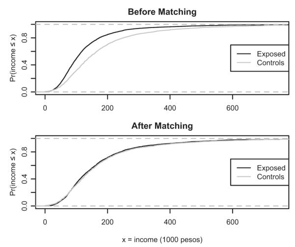
Cumulative distribution of household total per capita income for exposed and control groups before and after matching. The cumulative distribution is the proportion of persons with income less than or equal to x. Before matching, exposed subjects had lower income. After matching for KS distance, the entire distributions are almost the same. The KS distance is the largest vertical distance between the two curves.

Effect on PTSS

Table 3 illustrates heterogeneous effects for the one question about difficulty falling asleep,³³ although ignoring who is paired with whom. Many more persons who were exposed to the earthquake when compared with controls reported extensive difficulty in sleeping, and yet more than half of the exposed respondents (1,382/2,520 = 55%) reported no difficulty. Similar patterns were present for the other symptoms.

Figure 3 looks at all 17 symptoms, depicting the exposed-minus-control pair difference in Davidson Trauma Scores. Figure 3 has a density estimate or smoothed histogram (from density in R). If the effect of the earthquake were constant—the same for every exposed person—then the density would be symmetric about that constant value, and the constant could be estimated as the coefficient of an indicator or dummy variable in a regression. However, that is not what we see in Figure 3. The density is sharply skewed right, with large positive differences occurring much more often than large negative differences—and yet the mode or peak is close to zero. Many pairs exhibit no indication of PTSS, whereas some pairs exhibit large positive differences in PTSS; thus it would be a mistake to estimate the effect of the earthquake on PTSS as the coefficient of an indicator, or as a mean, median, or other typical difference. For instance, the point estimate for the typical difference based on inverting the Wilcoxon’s test is 20.0 (95% CI = 18.5–21.0); however, these and similar measures assume a constant effect, and so they are very misleading. It appears that some people are severely affected and others less affected: a typical effect of 20 misrepresents many negligible effects and some dramatic effects. If the effects were a constant effect of 20, then Figure 3 would be symmetric about 20, which it clearly is not.

FIGURE 3.

Exposed-minus-control matched-pair differences in posttraumatic stress symptoms (PTSS) scores for 2520 matched pairs. The upper figure is a nonparametric density estimate (using default settings in R) and the lower figure is a box plot. To aid the eye, the vertical line is at zero difference. The graphs indicate that many pair differences were close to zero, consistent with no difference in symptoms, but differences that were far from zero were mostly positive: when PTSS differed, it was the exposed person who typically experienced severe symptoms.

Recall from the Methods section that Stephenson’s³¹ statistic looks at all subsets of m = 8 pairs and estimates the probability that the largest absolute difference in m = 8 pairs has higher PTSS for the exposed person than the control. A probability of ½ suggests no effect of the earthquake. In Figure 3, the estimate of the probability for m = 8 is not 0.5, but rather 0.96 (with one-sided 95% CI from ref. 21 of 0.91–1.00); that is, in 8 pairs, the largest absolute difference is a positive difference 96% of the time, with a larger trauma score for the exposed person than the control. In a matched pair, if there is a substantial difference in PTSS, it is almost always the exposed subject who has greater symptoms.

Moving away from the naive assumption that adjustments for observed covariates remove all bias, we examine the sensitivity of this finding to biases of specific magnitudes.^{14,15(§4),21} Bias is measured by a parameter Γ that describes a pair of one exposed and one control subject matched on the 46 observed covariates: it says their relative risk of exposure to the earthquake may be as high as Γ or as low as 1/Γ owing to differences in unobserved covariates.^{19,expression 1} In a clinical trial, random assignment of treatments ensures Γ = 1; that is, each subject in a pair has the same ½ chance of receiving the treatment, with relative risk of treatment of (½)/(½) = 1. If Γ = 2, one subject might have a probability as high as 2/3 of treatment, the other as low as 1–2/3 = 1/3, so the relative risk of exposure to the treatment is at most (2/3)/(1/3) = 2. Thus, Γ = 2 is a moderately large departure from a randomized experiment. We ask how much bias, measured by Γ, would be needed for the naive 95% CI (0.91–1.00) in the previous paragraph to be moved to include 0.5 and smaller effects, which would imply that even the sign of the effect is in doubt. For this, 95% interval to include 0.5 owing to biased exposure to the earthquake, an exposed and a control subject matched on the 46 observed covariates would need to differ in their relative risk of exposure to the earthquake by a factor of more than Γ = 14 attributable to an unobserved covariate not controlled by the matching. This covariate would need to be a near-perfect predictor of posttraumatic stress. (More precisely, the two-sided 95% CI just covers 0.5 for Γ = 14.6.) If the unobserved covariate were less than a perfect predictor of posttraumatic stress, then it would need to increase the relative risk of exposure by a factor of more than 30, and increase the relative risk of a positive difference in PTSS by a factor of more than 30 to explain the observed association (ie, Γ = 14 amplifies to Λ = 30 and Δ = 30 in the notation Rosenbaum and Siber³⁴). For comparison, Hammond’s³⁵ study of heavy smoking as a cause of lung cancer (one of the least sensitive studies in epidemiology^{15(Table 4.1)} becomes sensitive at Γ = 6.

If Wilcoxon’s statistic (m = 2) is used, the difference in PTSS is judged more sensitive to unmeasured bias, becoming sensitive at Γ = 6.0, rather than Γ = 14 for m = 8. For m = 20, also evaluated in ref. 19, the difference in PTSS becomes sensitive at Γ = 22.4. If one looks at the largest absolute difference in PTSS in all sets of m = 20 pairs, the difference is positive 98% of the time reflecting greater symptoms for the exposed individual in the pair, as distinct from 96% of the time for m = 8 as seen earlier. This pattern is expected for a treatment that harms some people and spares many others.

The eAppendix (http://links.lww.com/EDE/A637) presents parallel analyses for (1) subgroups defined by sex, age, and ethnic group; (2) pairs reporting no physical health problems; (3) standard subscores of the Davidson Trauma Scale; and (4) a subscore that avoids reference to specific trauma. These analyses vary slightly, with somewhat greater PTSS for women, and for older people, but the difference in PTSS has the same form as Figure 3 in all subgroups and subscores, and it is highly insensitive to unmeasured biases.

DISCUSSION

The Chilean earthquake offered a unique opportunity to assess the effect of trauma on PTSS because of longitudinal data free of recall bias, with detailed information about the same people before and after the earthquake. Guided by the statistical theory of design sensitivity,^16–18 the comparison was designed to be as insensitive as possible to biases from unmeasured covariates; in the end, the results were indeed highly insensitive. Specifically, severely shaken regions of Chile were compared with untouched regions, and exposure to the earthquake had a strong and heterogeneous effect on PTSS. In particular, in 96% of pairs exhibiting substantial PTSS, the exposed rather than the unexposed person exhibited elevated symptoms (95% CI = 91–100%). Because heterogeneous effects were anticipated, statistical techniques with power to detect such effects were used.

Combining standard^17,22 and new^23,30 techniques, the matching balanced 46 observed covariates measured before the earthquake, including socioeconomic status, housing quality, health, and health insurance.

Figure 3 shows the heterogeneous pattern of PTSS effects in pairs that are similar in 46 covariates. Adjustment for covariates using a model would not yield a simple depiction of heterogeneous effects among similar people. Indeed, some model-based analyses never entertain the possibility of heterogeneous treatment effects, instead estimating a typical effect as the coefficient of an exposure indicator in a model. If only a subset of exposed persons responds to exposure, an estimate of a typical effect may miss a stable and substantial atypical effect.^20,21

Advice about study design from design sensitivity derives from mathematical proof and simulation^11–13; however, the advice is intuitively sensible. Ever since the first sensitivity analysis,¹⁰ it has been known that larger treatment effects are less sensitive than smaller effects; however, the meaning of this, once one moves beyond the 2 × 2 table, is unclear. If a treatment strongly affects some people and leaves others unaffected, then is that a large effect? The mean or median effect may be small, but the effect on affected persons may be large and unambiguous (Fig. 3). Statistics built to detect heterogeneous effects^20,21 judge this to be a large effect, hence an effect insensitive to small unmeasured biases.^{17(§16),18(§6.6)} When two (or more) patterns of effect are plausible, an appropriate analysis may look for two patterns correcting for multiplicity.³⁶ Similarly, if more intense treatment produces larger effects, the largest and therefore least sensitive effects will be found in a comparison of intense exposure and no exposure.16,17(§17.3),18(§6.4) We have discussed design sensitivity as it is relevant to the study of the earthquake in Chile; other aspects of design sensitivity are not discussed here but may be relevant to other studies.^17,18

Matching was done using the new R package mipmatch.²³ Once installed mipmatch is fairly straightforward to use, but installation is not as simple as for most R packages because IBM’s CPLEX must also be installed. IBM makes CPLEX available for free to academics. The mipmatch package does some unique things, such as finely balancing many variables at once, force balancing on the mean of a continuous variable, and balancing a continuous variable such as income at every quantile. However, somewhat less general packages, such as Hansen’s optmatch³⁷ and Yang’s fine balance,²⁹ produce excellent matched comparisons, and install effortlessly. Hansen’s optmatch is illustrated in Rosenbaum.^17(§13) Software in R and a practice session for the sensitivity analysis are in the online appendix to ref. 19.

One limitation is that our PTSS information is based on self-report. There is no evidence internal to the survey about the relation between self-reported symptoms and what a psychiatrist would determine. It is conceivable that a natural disaster reduces stigma associated with reporting PTSS and this might account for some of the increase in reported symptoms.

PTSS were dramatically but unevenly elevated among residents of strongly shaken areas of Chile when compared with similar people in largely untouched parts of the country. Contrary to some prior expectations,³⁸ exposure to disasters is less equitable than random. Residents of highly affected areas had less education, lower income, and lower employment, and they lived in cheaper housing; however, these measured differences could be removed by matching. The exposure may have been inequitable in other unmeasured ways, as well, but the sensitivity analysis shows that these unmeasured biases would need to be very large to negate the main conclusions.

REFERENCES

- 1. [Accessed 8 June 2012];United States Geological Survey. Available at: http://earthquake.usgs.gov/earthquakes/world/10_largest_world.php; http://earthquake.usgs.gov/earthquakes/recenteqsww/Quakes/us2010tfan.php#summary.
- 2.Neria Y, Nandi A, Galea S. Post-traumatic stress disorder following disasters: a systematic review. Psychol Med. 2008;38:467–480. doi: 10.1017/S0033291707001353. [DOI] [PMC free article] [PubMed] [Google Scholar]
- 3.Goenjian AK, Steinberg AM, Najarian LM, Fairbanks LA, Tashjian M, Pynoos RS. Prospective study of posttraumatic stress, anxiety, and depressive reactions after earthquake and political violence. Am J Psychiatry. 2000;157:911–916. doi: 10.1176/appi.ajp.157.6.911. [DOI] [PubMed] [Google Scholar]
- 4.Rutter M. Resilience in the face of adversity. Protective factors and resistance to psychiatric disorder. Br J Psychiatry. 1985;147:598–611. doi: 10.1192/bjp.147.6.598. [DOI] [PubMed] [Google Scholar]
- 5.Bonanno GA. Loss, trauma, and human resilience: have we underestimated the human capacity to thrive after extremely aversive events? Am Psychol. 2004;59:20–28. doi: 10.1037/0003-066X.59.1.20. [DOI] [PubMed] [Google Scholar]
- 6.McLaughlin KA, Fairbank JA, Gruber MJ, et al. Serious emotional disturbance among youths exposed to Hurricane Katrina 2 years postdisaster. J Am Acad Child Adolesc Psychiatry. 2009;48:1069–1078. doi: 10.1097/CHI.0b013e3181b76697. [DOI] [PMC free article] [PubMed] [Google Scholar]
- 7.Galea S, Tracy M, Norris F, Coffey SF. Financial and social circumstances and the incidence and course of PTSD in Mississippi during the first two years after Hurricane Katrina. J Trauma Stress. 2008;21:357–368. doi: 10.1002/jts.20355. [DOI] [PubMed] [Google Scholar]
- 8.Roemer L, Litz BT, Orsillo SM, Ehlich PJ, Friedman MJ. Increases in retrospective accounts of war-zone exposure over time: the role of PTSD symptom severity. J Trauma Stress. 1998;11:597–605. doi: 10.1023/A:1024469116047. [DOI] [PubMed] [Google Scholar]
- 9.David AC, Akerib V, Gaston L, Brunet A. Consistency of retrospective reports of peritraumatic responses and their relation to PTSD diagnostic status. J Trauma Stress. 2010;23:599–605. doi: 10.1002/jts.20566. [DOI] [PubMed] [Google Scholar]
- 10.Cornfield J, Haenszel W, Hammond EC, et al. Smoking and lung cancer: recent evidence and a discussion of some questions. J Natl Cancer Inst. 1959;22:173–203. [PubMed] [Google Scholar]
- 11.Marcus SM. Using omitted variable bias to assess uncertainty in the estimation of an AIDS education treatment effect. J Educ Stats. 1997;22:193–201. [Google Scholar]
- 12.Rosenbaum PR, Rubin DB. Assessing sensitivity to an unobserved binary covariate in an observational study with binary outcome. J Roy Stat Soc B Met. 1983;45:212–218. [Google Scholar]
- 13.Yanagawa T. Case-control studies: assessing the effect of a confounding factor. Biometrika. 1984;71:191–194. [Google Scholar]
- 14.Rosenbaum PR. Sensitivity analysis for certain permutation tests in matched observational studies. Biometrika. 1987;74:13–26. [Google Scholar]
- 15.Rosenbaum PR. Observational Studies. 2nd ed Springer; New York, NY: 2002. [Google Scholar]
- 16.Rosenbaum PR. Design sensitivity in observational studies. Biometrika. 2004;91:153–164. [Google Scholar]
- 17.Rosenbaum PR. Design of Observational Studies. Springer; New York, NY: 2010. [Google Scholar]
- 18.Rosenbaum PR. What aspects of the design of an observational study affect its sensitivity to bias from covariates that were not observed? In: Dorans N, Sinharay S, editors. Looking Back: Proceedings of a Conference in Honor of Paul W. Holland. Springer; New York, NY: 2011. pp. 87–114. [Google Scholar]
- 19.Rosenbaum PR. [Accessed 19 November 2012];A new u-statistic with superior design sensitivity in observational studies. Biometrics. 2011 67:1017–1027. doi: 10.1111/j.1541-0420.2010.01535.x. R-software/instructions. Available at: http://www-stat.wharton.upenn.edu/~rosenbap/rsession.txt. [DOI] [PubMed] [Google Scholar]
- 20.Conover WJ, Salsburg DS. Locally most powerful tests for detecting treatment effects when only a subset of patients can be expected to “respond” to treatment. Biometrics. 1988;44:189–196. [PubMed] [Google Scholar]
- 21.Rosenbaum PR. Confidence intervals for uncommon but dramatic responses to treatment. Biometrics. 2007;63:1164–1171. doi: 10.1111/j.1541-0420.2007.00783.x. [DOI] [PubMed] [Google Scholar]
- 22.Stuart EA. Matching methods for causal inference: a review and a look forward. Stat Sci. 2010;25:1–21. doi: 10.1214/09-STS313. [DOI] [PMC free article] [PubMed] [Google Scholar]
- 23.Zubizarreta JR. Using mixed integer programming for matching in an observational study of kidney failure after surgery. J Am Statist Assoc. 2012 accepted. R software mipmatch at http://www-stat.wharton.upenn.edu/~josezubi/ [Google Scholar]
- 24.Peto R, Pike MC, Armitage P, et al. Design and analysis of randomized clinical trials requiring prolonged observation of each patient. I. Introduction and design. Br J Cancer. 1976;34:585–612. doi: 10.1038/bjc.1976.220. [DOI] [PMC free article] [PubMed] [Google Scholar]
- 25.Davidson JR, Book SW, Colket JT, et al. Assessment of a new self-rating scale for post-traumatic stress disorder. Psychol Med. 1997;27:153–160. doi: 10.1017/s0033291796004229. [DOI] [PubMed] [Google Scholar]
- 26.Rosenbaum PR, Rubin DB. The central role of the propensity score in observational studies for causal effects. Biometrika. 1983;70:41–55. [Google Scholar]
- 27.Rosenbaum PR. Optimal matching in observational studies. J Am Statist Assoc. 1989;84:1024–1032. [Google Scholar]
- 28.Rosenbaum PR, Ross RN, Silber JH. Minimum distance matched sampling with fine balance in an observational study of treatment for ovarian cancer. J Am Statist Assoc. 2007;102:75–83. [Google Scholar]
- 29.Yang D, Small DS, Silber JH, Rosenbaum PR. Optimal matching with minimal deviation from fine balance in a study of obesity and surgical outcomes. Biometrics. 2012;68:628–636. doi: 10.1111/j.1541-0420.2011.01691.x. [DOI] [PMC free article] [PubMed] [Google Scholar]
- 30.Zubizarreta JR, Reinke C, Kelz RR, et al. Matching for several sparse nominal variables in a case-control study of readmission following surgery. Am Stat. 2011;65:229–238. doi: 10.1198/tas.2011.11072. [DOI] [PMC free article] [PubMed] [Google Scholar]
- 31.Stephenson WR. A general class of one-sample nonparametric test statistics based on subsamples. J Am Stat Assoc. 1981;76:960–966. [Google Scholar]
- 32.Salsburg D. Alternative hypotheses for the effects of drugs in small-scale clinical studies. Biometrics. 1986;42:671–674. [PubMed] [Google Scholar]
- 33.Lavie P. Sleep disturbances in the wake of traumatic events. N Engl J Med. 2001;345:1825–1832. doi: 10.1056/NEJMra012893. [DOI] [PubMed] [Google Scholar]
- 34.Rosenbaum PR, Silber JH. Amplification of sensitivity analysis in matched observational studies. J Am Stat Assoc. 2009;104:1398–1405. doi: 10.1198/jasa.2009.tm08470. [DOI] [PMC free article] [PubMed] [Google Scholar]
- 35.Hammond EC. Smoking in relation to mortality and morbidity. findings in first thirty-four months of follow-up in a prospective study started in 1959. J Natl Cancer Inst. 1964;32:1161–1188. [PubMed] [Google Scholar]
- 36.Rosenbaum PR. Testing one hypothesis twice in observational studies [published online ahead of print 24 July 2012] Biometrika. doi: 10.1093/biomet/ass032. [Google Scholar]
- 37.Hansen BB. Optmatch. R News. 2007;7:18–24. [Google Scholar]
- 38.Bromet EJ, Havenaar JM. Mental health consequences of disasters. In: Sartorius N, Gaebel W, López-Ibor J, et al., editors. Psychiatry in Society. John Wiley & Sons; Chichester, UK: 2002. [Google Scholar]
Associated Data
This section collects any data citations, data availability statements, or supplementary materials included in this article.