Quantum Dynamics in Continuum for Proton Transport I: Basic Formulation

Abstract

Proton transport is one of the most important and interesting phenomena in living cells. The present work proposes a multiscale/multiphysics model for the understanding of the molecular mechanism of proton transport in transmembrane proteins. We describe proton dynamics quantum mechanically via a density functional approach while implicitly model other solvent ions as a dielectric continuum to reduce the number of degrees of freedom. The densities of all other ions in the solvent are assumed to obey the Boltzmann distribution. The impact of protein molecular structure and its charge polarization on the proton transport is considered explicitly at the atomic level. We formulate a total free energy functional to put proton kinetic and potential energies as well as electrostatic energy of all ions on an equal footing. The variational principle is employed to derive nonlinear governing equations for the proton transport system. Generalized Poisson-Boltzmann equation and Kohn-Sham equation are obtained from the variational framework. Theoretical formulations for the proton density and proton conductance are constructed based on fundamental principles. The molecular surface of the channel protein is utilized to split the discrete protein domain and the continuum solvent domain, and facilitate the multiscale discrete/continuum/quantum descriptions. A number of mathematical algorithms, including the Dirichlet to Neumann mapping, matched interface and boundary method, Gummel iteration, and Krylov space techniques are utilized to implement the proposed model in a computationally efficient manner. The Gramicidin A (GA) channel is used to demonstrate the performance of the proposed proton transport model and validate the efficiency of proposed mathematical algorithms. The electrostatic characteristics of the GA channel is analyzed with a wide range of model parameters. The proton conductances are studied over a number of applied voltages and reference concentrations. A comparison with experimental data verifies the present model predictions and validates the proposed model.

1 Introduction

Proton transport is of central importance and plays a major role in many biochemical processes, such as cellular respiration, ATP synthase, photosynthesis and denitrification [28]. Energy transduction in a bioenergetic system requires the generation of large proton concentration gradients. For example, the chemical energy is stored as proton gradient that drives the ATP generation in mitochondria. For plants, light energy is transduced into a proton gradient to create ATP in chloroplasts [20]. Another important function of voltage-gated proton channels occur in phagocytes, such as human neutrophils, during the respiratory burst process. The proton efflux through the proton channels balances the electron movement generated by the NADPH oxidase and assists the production of extracellular reactive oxygen species that kill bacteria. However, main mechanism of proton transport is not fully understood yet [42], with the belief that the proton has distinguished properties from those of other cations and has significantly different conductivity. The motion of regular ions in solvent is usually described as diffusion, while the proton is interchangeable with protons that form water molecules, then it may translocate through a succession of hops in the hydrogen-bond network as indicated by the Grotthuss theory [33]. The proton has the lightest mass among all ions and an effective radius that is at least 10⁵ smaller than other ions because the H⁺ has no electron [20]. The light mass and tiny size greatly facilitate proton transfer reaction and electrostatic interactions with surrounding molecules [32]. Due to these unique physical properties, the mobility of protons in bulk solution is about fivefold higher than that of other cations [2]. The proton permeation across the membrane is also quite different. Regular ions are prohibited to permeate the membrane because of the huge energy barrier formed by the bilayer. They can only transport through the membrane with the assistance of ion channels, which form water pores and guide ions by diffusion and electrostatic potentials.

Transport pathways of proton across the membrane can have various mechanisms. Protons can achieve the translocation by means of hydrogen-bonded chain (HBC) [22], which may consist not only water molecules, but also side groups of amino acids capable of forming hydrogen bonds. In this sense, proton can transport through the membrane when the row of water molecules is not continuous, since the HBC can be connected by the one from side chains of amino acids of membrane proteins. Moreover, proton may permeate phospholipid membrane even when membrane proteins are absent. For example, a chain of water molecules could happen to line up across the membrane due to thermal fluctuations [23] and provide the HBC to conduct protons. Naturally, protons can transport in water-filled channel pores as well, such as the Gramicidin A (GA) and other “normal” cation-selective channels. However, transport motion of protons in the narrow channel pore is quite different from that in the bulk solvent. Since the length and angle of hydrogen bonds are critically important, the geometry of the membrane channel pore plays an essential role. It has been pointed out that the proton transport in a narrow water-filled pore might behave more like proton conduction in ice than in liquid water because water molecules inside heavily confined spaces are greatly restricted in the sense of diffusion and reorientation, i.e., the water inside narrow channels is to some extent “frozen” [6, 38]. Meanwhile, some physical properties, such as the polarizability of water and diffusivity of proton decrease with the diameter of the confined space [4]. There is general consensus that any restriction of water mobility in the channel pore will tend to reduce proton mobility. One more mechanism for proton transport is voltage-gated proton channels, which are extremely H⁺ selective, large temperature dependent channel proteins. Voltage-gated proton channels are usually not water-filled pores so the HBC contains at least one amino acid side group.

There are several strategies in modeling a general ion transport process. Molecular dynamics (MD) provides one of the most detailed descriptions in modeling biomolecular systems and there are several user-friendly packages available, such as AMBER [34], CHARMM [30], etc. However, a significant hurdle in the MD prediction of the channel conductance is the necessarily small time step (10⁻¹⁵ second) versus the ion permeation time scale (10⁻⁶ second) [15]. Brownian dynamics (BD) [14] and the Poisson-Nernst-Planck (PNP) theory [9,16,46] are utilized to study ion channels based on the mean-field approximation. In the former approach, ions are treated as explicit particles in the ion channel, interacting with surrounding environments (channel proteins and lipid bilayers). In the PNP model, not only the protein, lipid layer, bath solution, but also the ions of interest are all modeled as continuums through electro-diffusion theory. Both the BD and PNP models have a number of similarities in their initial setups and computational approaches [24, 31]. There is an agreement that the BD theory and PNP model may be expected to work well for regular ions but not for protons [15], which have lighter mass and whose transport involves the hydrogen bonds making and breaking as mentioned above. The proton transport process is special and needs to be studied quantum mechanically. Some investigators have explored proton channels via Feynman path integral simulations and quantum energy levels of protons are computed by the Schrödinger equation [35]. Several theoretical models are proposed in the last decade [5, 40,42].

The objective of the present work is to propose a multiscale quantum dynamics in continuum (QDC) model for the prediction and analysis of the proton translocation across transmembrane channels. The structure of the membrane protein is taken into account during the proton transport, with which the model has the potential ability to study more complicated voltage-gated proton channel in the future. The proton transport mechanism along the water chain, cooperated with the structure of the membrane protein is studied in this work. To this end, a simple but typical ion channel, the Gramicidin A (GA) is utilized as the membrane protein, in which the proton transport along the water molecules is studied. We describe the dynamics of protons quantum mechanically while represent the density of other ions by the Boltzmann distribution, which is in a quasi-equilibrium due to the change of the electrostatic potential during the proton transmembrane permeating process [47]. Since van der Waals interactions involve less energy compared to electrostatic ones, numerous solvent molecules are implicitly treated as a dielectric continuum to reduce the number of degrees of freedom of the system. The impact of protein molecular structure and its fixed charges to the proton transport is explicitly considered in our model. We propose a total free energy framework to put the kinetic and potential energies of protons and the electrostatic energy of the whole system, i.e., all ions, channels protein and lipid bilayer, on an equal footing. By using the variational principle, we derive governing equations of the Poisson-Boltzmann and Kohn-Sham types for the proton transport system. There are a few reasons for us to employ the present quantum mechanical description. First, the proton transport mechanism is different and the hydro-dynamic approximation is not valid any more. Secondly, conceptually the ion concentration is no longer well defined in a small-size channel. Instead, the probability density function is used for protons. Moreover, many water-filled channels are very narrow with extremely small local diameters around 2Å [39], which implies a strong confinement in the transverse direction.

The rest of the present paper is organized as follows. Section 2 is devoted to the theory and model. We present a variational paradigm for analyzing proton transport. Our model incorporates quantum mechanical treatment of protons, classical description of electrostatics, and atomic detail of protein structure and charges. Formalisms for proton density and transport are derived from fundamental principles. Section 3 discusses numerical implementation and computational algorithms. The molecular surface [37] is employed to separate the discrete/continuum domains and facilitate the quantum/classical descriptions. To simplify the computation, we adopt a decomposition approximation to split the proton transport direction from the transverse confined directions. Mathematical ingredients of this quantum/discrete/continuum model include coupled nonlinear partial differential equations (PDEs) and the elliptic PDEs with discontinuous coefficients and singular sources. Therefore, the corresponding numerical algorithms, the matched interface and boundary (MIB) method, the Dirichlet-to-Neumann mapping (DNM) and Krylov space iteration schemes are equipped to implement the numerical simulations. In Section 4, we employ a commonly used channel protein, the Gramicidin A (GA), to demonstrate the performance of the proposed theoretical model and validate the proposed computational algorithms. Electrostatic properties are analyzed with a number of combinations of model parameters to gain a basic understanding of the GA channel. The conductance of protons under various external voltages and concentrations are simulated. Comparison is made with experimental measurements in the literature. This paper ends with a brief conclusion.

2 Theory and model

In this section we provide the theoretical formulation of our model of quantum dynamics in continuum.

2.1 General description of the model

we propose a multiscale, multiphysics and multidomain model for the proton transport through membrane channels. The computational domain Ω is divided into two subdo-mains, i.e., the solvent subdomain Ω_s consisting of the extracellular/intracellular solvent regions plus channel pore region, and the biomolecular subdomain Ω_m including the membrane protein(s) as well as lipid bilayers. Therefore, we have Ω = Ω_s∪Ω_m. A detailed graph of these subdomains is given in Fig. 1. The interface Γ between solvent-membrane protein is defined by the molecular surface generated by the MSMS software package [37]. It is interesting to note. that the physics in each subdomain is very different and there are multiphysics phenomena even in a single subdomain. For the biomolecular subdomain, the membrane protein and lipid bilayer structural data are either generated by molecular dynamics simulations, or downloaded from the Protein Data Bank (PDB) which contains data collected from X-ray crystallography or nuclear magnetic resonance (NMR) experiments. The force field parameters, such as atomic van der Waals radii and point charges, are obtained from the CHARMM force field [30].

Figure 1.

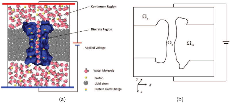
(a) Illustration of multiscale model of proton transport through a water-filled channel; (b) Illustration of an x–z cross section of computational domains of the multiscale model with Ω_m being the channel molecule and membrane subdomain and Ω_s being the solvent subdomain. Here z-direction is regarded as the transport direction.

In the solvent subdomain, there are three types of materials: protons, all other ion species and water molecules. To reduce the number of degrees of freedom, we treat solvent (water) molecules as dielectric continuum background or bath. In the bath region, all ions are essentially in a quasi-equilibrium state and their densities are well described by the Boltzmann distribution except for at the solvent-membrane protein interface. Near the solvent-membrane protein interface, the density distribution of ions might be better described by the density functional theory of solution, or integral equations, in which the dispersion interaction between solvent and solute can be better accounted. This effect is modeled as generalized-correlation potential effect in the present work.

The physics in the channel pore region is of central interest and is sharply different from those of other regions. There are many evidences which indicate the quantum mechanical behavior of proton transfer in biomolecular systems and proton channels [3,17]. The first reason is the small mass of a proton which enhances the quantum tunneling effect in the proton transport. Additionally, a narrow water-filled channel morphology might lead to severe quantum confinement, which consequently promotes quantum effects. Finally, the hydrogen-bonded chain of water molecules assisted proton translocation is quantum mechanical in origin [35]. For these reasons, we treat protons quantum mechanically via a scattering formalism which describes how a quantum mechanical proton scatters through electrostatic and generalized-correlation potential fields. The electrostatic potentials include interactions between protons represented by a self-consistent mean field approximation, the interactions between protons and fixed ions from membrane proteins and lipid bilayers, and the interactions between protons and other ion species. The generalized-correlation potential is due to the impacts of the continuum solvent, the van der Waals interaction between the solvent and biomolecules, the effect of ion-water clusters, dispersion effect, and possible break-down of hydrogen-bonded chain in a narrow channel, etc. We utilize a total energy functional framework [10,11,43] to incorporate quantum mechanical description and continuum description. Coupled Kohn-Sham equation for the proton dynamics and Poisson-Boltzmann equation for the electrostatic potential are derived from the variational principle. Solutions to these coupled equations give rise to proton structural dynamics, and transport process, which describes how a quantum mechanical proton scatters through electrostatic and generalized-correlation potential fields.

2.2 Free energy components

This subsection describes various free energy components in our multiscale model of quantum dynamics in continuum. In order to give a clear description, Fig. 1(a) is reduced to a sketch in Fig. 1(b) in x − z cross section, where the z direction represents the proton transport direction: the system is restricted to a rectangular cuboid with appropriate size and partitioned into two different computational domains. The permittivity ∊(r) has different values in two domains

$$∊\left(\mathrm{r}\right)=\{\begin{array}{cc}{∊}_s\left(\mathbf{r}\right)& \forall \mathbf{r}\in {\Omega }_s\\ {∊}_m\left(\mathbf{r}\right)& \forall \mathbf{r}\in {\Omega }_m\end{array}.$$ (2.1)

With ∊_s(r) = 0 if r ∈ Ω_m and ∊_m(r) = 0 if r ∈ Ω_s. Since both the membrane and channel protein are treated with same dielectric medium, the interface between them is erased and a constant dielectric constant is assumed on Ω_m. The solvent in the bath regions and in the channel pore have different biological characteristics. Therefore the position dependent dielectric constant is imposed on the solvent subdomain Ω_s. In fact, ∊_s(r) in the channel region can differ much from that in the bulk region. The detailed discussion about the dielectric constants is given in Section 3.5. There are three major categories of macroscopic variables in the model which are defined in different subdomains and formulated in classical and quantum mechanisms.

2.2.1 Electrostatic free energy in the biomolecular region

The biomolecular region consists of membrane protein and lipid bilayer. Their structures essentially determine the interactions between protons and protein, so it is necessary to account the structures in atomic details. In the present treatment, we assume that structures of membrane protein and lipid bilayer are given and do not change during the ion transport process. This is certainly an approximation and will be easily removed in our future work by a combination of the present formulation with MD simulations [43]. Without structural cooperation, the biomolecules still significantly contribute to ion dynamics and transport by electrostatic interactions. The fixed charges in the channel protein and nearby lipid bilayers determine the fundamental characteristics of the channel and provide the primary environment for ions' permeation. Since the total number of fixed charges is not too large (i.e., up to thousands), with the assumption that the positions of them are essentially fixed, the explicit discrete description is actually affordable. In this sense, they serve as a source term in the electrostatic potential calculation

$${\rho }_f\left(\mathbf{r}\right)=\sum _{i=1}^{N_a}{Q}_i\delta \left(\mathbf{r}-{\mathbf{r}}_i\right)$$ (2.2)

where N_a is the total number of fixed charges, Q_i and r_i are the point charge and position of the ith atom. Therefore, the electrostatic free energy in biomolecular domain is given by [43]

$$G_{\text{Mol}}\left[\Phi ,n\right]=\int \left[\frac{{∊}_m\left(\mathbf{r}\right)}{2}{\left|\nabla \Phi \right|}^2-\Phi {\rho }_f\right]d\mathbf{r},$$ (2.3)

where Φ(r) is the electrostatic potential and is defined on the whole domain Ω_s∪Ω_m.

2.2.2 Electrostatic free energy in the solvent region

Ions in the solvent region also contribute to the electrostatic potential. Protons and other ion species are treated in different manners. Let us denote the proton number density in the solvent region as n(r) and the charge density as ρ_p = qn(r), q is the elementary charge or charge carried by a single proton. The charge density serves as a source term in the electrostatic free energy.

In the solvent region, particularly, in the extracellular and intracellular solvent regions, apart from ions of interest, there are many other ions. In the present model, all other ions are treated in a different manner from the ions of interest. Specifically, no detailed description is given to individual ions except for the ions of interest. However, other ions contribute considerably to the electrostatic property of the whole system. To account for their electrostatic effort, we describe other ions by using the Boltzmann distribution [47]. The charge density of other ions is given by

$${\rho }^{\prime }=\sum _j^{N_c^{\prime }}{q}_j{n}_j^{\prime }\left(\mathbf{r}\right)=\sum _j^{N_c^{\prime }}{q}_j{n}_j^0{e}^{-\frac{q_j\Phi \left(\mathbf{r}\right)-{\mu }_j}{k_{B}T}},$$ (2.4)

where $N_c^{\prime }$ is the total number of other ion species, $n_j^0$ and q_j are the bulk constant density and charge of the jth ion species. Here $n_j^{\prime }=n_j^0{e}^{-\left(q_j\Phi \left(\mathbf{r}\right)-{\mu }_j\right)/k_{B}T}$ is the number density of jth ion species. It can be noticed that the Boltzmann distribution of the other ion species with respect to the potential has been modified with μ_j, the relative chemical potential of the jth ion species [36,46].

The corresponding electrostatic free energy in the solvent region is given by

$$G_{\text{Sol}}[\Phi ]=\int \left[\frac{{∊}_s\left(\mathbf{r}\right)}{2}{\left|\nabla \Phi \left(\mathbf{r}\right)\right|}^2-\Phi \left(\mathbf{r}\right){\rho }_p\left(\mathbf{r}\right)+k_{B}T\sum _j^{N_c^{\prime }}{n}_j^0\left(e^{-\frac{q_j\Phi \left(\mathbf{r}\right)-{\mu }_j}{k_{B}T}}-1\right)\right]d\mathbf{r},$$ (2.5)

Note that the electrostatic free energy of other ions in Eq. (2.5) is similar in spirit to Sharp and Honig [41], Gilson et al [27], Chen et al [11] and Wei [43].

2.2.3 Proton free energies and interactions

The solvent region might admit a number of ion species, of which a full quantum model can be technically complicated and computationally time consuming. We therefore only treat the ions of interest, i.e., protons, quantum mechanically and assume a continuum description of other ion species. To simplify the problem further, we consider a generalized density functional theory for protons.

Kinetic energy

The proton density operator n_H is given by [10]

$$n_H=e^{-\frac{H-{\mu }_p}{k_{B}T}}$$ (2.6)

where H is the Hamiltonian of the system and μ_p is the relative chemical potential of protons. We define the proton density n(r) as

$$n\left(r\right)=\langle r\left|n_H\right|r\rangle =\int {\left|{\Psi }_E\left(r\right)\right|}^2{e}^{-\frac{E-{\mu }_p}{k_{B}T}}dE,$$ (2.7)

where Ψ_E and E are the wavefunction and corresponding energy associated with H. The Boltzmann statistics is adopted in the present work. The number density gives rise to the total number of protons in the system, i.e.,

$${\int }_{{\Omega }_s}n\left(\mathbf{r}\right)d\mathbf{r}=N_p.$$ (2.8)

However, in most experimental set-ups, one does not know N_p. Instead, the bulk concentration or the bulk number density, $n_p^0$, is given. When the solvent domain is sufficiently large compared to the channel pore region, one has two approximations

$$N_p\cong n_p^0{\int }_{{\Omega }_s}{e}^{-\frac{q\Phi \left(r\right)-\mu p}{k_B^T}}dr\cong n_p^0{\int }_{{\Omega }_s}d\mathbf{r},$$ (2.9)

where the second approximation is a crude estimation.

The kinetic energy is given by $\frac{{\mathbf{p}}^2}{2\mathit{m}\left(\mathbf{r}\right)}$ where p is the momentum and m is proton effective mass. In the coordinate representation, the kinetic energy of protons can be given as

$$\iint \frac{{\hslash }^2{e}^{-\left(E-{\mu }_p\right)/k_{B}T}}{2m\left(r\right)}{\left|\nabla {\Psi }_E\left(r\right)\right|}^2\mathit{dEd}\mathbf{r},$$ (2.10)

where the Boltzmann factor weights different energy contributions.

Electrostatic potential

Protons have a number of electrostatic interactions. First, protons interact repulsively among themselves

$$U_{\text{Ion}-\text{Ion}}\left(\mathbf{r}\right)=\frac{1}{2}\int \frac{q^{2}n\left(\mathbf{r}\right)n\left({\mathbf{r}}^{\prime }\right)}{∊\left(\mathbf{r}\right)\left|\mathbf{r}-{\mathbf{r}}^{\prime }\right|}d{\mathbf{r}}^{\prime }.$$ (2.11)

These interactions lead to a term that is nonlinear in density n and the resulting equations are to be solved iteratively.

Additionally, interactions between protons in the solvent and fixed charges in biomolecules are described as

$$U_{\text{Ion}-\text{Fix}}\left(\mathbf{r}\right)=\sum _{i=1}^{N_a}\frac{\mathit{q}\left(\mathbf{r}\right)Q_i}{∊\left(\mathbf{r}\right)\left|\mathbf{r}-{\mathbf{r}}_i\right|}.$$ (2.12)

This contribution can be handled by the so called Dirichlet to Neumann mapping approach [10].

Finally, interactions between protons and other ion species are of the form

$$U_{\text{Ion}-\text{Other}}\left(\mathrm{r}\right)\sum _{j1}^{{N^{\prime }}_c}\int \frac{q{q}_{j}n\left(\mathbf{r}\right){n^{\prime }}_j\left({\mathbf{r}}^{\prime }\right)}{\varepsilon \left(\mathbf{r}\right)\left|\mathbf{r}-{\mathbf{r}}^{\prime }\right|}d{\mathbf{r}}^{\prime }$$ (2.13)

where the other ionic densities are determined from the continuum Boltzmann distribution in the solvent region with a given profile of electrostatic potential as shown in Eq. (2.4). Therefore, the electrostatic potential energy functional of protons is

$$\int \left[U_{\text{Ion}-\text{Ion}}\left(\mathbf{r}\right)+U_{\text{Ion}-\text{Fix}}\left(\mathbf{r}\right)+U_{\text{Ion}-\text{Other}}\left(\mathbf{r}\right)\right]d\mathbf{r}.$$

Generalized-correlation potential

The electrostatic potential plays an important role in the proton transport process. However, generalized-correlation (GC) effects are also crucial to ion conductance efficiency. In certain situations, generalized-correlation effects can even determine the channel selectivity. Generalized-correlation effects physically originate from van der Waals interactions, dispersion interactions, ion-water dipolar interactions, ion-water cluster formation or dissociation, temperature and entropy effects, etc. For example, one of generalized-correlation effects for regular ion permeation through channels is an energy barrier to the ion transport due to the change in the solvation environment from the bulk water to a relatively dry channel pore. For the proton transport, the GC effect could be the high energy barrier resulting from the deformation of the hydrogen bond or restrictions in the rotation of water molecules. However, due to the lack of a comprehensive understanding of the ion behavior in channel region, the modeling of generalized-correlations is less quantitative, compared to the electrostatic modeling. In the Brownian dynamics model and the PNP theory, these generalized-correlation effects are encapsulated in the relaxation time and diffusion coefficients, respectively, which are obtained from experimental data and tuned in a reasonable biological range to predict new results. In the present work, we consider a reduced model for generalized-correlation potential energy. We assume that generalized-correlation potential is also a functional of the local ion density n(r) and the density gradient ∇n, i.e., U_GC[n,∇n]. It includes two contributions: One is the interaction among the target ions themselves, which represents those short range interactions and possible collisions; the other is the interactions between the ions of interest and the surrounding other ions, water and protein molecules, which may include many-body collisions, confinement and dehydration effects. In an analogous structure of energy (2.11), the former should be quadratic in the density n(r), while the latter, as in Eq. (2.12), has a linear form in the density n(r). Based on these considerations, we assume that the generalized-correlation potential energy functional has the following form

$$\int \frac{\partial U_{\text{GC}}\left[n,\nabla n\right]}{\partial n}d\mathbf{r}=\int V_{\text{GC}}\left[n\right]d\mathbf{r}=\int \left(V_{\text{GC}}^{\text{Ion}-\text{Ion}}\left[n\right]+V_{\text{GC}}^{\text{Ion}-\text{Sur}}\left[n\right]\right)dr,$$ (2.14)

where the ∇n dependence has been omitted as a firstorder approximation. Here $V_{\text{GC}}^{\text{Ion}-\text{Ion}}\left[n\right]$ is linear in the ion density. Intuitively, if more ions exist in the system, the possibility of the ion-ion generalized-correlation interaction is higher. The energy resulting from the ion-surrounding interaction is simply modeled as $V_{\text{GC}}^{\text{Ion}-\text{Sur}}\left[n\right]$, which can be considered as related to the relaxation time of ions. The range of V_GC[n] value is discussed in Section 3.5.

External potentials

Since the extracellular and intracellular surroundings can be infinitely large, it is impossible to include them in a detailed description. In the present work, we make appropriate truncation of the surrounding system. As such, the interaction of channel protons with extracellular and intracellular surroundings are described by external potentials U_Ext. In addition to the truncation effect, the external potentials also describe the experimental conditions such as the effect of given extracellular and intracellular bulk concentrations. We denote channel potential energy functional as

$$\int \frac{\partial U_{\text{Ext}}\left[n\right]}{\partial n}d\mathbf{r}=\int V_{\text{Ext}}\left(\mathbf{r}\right)d\mathbf{r}=\int \left[V_{\text{Extra}}\left(\mathbf{r}\right)+V_{\text{Intra}}\left(\mathbf{r}\right)\right]d\mathbf{r}$$ (2.15)

where V_Extra and V_Intra are potentials for extracellular and intracellular positions, respectively. Because much of extracellular and intracellular surrounding is not explicitly described, V_Ext must be non-hermitian. This aspect is discussed in Section 2.5.

Proton total energy functional

The total proton potential consists of electrostatic, generalized-correlation and external potentials

$$U\left(\mathbf{r}\right)=U_{\text{Elec}}\left(\mathbf{r}\right)+U_{\text{GC}}\left(\mathbf{r}\right)+U_{\text{Ext}}\left(\mathbf{r}\right)=\frac{1}{2}\int \frac{q^{2}n\left(\mathbf{r}\right)n\left({\mathbf{r}}^{\prime }\right)}{∊\left(\mathbf{r}\right)\left|\mathbf{r}-{\mathbf{r}}^{\prime }\right|}d{\mathbf{r}}^{\prime }+\sum _{i=1}^{N_a}\frac{\mathrm{qn}\left(\mathbf{r}\right)Q_i}{∊\left(\mathbf{r}\right)\left|\mathbf{r}-{\mathbf{r}}_i\right|}+\sum _{j=1}^{{N^{\prime }}_c}\int \frac{\mathit{qqjn}\left(\mathbf{r}\right){n^{\prime }}_j\left({\mathbf{r}}^{\prime }\right)}{∊\left(\mathbf{r}\right)\left|\mathbf{r}-{\mathbf{r}}^{\prime }\right|}d{\mathbf{r}}^{\prime }+U_{\text{GC}}\left[n\left(\mathbf{r}\right)\right]+U_{\text{Ext}}\left[n\left(\mathbf{r}\right)\right].$$ (2.16)

Thus, the total free energy functional of protons includes kinetic and potential contributions

$$G_{\text{Ion}}\left[\Phi ,n\right]=\int \left[\int \frac{{\hslash }^2{e}^{-\left(E-{\mu }_p\right)/k_{B}T}}{2m\left(\mathbf{r}\right)}{\left|\nabla {\Psi }_E\left(\mathbf{r}\right)\right|}^2\mathit{dE}+U\left(\mathbf{r}\right)\right]d\mathbf{r},$$ (2.17)

where each kinetic energy term is weighted by the Boltzmann distribution, which is similar to the treatment in our recent work [10].

2.3 Total free energy functional of the system

To understand the behavior of protons and their interactions, we consider a total free energy functional that includes all significant kinetic and potential energies. Similar energy framework has been developed in our recent work for biomolecular systems and nano-electronic devices [10,11,43]. The total free energy functional of the present system is given by the combination of the electrostatic energy of the system and the quantum mechanical energy of protons. However, it is important to avoid double counting when one constructs the total energy functional [43]. For the present system, it is interesting to note that had the charge sources $\mathit{qn}\left({\mathbf{r}}^{\prime }\right)+{\sum }_{i=1}^{N_a}{Q}_i\delta \left(\mathbf{r}-{\mathbf{r}}^{\prime }\right)+{\sum }_{j=1}^{{N^{\prime }}_c}{q}_j{n^{\prime }}_j\left({\mathbf{r}}^{\prime }\right)$ been independent of Φ, we would have

$$qn\left(\mathbf{r}\right)\Phi \left(\mathbf{r}\right)=\frac{1}{2}\int \frac{q^{2}n\left(\mathbf{r}\right)n\left({\mathbf{r}}^{\prime }\right)}{∊\left(\mathbf{r}\right)\left|\mathbf{r}-{\mathbf{r}}^{\prime }\right|}d{\mathbf{r}}^{\prime }+\sum _{i=1}^{N_a}\frac{\mathit{qn}\left(\mathbf{r}\right)Q_i}{∊\left(\mathbf{r}\right)\left|\mathbf{r}-{\mathbf{r}}_i\right|}+\sum _{j=1}^{{N^{\prime }}_c}\int \frac{\mathit{qqjn}\left(\mathbf{r}\right){n^{\prime }}_j\left({\mathbf{r}}^{\prime }\right)}{∊\left(\mathbf{r}\right)\left|\mathbf{r}-{\mathbf{r}}^{\prime }\right|}d{\mathbf{r}}^{\prime }$$ (2.18)

in a homogeneous dielectric medium. Therefore, the charge source for the electrostatic potential also serves the electrostatic potential energy for protons. With this consideration, we propose the total free energy functional

$$\begin{gathered} G_{\text{Total}}\left[\Phi ,n\right]=\int \left\{\left[\frac{∊\left(\mathbf{r}\right)}{2}{\left|\nabla \Phi \right|}^2-\Phi \left({\rho }_p+{\rho }_f\right)+k_{B}T\sum _j^{{N^{\prime }}_c}{n}_j^0\left(e^{-\frac{q_j\Phi -{\mu }_j}{k_{B}T}}-1\right)\right]-\left[\int \frac{{\hslash }^2{e}^{-\left(E-{\mu }_p\right)/k_{B}T}}{2m\left(\mathbf{r}\right)}{\left|\nabla {\Psi }_E\left(\mathbf{r}\right)\right|}^2\mathit{dE}+U_{\text{GC}}\left(n\right)+U_{\text{Ext}}\left(n\right)\right] \\ +\lambda \left[\int e^{-\left(E-{\mu }_p\right)/k_{B}T}{\left|{\Psi }_E\left(\mathbf{r}\right)\right|}^2\mathit{dE}-\frac{N_p}{V\Omega }\right]\right\}d\mathbf{r} \end{gathered}$$ (2.19)

where V_Ω=∫_Ωdr and the last term in Eq. (2.19) is the Lagrange multiplier for the constraint of proton density.

The energy functional (2.19) is a truly multiphysical and multiscale framework that contains the continuum approximation for solvent and membrane while explicitly takes into account the channel protein in a discrete fashion. More importantly, it mixes the classical theory and quantum mechanical descriptions on an equal footing.

Note that Eq. (2.19) is a typical minimization-maximization problem, where the electrostatic free energy is to be minimized while the kinetic energy of protons is to be maximized. Fortunately, this situation does not create a problem as the optimization of the total free energy functional is achieved with two governing equations as described in the next section.

2.4 Governing equations

The present system has two unknown functions: the electrostatic potential Φ and the wavefunction Ψ_E. All other functions either are to be explicitly given or depend on Φ and Ψ_E. The governing equations for Φ and Ψ_E are to be derived from the free energy functional by variational principle via the Euler-Lagrange equation. This multiscale variational framework approach was developed in our recently work [10, 43]. It offers successful predictions of the solvation free energies of proteins and small compounds [11,12].

2.4.1 Generalized Poisson-Boltzmann equations

The total free energy functional given above determines the density distribution and dynamics of protons. The governing equation for electrostatic potential can be derived by the variation of the functional with respect to the potential Φ

$$\frac{\delta G_{\text{Total}}\left[\Phi ,n\right]}{\delta \Phi }\Rightarrow -\nabla \cdot \left(∊\left(\mathbf{r}\right)\nabla \Phi \left(\mathbf{r}\right)\right)={\rho }_p\left(\mathbf{r}\right)+{\rho }_f\left(\mathbf{r}\right)+{\rho }^{\prime }\left(\mathbf{r}\right).$$ (2.20)

Equation (2.20) is a generalized Poisson-Boltzmann (GPB) equation describing the electrostatic potential generated from three types of charge sources: the ions of interest, otherions species in the solvent described by the continuum approximation and the fixed point charges in biomolecules. This equation is not closed because n(r) needs to be evaluated from another governing equation.

A special case of Eq. (2.20) is also very interesting. Let us assume that all ions in the system are described either by fixed point charges from biomolecules, or by the continuum treatment. Therefore, the system is closed and we arrive at the classical Poisson-Boltzmann equation

$$-\nabla \cdot \left(∊\left(\mathbf{r}\right)\nabla \Phi \left(\mathbf{r}\right)\right)={\rho }_f\left(\mathbf{r}\right)+{\rho }_s\left(\mathbf{r}\right),$$ (2.21)

where ${\rho }_s\left(\mathbf{r}\right)={\sum }_{j=1}^{N_c}{q}_j{n^{\prime }}_j\left(\mathbf{r}\right)$, and N_c is for all ions in the continuum solvent.

2.4.2 Generalized Kohn-Sham equations

In the present multiscale model, the density n of protons in Eq. (2.20) is governed by generalized Kohn-Sham equations. This set of equations is obtained by the variation of the total free energy functional with respect to wavefunction ${\Psi }_{\mathit{E}}^{\ast }$

$$\frac{\delta G_{\text{Total}}\left[\Phi ,n\right]}{\delta {\Psi }_E^{\ast }}\Rightarrow -\nabla \cdot \frac{{\hslash }^2}{2m\left(\mathbf{r}\right)}\nabla {\Psi }_E\left(\mathbf{r}\right)+V\left(\mathbf{r}\right){\Psi }_E\left(\mathbf{r}\right)=E{\Psi }_E\left(\mathbf{r}\right)$$ (2.22)

where the multiplier λ is chosen as the eigenvalue E and

$$V\left(\mathbf{r}\right)=q\Phi \left(\mathbf{r}\right)+V_{\text{GC}}\left[n\right]+V_{\text{Ext}}\left(\mathbf{r}\right)$$

is the effective potential, which includes electrostatic, generalized-correlation and external interactions. The effective potential is discussed in Section 2.2.3.

Equation (2.22) appears to be the conventional Kohn-Sham equation. However, there are some important differences. First, the exchange-correlation potential, which is crucial to electrons, is not presented in Eq. (2.7). The origin of the exchange-correlation potential is from the Fermi-Dirac distribution, spin and many other unknown effects. In the present theory, we use the generalized-correlation to represent many unaccounted effects. We assume the Boltzmann statistics for the ions of interest at ambient temperature. Additionally, we define the density as in Eq. (2.7), instead of the conventional choice for electrons: n_electron(r)=Σ_j|Ψ_j(r)|². This definition is partially due to the Boltzmann statistics and partially due to the spectrum of the present Kohn-Sham operator, which is bounded from below. Technically, the Hamiltonian of the generalized Kohn-Sham equation (2.22) has not only discrete spectra, but also absolutely continuous spectrum. As such, a Boltzmann factor in the density definition is indispensable. Finally, unlike the conventional Kohn-Sham equation, the present generalized Kohn-Sham equation is not a closed one. It is inherently coupled to the generalized Poisson-Boltzmann equation (2.20). This coupled Kohn-Sham and Poisson-Boltzmann system endows us the flexibility to deal with complex multiphysics in a multiscale fashion — the quantum dynamics in continuum.

2.5 Proton density operator for the non-hermitian Hamiltonian

As mentioned earlier, the external potential has a non-hermitian component to describe the interaction with truncated extracellular and intracellular surroundings. Let us explicitly separate the anti-hermitian (or skew hermitian) components

$$V_{\text{Extra}}=V_{\text{Extra}}^h+V_{\text{Extra}}^{\mathit{ah}},V_{\text{Intra}}=V_{\text{Intra}}^h+V_{\text{Intra}}^{\mathit{ah}},$$ (2.23)

where

$$V_{\alpha }^h=\frac{1}{2}\left(V_{\alpha }+V_{\alpha }^{†}\right),V_{\alpha }^{\mathit{ah}}=\frac{1}{2}\left(V_{\alpha }-V_{\alpha }^{†}\right),\alpha =\text{Extra},\text{Intra}.$$ (2.24)

The non-hermitian parts of the external potentials describe the relaxation effect or spectral line shape broadening due to the interaction with the surroundings. Accordingly, we split the Hamiltonian as

$$H=H^h+V^{\mathit{ah}}=H^h+V_{\text{Extra}}^{\mathit{ah}}+V_{\text{Intra}}^{\mathit{ah}}.$$ (2.25)

We first note that the density of protons can be further given by

$$n_H=\int e^{-\left(E-{\mu }_p\right)/k_{B}T}\delta \left(E-H\right)\mathit{dE}.$$ (2.26)

In this work, we define the spectral operator δ(E–H) as

$$\delta \left(E-H\right)=\frac{i}{2\pi }\underset{\epsilon \to 0}{\text{lim}}\underset{\Vert V^{\mathit{ah}}\Vert \to 0}{\text{lim}}\left[\frac{1}{E-\left(H-i\epsilon \right)}-\frac{1}{E-{\left(H-i\epsilon \right)}^{†}}\right].$$ (2.27)

We therefore approximate the proton density operator by

$$n_H=\frac{i}{2\pi }\int e^{-\left(E-{\mu }_p\right)/k_{B}T}\left[G\left(E\right)-G^{†}\left(E\right)\right]\mathit{dE},$$ (2.28)

where G is the Green's function (operator)

$$G\left(E\right)={\left(E-H\right)}^{-1}.$$ (2.29)

We therefore arrive at a useful expression for the proton density

$$n_H=\frac{i}{\pi }\int e^{-\left(E-{\mu }_p\right)/k_{B}T}\left[\sum _{\alpha }G\left(E\right)V_{\alpha }^{\mathit{ah}}{G}^{†}\left(E\right)\right]\mathit{dE}$$ (2.30)

$$=\frac{i}{\pi }\sum _{\alpha }\int e^{-\left(E-{\mu }_{\alpha }\right)/k_{B}T}G\left(E\right)V_{\alpha }^{\mathit{ah}}{G}^{†}\left(E\right)\mathit{dE},\alpha =\text{Extra},\text{Intra},$$ (2.31)

where μ_Extra and μ_Intra are the external electrical field energies at extracellular and intracellular electrodes, respectively. Note that μ_p behaves like an operator such that its value is chosen according to the nearest external interaction. Equation (2.31) provides an appropriate expression for computing the total proton density.

2.6 Proton transport

Typically, external electrical field is applied as the difference of electrical potentials, (μ_Extra/q–μ_Intra/q). The experimental measurements are given as the current and voltage curve, or the so called I-V curve. Therefore, a major goal of our theoretical model is to provide predictions of the current under different external voltages. The current in the standard quantum mechanics is given by

$$I=q\text{Tr}\frac{1}{2}\left(n_H{v}^{†}+{\mathit{vn}}_H\right)$$ (2.32)

$$=q\iint \frac{\hslash }{2\mathit{mi}}\left[{\Psi }_E^{\ast }\left(\mathbf{r}\right)\nabla {\Psi }_E\left(\mathbf{r}\right)-{\Psi }_E\left(\mathbf{r}\right)\nabla {\Psi }_E^{\ast }\left(\mathbf{r}\right)\right]e^{-\frac{E-{\mu }_p}{k_{B}T}}d\mathbf{r}\mathit{dE},$$ (2.33)

where Tr is the trace operation and (n_Hv^†+vn_H)/2 is the symmetrized current operator with v being the velocity vector. Equation (2.33) requires the evaluation of the full scattering wavefunction Ψ_E(r) and its spatial derivative.

An alternative current expression can be given by examining the transition rates due to the anti-hermitian parts of the external interaction potential. Let us evaluate the transition rate according to the interaction potential ${\mathit{V}}_{\text{Extra}}^{\mathit{ah}}$

$$I=q\frac{1}{i\hslash }\text{Tr}\frac{1}{2}\left[n_H{\left(V_{\text{Extra}}^{\mathit{ah}}\right)}^{†}+V_{\text{Extra}}^{\mathit{ah}}{n}_H\right]$$ (2.34)

$$=\frac{q}{h}\text{Tr}\left\{\int e^{-\frac{E-{\mu }_p}{k_{B}T}}\sum _{\alpha }G\left(E\right)V_{\alpha }^{\mathit{ah}}{G}^{†}\left(E\right){\left(V_{\text{Extra}}^{\mathit{ah}}\right)}^{†}\mathit{dE}+\int V_{\text{Extra}}^{\mathit{ah}}{e}^{-\frac{E-{\mu }_p}{k_{B}T}}\sum _{\alpha }G\left(E\right)V_{\alpha }^{\mathit{ah}}{G}^{†}\left(E\right)\mathit{dE}\right\}.$$ (2.35)

Now we need to make a decision for μ_p because each term involves two interaction potentials. In this work, we systematically choose μ_p according to the nearest external interaction

$$I=\frac{q}{h}\text{Tr}\left\{\int e^{-\frac{E-{\mu }_{\text{ff}}}{k_{B}T}}\sum _{\alpha }G\left(E\right)V_{\alpha }^{\mathit{ah}}{G}^{†}\left(E\right){\left(V_{\text{Extra}}^{\mathit{ah}}\right)}^{†}\mathit{dE}+\int V_{\text{Extra}}^{\mathit{ah}}{e}^{-\frac{E-{\mu }_p}{k_{B}T}}\sum _{\alpha }G\left(E\right)V_{\alpha }^{\mathit{ah}}{G}^{†}\left(E\right)\mathit{dE}\right\}$$ (2.36)

$$=\frac{q}{h}\text{Tr}\int G\left(E\right)V_{\text{Intra}}^{\mathit{ah}}{G}^{†}\left(E\right)V_{\text{Extra}}^{\mathit{ah}}\left[e^{-\frac{E-{\mu }_{\text{Extra}}}{k_{B}T}}-e^{-\frac{E-{\mu }_{\text{Intra}}}{k_{B}T}}\right]\mathit{dE}.$$ (2.37)

Similarly, we obtain a current expression by using the interaction potential ${\mathit{V}}_{\text{Intra}}^{\mathit{ah}}$

$$I=q\frac{1}{i\hslash }\text{Tr}\frac{1}{2}\left[n_H{\left(V_{\mathrm{Intra}}^{\mathit{ah}}\right)}^{†}+V_{\mathrm{Intra}}^{\mathit{ah}}{n}_H\right]=\frac{q}{h}\text{Tr}\int G\left(E\right)V_{\text{Extra}}^{\mathit{ah}}{G}^{†}\left(E\right)V_{\text{Intra}}^{\mathit{ah}}\left[e^{-\frac{E-{\mu }_{\text{Intra}}}{k_{B}T}}-e^{-\frac{E-{\mu }_{\text{Extra}}}{k_{B}T}}\right]\mathit{dE}.$$ (2.38)

Equations (2.37) and/or (2.38) can be used for current evaluations under different external electrical field strengths and concentrations.

3 Computational algorithms

The implementation of the theoretical model described in Section 2.4 involves a number of computational issues. The present section is devoted to the computational implementation of our quantum dynamics in continuum model.

3.1 Proton density structure and transport

Proton density structure concerns the solution of the generalized Kohn-Sham equation whereas the proton transport offers the current-voltage curves, which are to be compared with experimental measurement. This subsection describes the solution strategy of the generalized Kohn-Sham equation and theoretical prediction of experimental data.

3.1.1 The solution of the generalized Kohn-Sham equation

Typically, solving the full-scale Kohn-Sham equation can be a major obstacle in the simulation. Due to the fact that biological characteristics for each subdomain of the ion channel system are quite different and the Kohn-Sham operator will have distinct properties correspondingly. In this subsection, we make use of various decomposition schemes to reduce the computational complexity in solving Eq. (2.22).

Motions of quantum particles in the present system can be generally classified into three categories: scattering along transport directions, confined motion and free motion. The channel pore direction (i.e., the z direction) is designated as the transport direction, in which protons cross the transmembrane protein or scatter back to the solvent. Along the z direction, the Kohn-Sham operator has an absolutely continuous spectrum. In the x–y directions, the Kohn-Sham equation possesses different behaviors. In the extracellular and intracellular regions where the solvent domains are sufficiently large, proton motions are essentially unconfined in the x–y directions. They undergo intensive electrostatic and generalized-correlation interactions although the system can be regarded as near the equilibrium. The associated Kohn-Sham operator for protons also has an absolutely continuous spectrum. In contrast, in channel pore region, the protons are confined in x–y plane by the channel wall. In the confined plane, the Kohn-Sham operator is essentially compact and has a discrete spectrum. For two different regions, formulations and corresponding treatments of the proton density are different.

The proton density structure in the channel pore is crucial to the proton transport. Whereas, the behavior of protons in the bath is relatively less important. Therefore, as a good approximation, we can truncate the computational domain in the bath regions. Consequently, the Kohn-Sham operator becomes compact for all x–y directions and has discrete eigenvalues. As a good approximation for many ion channels, we split the total wavefunction Ψ_E(r) as

$${\Psi }_E\left(\mathbf{r}\right)={\psi }^j\left(x,y;z\right){\psi }_k^j\left(z\right)$$ (3.1)

where ψ^j(x,y;z) is the j-th eigen-mode in the confined directions at a specific location z, and ${\psi }_k^j\left(z\right)$ is the wavefunction along the transport direction, with transport wave number k. Under this circumstance, it is convenient to relabel the total energy E as $E_k^j$, where j and k are related to the energies for confined and transport directions, respectively. If the mode-mode interaction along the confined direction is neglected, it is easy to verify that ψ^j and ${\psi }_k^j$ satisfy the following decomposed Kohn-Sham equations,

$$\left[-\frac{{\hslash }^2}{2}\left(\frac{\partial }{\partial x}\frac{1}{m_x}\frac{\partial }{\partial x}+\frac{\partial }{\partial y}\frac{1}{m_y}\frac{\partial }{\partial y}\right)+V\left(x,y;z\right)\right]{\psi }^j\left(x,y;z_0\right)=U^j\left(z\right){\psi }^j\left(x,y;z\right),$$ (3.2)

ψ^j(x,y;z)=0 on ∂Ω_D(z),

$$\left[-\frac{{\hslash }^2}{2}\frac{\partial }{\partial z}\frac{1}{m_z}\frac{\partial }{\partial z}+U^j\left(z\right)\right]{\psi }_k^j\left(z\right)=E_k^j{\psi }_k^j\left(z\right),j=1,2,\cdots ,$$ (3.3)

where V(x,y;z) is the restriction of the potential operator V(x,y,z) at position z, U^j(z) is the jth eigenvalue of the 2D problem at position z, and ψ^j(x,y;z) is the corresponding eigenfunction. Here ${\psi }_k^j\left(z\right)$ is the scattering wavefunction associated with the scattering potential U^j(z). Here ∂Ω_D(z) is the boundary for the cross section at z. The transport equation (3.3) can be solved as a scattering problem. Finally the proton density (2.7) can be modified as

$$n\left(\mathbf{r}\right)=\sum _j\int {\left|{\psi }^j\left(x,y;z\right)\right|}^2{\left|{\psi }_k^j\left(z\right)\right|}^2{e}^{-\left(E_k^j-{\mu }_p\right)/k_{B}T}{\mathit{dE}}_k^j\doteq \sum _j{\left|{\psi }^j\left(x,y;z\right)\right|}^2{n}_{\text{scat}}^j\left(z\right).$$ (3.4)

The 2D wavefunction |ψ^j(x,y;z)|² in Eq. (3.4) can be evaluated from the Kohn-Sham equation (3.2). The solution to this equation is quite standard — it is just the eigenvalue problem of an equation of elliptic type. The function $n_{\text{scat}}^j\left(z\right)$ is the scattering or transport number density with respected to the j-th eigenvalue. While to solve the transport problem, as indicated in the theory, one needs to find appropriate expressions of the non-hermitian external operators. The corresponding computational aspects of $n_{\text{scat}}^j\left(z\right)$ are presented in the next subsection.

3.1.2 Boundary treatment of the transport calculation

Although the quantum confinement Eq. (3.2) only happens in finite channel region, the transport problem Eq. (3.3) is associated with infinitely large surroundings, in principle. Since the same procedure is used to solve Eq. (3.3) for different j, let us drop the j label

$$\left(-\frac{{\hslash }^2}{2}\frac{\partial }{\partial z}\frac{1}{m_z}\frac{\partial }{\partial z}+U\right){\psi }_k\left(z\right)=E{\psi }_k\left(z\right),z\in \left(-\infty ,\infty \right),$$ (3.5)

where $-\frac{{\hslash }^2}{2}\frac{\partial }{\partial z}\frac{1}{m_z}\frac{\partial }{\partial z}+U$ is the scattering Hamiltonian and E is the scattering energy. In practical computations, the extracellular and intracellular surroundings have to be truncated. Suppose [z_Extra, z_Intra] is the finite transport interval of interest and the regions (−∞,z_Extra) and (z_Intra,∞) are assumed as infinitely long extracellular and intracellular environments. We assume that in regions (−∞,z_Extra) and (z_Intra,∞),the interaction potential U is independent of position due to the spatial average of homogenization type over the large scale. Consequently, Eq. (3.5) admits planewave solutions asymptotically. For instance, if one considers the wavefunctions Ψ_k(z) in the extracellular environment, it has the following form

$$\begin{array}{ll}{\psi }_k\left(\mathrm{z}\right)=e^{\mathit{ikz}}+r_m{e}^{-\mathit{ikz}}\hfill & \text{if}z\in \left(-\infty ,z_{\text{Extra}}\right)\hfill \\ {\psi }_k\left(z\right)=t_m{e}^{\mathit{ikz}}\hfill & \text{if}z\in \left(z_{\text{Intra}},\infty \right)\hfill \end{array}$$ (3.6)

where r_m and t_m are reflection and transmission coefficients, respectively. Given the specific formulation of the wavefunction in the extracellular bath, Eq. (3.6) can be employed as boundary conditions of Eq. (3.5) to obtain the proton density originated from the extracellular part. Similar boundary conditions for the intracellular part can be derived in the same fashion.

Suppose that the interval [z_Extra,z_Intra] is discretized as z_Extra = z₁,z₂,…,z_N = Intra, where N is the total number of grid points and the grid size is denoted as Δz=(z₂ – z₁)/N. For simplicity, let $t=\frac{{\hslash }^2}{2m_z{\left(\Delta z\right)}^2}$, then for interior points z_i, (i=2,…,N–1), the discretization of Eq. (3.5) is quite standard by the finite difference method

$$-t{\psi }_{i-1}+\left(2t+U_i-E\right){\psi }_i-t{\psi }_{i+1}=0$$ (3.7)

where ψ_i represents the numerical solution of ψ_k(z_i) and U_i is for U(z_i). For the discretization at boundary point z₁, we first define a fictitious function value of ψ(z) on z₀, the point ahead of z₁ as ψ₀, then the discretization at z₁ is

$$-t{\psi }_0+\left(2t+U_i-E\right){\psi }_1-t{\psi }_2=0.$$ (3.8)

Now one needs to determine the fictitious value ψ₀ in terms of ψ_i, (i = 1,2,…,N). From the boundary condition (3.6), we have

$$\begin{array}{c}{\psi }_0=e^{{\mathit{ik}}_0{z}_0}+r_m{e}^{-{\mathit{ik}}_0{z}_0}\\ {\psi }_1=e^{{\mathit{ik}}_1{z}_1}+r_m{e}^{-{\mathit{ik}}_1{z}_1}.\end{array}$$ (3.9)

In fact, we have k₀ = k₁ because of the free motion of the wave in the asymptotic regions. We can denote k₀ and k₁ by k₁ with (ħk₁)²/(2m_z)=E–U₁. By this notation, we obtain

$${\psi }_0-{\psi }_1{e}^{{\mathit{ik}}_1\Delta z}=e^{{\mathit{ik}}_1{z}_0}-e^{{\mathit{ik}}_1\left(z_1+\Delta z\right)}=e^{{\mathit{ik}}_1\left(z_1-\Delta z\right)}-e^{{\mathit{ik}}_1\left(z_1+\Delta z\right)}.$$ (3.10)

without the value of reflection coefficient r_m (actually they are unknown), but only make use of the structure of Eq. (3.6). Inserting Eq. (3.10) into Eq. (3.8), one yields

$$-t{\psi }_1{e}^{{\mathit{ik}}_1\Delta z}+\left(2t+U_1-E\right){\psi }_1-t{\psi }_2=-2\mathit{ti}\text{sin}\left(k_1\Delta z\right)e^{{\mathit{ik}}_1{z}_1}.$$ (3.11)

Applying the same strategy for ψ_N and fictitious function value ψ_N+1, we have

$${\psi }_{N+1}-{\psi }_N{e}^{{\mathit{ik}}_N\Delta z}=t_m{e}^{{\mathit{ik}}_N{z}_{N+1}}-t_m{e}^{{\mathit{ik}}_N{z}_N}{e}^{{\mathit{ik}}_N\Delta z}=0,$$ (3.12)

where (ħk_N)²/(2m_z)=E –U_N and further

$$-t{\psi }_{N-1}+\left(2t+U_N-E\right){\psi }_N-t{\psi }_N{e}^{{\mathit{ik}}_N\Delta z}=0.$$ (3.13)

Follow the same boundary treatment for the intracellular environment, the whole system is discretized in vector and matrix forms as the following

$${\mathbf{G}}^{-1}{\mathbf{\Psi }}_{\text{Extra}}=\left({\mathbf{H}}^{\mathbf{s}}-E\mathbf{I}\right)\mathbf{\Psi }={\mathbf{b}}_{\text{Extra}}$$ (3.14)

where Ψ_Extra=(ψ₁,ψ₂,…,ψ_N)^T, I is the identity matrix of dimension N×N and

$${\mathbf{H}}^{\mathbf{s}}={\left(\begin{array}{ccccc}2t+U_1-t{e}^{{\mathit{ik}}_1\Delta z}& -t& \dots & \dots & 0\\ -t& 2t+U_2& -t& \dots & 0\\ ⋮& ⋮& ⋮& \ddots & ⋮\\ 0& \dots & \dots & -t& 2t+U_N-t{e}^{{\mathit{ik}}_N\Delta z}\end{array}\right)}_{N\times N}\cdot$$ (3.15)

Here b_Extra is the source term for the incoming waves from the extracellular surroundings

$${\mathbf{b}}_{\text{Extra}}={\left(2\mathit{ti}sin\left(k_1\Delta z\right)e^{{\mathit{ik}}_1{z}_1},0,\cdots ,0\right)}^T\cdot$$ (3.16)

The wavefunction Ψ_Extra can be written as

$${\mathbf{\Psi }}_{\text{Extra}}={\mathbf{Gb}}_{\text{Extra}}.$$ (3.17)

Let ${\Psi }_{\text{Extra}}^{†}$ be the complex conjugate of Ψ_Extra. We have

$${\mathbf{\Psi }}_{\text{Extra}}{\mathbf{\Psi }}_{\text{Extra}}^{†}={\mathbf{Gb}}_{\text{Extra}}{\mathbf{b}}_{\text{Extra}}^{†}{\mathbf{G}}^{†}=\mathbf{G}\left(\begin{array}{ccccc}{\left[2tsin\left(k_1\Delta z\right)\right]}^2& 0& \dots & \dots & 0\\ 0& \dots & \dots & \dots & 0\\ ⋮& ⋮& ⋮& \ddots & ⋮\\ 0& \dots & \dots & \dots & 0\end{array}\right){\mathbf{G}}^{†}.$$ (3.18)

Similar derivation can be carried out for the wavefunction Ψ_Intra related to intracellular surroundings,

$${\mathbf{\Psi }}_{\text{Intra}}{\mathbf{\Psi }}_{\text{Intra}}^{†}={\mathbf{Gb}}_{\text{Intra}}{\mathbf{b}}_{\text{Intra}}^{†}{\mathbf{G}}^{†}=\mathbf{G}\left(\begin{array}{ccccc}0& 0& \dots & \dots & 0\\ 0& \dots & \dots & \dots & 0\\ ⋮& ⋮& ⋮& \ddots & ⋮\\ 0& \dots & \dots & \dots & {\left[2t\text{sin}\left(k_N\Delta z\right)\right]}^2\end{array}\right){\mathbf{G}}^{†}.$$ (3.19)

Therefore, the total density matrix is

$$\mathbf{D}=\frac{1}{2\pi }\int \left[\sum _{\alpha }{e}^{-\frac{E-\mu \alpha }{k_{B}T}}{\mathbf{Gb}}_{\alpha }{\mathbf{b}}_{\alpha }^{†}{\mathbf{G}}^{†}\right]\mathit{dk},\alpha =\text{Extra},\text{Intra}.$$ (3.20)

Use the relation

$$\mathit{dE}=d\frac{{\left(\mathrm{\hslash k}\right)}^2}{2m}+0=\frac{{\hslash }^{2}k}{m}\mathit{dk}$$ (3.21)

to change the above integral into that with respect to energy E, and use the simple limit sin(kΔz)/(kΔz)→1 as Δz→0, the above integral can be easily revised as

$$\mathbf{D}=\frac{i}{\pi \Delta z}\int \left[\sum _{\alpha }{e}^{-\frac{E-\mu \alpha }{k_{B}T}}\mathbf{G}{V}_{\alpha }^{\mathit{ah}}{\mathbf{G}}^{†}\right]\mathit{dE},\alpha =\text{Extra},\text{Intra},$$ (3.22)

where

$$V_{\text{Extra}}^{\mathit{ah}}=\left(\begin{array}{ccccc}-\mathit{it}\text{sin}\left(k_1\Delta z\right)& 0& \dots & \dots & 0\\ 0& \dots & \dots & \dots & 0\\ ⋮& ⋮& ⋮& \ddots & ⋮\\ 0& \dots & \dots & \dots & 0\end{array}\right)$$ (3.23)

and

$$V_{\text{Intra}}^{\mathit{ah}}=\left(\begin{array}{ccccc}0& 0& \dots & \dots & 0\\ 0& \dots & \dots & \dots & 0\\ ⋮& ⋮& ⋮& \ddots & ⋮\\ 0& \dots & \dots & \dots & -\mathit{it}\text{sin}\left(k_N\Delta z\right)\end{array}\right).$$ (3.24)

It is clear that V_Extra and V_Intra are the non-hermitian components in the external potential Eq. (2.23) that are introduced to truncate the surroundings. Since $V_{\alpha }^{\mathit{ah}}$ is solely nonzero for one entry in the matrix and this fact is independent of the discretization, it is easy to verify that ${lim}_{\Delta z\to 0}\Vert V_{\alpha }^{\mathit{ah}}\Vert =0$, as required in Eq. (2.27).

Obviously, Eq. (3.22) is actually the discretization form of Eq. (2.31). Finally, the scattering number density is calculated as

$$n_{\text{scat}}\left(z\right)=\text{diag}\left(\mathbf{D}\right).$$ (3.25)

3.2 Dirichlet-to-Neumann mapping for the generalize PB equation

Considering Eq. (2.4) and expression (2.20), the generalized Poisson-Boltzmann equation is

$$-\nabla \cdot \left(∊\left(\mathbf{r}\right)\nabla \Phi \left(\mathbf{r}\right)\right)=\mathit{qn}\left(\mathbf{r}\right)+\sum _{i=1}^{N_a}{Q}_i\delta \left(\mathbf{r}-{\mathbf{r}}_i\right)+\sum _{j=1}^{{N^{\prime }}_c}{q}_j{n}_j^0{e}^{-\frac{q_j\Phi -{\mu }_j}{k_{B}T}}.$$ (3.26)

Recall the fact that the electrostatic potential Φ(r) is defined throughout the domain Ω, which is inhomogeneous with respect to the dielectric constant ∊(r). Therefore, we need to physically impose the continuity matching conditions at the interface Γ of two adjunctive subregions. The continuity matching conditions are given as

$$[\Phi ]|\Gamma ={\Phi }^{+}\left(\mathbf{r}\right)-{\Phi }^{-}\left(\mathbf{r}\right)=0,$$ (3.27)

$$\left[∊\nabla \Phi \cdot \overrightarrow{\mathbf{n}}\right]|\Gamma ={∊}^{+}\nabla {\Phi }^{+}\left(\mathbf{r}\right)\cdot \overrightarrow{\mathbf{n}}-{∊}^{-}\nabla {\Phi }^{-}\left(\mathbf{r}\right)\cdot \overrightarrow{n}=0,$$ (3.28)

where superscripts “⁺” and “⁻” represent the limiting values of a certain function at two sides of interface Γ, and n→ is the unit outward normal direction of Γ. Equations (3.27) and (3.28) guarantee the continuities of the potential function and its flux.

Theoretically, Eq. (3.26) admits the boundary condition Φ(∞)= 0 at the infinity. However, in practical computation, a finite domain is used and appropriate boundary conditions need to be imposed at the domain boundary ∂Ω. In our studies, the channel protein and the associated membrane are embedded in a rectangular cuboid of an appropriate size. It is very nature to apply the Dirichlet boundary conditions along the electrode portions of the rectangular cuboid boundary, while for the remainder of the boundary, we apply the Neumann boundary condition (i.e., the zero normal electric field conditions).

Physically, the generalized Poisson-Boltzmann equation (3.26) has two types of charge source terms, i.e., the fixed charges given by the delta functions, and the unsteady charges. Therefore, it is wise to treat these source terms separately such that when we keep updating the unsteady source term, we just need to compute the effect of the fixed charge source term once. Mathematically, the solution of Eq. (3.26) has a singular part due to the delta function (i.e., fixed charges) which may cause computational problems. Thus, we should treat the regular part and the singular part of the solution differently [26]

$$\Phi =\overline{\Phi }+\stackrel{\sim }{\Phi }$$ (3.29)

where Φ̄ and Φ̃ denote the singular part and regular part of Φ, respectively. More specifically, Φ̄ should correspond to the singular delta function term and vanish outside the protein and membrane domain Ω_m, while Φ̃ is defined in the whole domain. By this consideration, we split Φ̄(r) as

$$\Phi \left(\mathbf{r}\right)={\Phi }^{\ast }\left(\mathbf{r}\right)+{\Phi }^0\left(\mathbf{r}\right)$$ (3.30)

where

$${\Phi }^{\ast }\left(\mathbf{r}\right)=\sum _{i=1}^{N_a}\frac{Q_i}{{∊}_m\left|r-{\mathbf{r}}_i\right|}$$ (3.31)

represents the Coulomb's potential from the protein fixed charges. Since Φ(r) is required to vanish outside the Ω_m as well as the boundary ∂Ω_m, the Φ*r) should be corrected by Φ⁰(r), which is a harmonic function on Ω_m and

$${\Phi }^0\left(\mathbf{r}\right)=-{\Phi }^{\ast }\left(\mathbf{r}\right),\forall \mathbf{r}\in \partial {\Omega }_m.$$ (3.32)

For the regular part Φ̃, we can take the advantage of the fact that $n_j^0$ is zero in Ω_m, and have the following equation and interface jump conditions:

$$-\nabla \cdot \left(∊\left(\mathbf{r}\right)\nabla \stackrel{\sim }{\Phi }\left(\mathbf{r}\right)\right)-\sum _{j=1}^{N_c^{\prime }}{q}_j{n}_j^0{e}^{-\frac{q_j\stackrel{\sim }{\Phi }-{\mu }_j}{k_{B}T}}=\mathit{qn}\left(\mathbf{r}\right)$$ (3.33)

$$\left[\stackrel{\sim }{\Phi }\right]\Gamma =0$$ (3.34)

$$\left[∊\nabla \stackrel{\sim }{\Phi }\cdot \overrightarrow{n}\right]|\Gamma =-\left[∊\overline{\Phi }\cdot \overrightarrow{n}\right]|\Gamma$$ (3.35)

Through Eqs. (3.29) to (3.33), the electrostatic potential Φ is decomposed into a singular part and a regular part. It should be noted that it is Φ̃ that is coupled to the Kohn-Sham equation since Φ̄ is solely nonzero in the protein and membrane region. The effect of the fixed charges is actually first mapped on the ∂Ω_m in a Dirichlet sense (Eq. (3.32)) and reflected into the solvent region in a Neumann manner, i.e., Eq. (3.35) at the solvent-protein interface Γ. This Dirichlet-to-Neumann mapping (DNM) analytically takes care of the Dirac delta functions and is successfully employed in various applications [10,26]. The trade-off of this treatment is that one has to solve an elliptic equation (3.33) with non-homogeneous interface jump conditions.

Traditional finite difference or finite element methods fail to come up with high-order accuracy and convergence in solving Eq. (3.33) due to geometric singularities in the molecular surface [37] and the need to enforce the interface conditions (3.34) and (3.35). The matched interface and boundary (MIB) method has been developed for elliptic equations with complex interfaces, geometric singularity, and singular charges [7,26,44,45,48– 50]. It offers second-order accuracy and convergence in solving the Poisson-Boltzmann equation with biomolecular context [7,26,45,48]. Therefore, the combination of DNM and MIB provides a robust and efficient solution to the generalized PB equation with second-order accuracy and convergence, even for complex channel protein geometries.

3.3 The self-consistent iteration

In this section we analyze the self-consistent iteration between the generalized PB equation and the Kohn-Sham equation. To focus on the essential idea, Eq. (3.33) is symbolically written as

$$L\stackrel{\sim }{\Phi }+F\left(\stackrel{\sim }{\Phi }\right)={\rho }_p,$$ (3.36)

where Φ̃ and ρ_p represent the electrostatic potential energy and proton charge density, L represents the linear part of the GPB equation while the FΦ̃ is the nonlinear part. Simply substituting the quantity ρ_p into Eq. (3.36) does not offer a clue about the iteration convergence analysis and efficiency. The Gummel iteration [19] proposed in semiconductor device applications was verified practically that it works well for a similar self-consistent iteration problem. The idea of the Gummel iteration is described below.

The proton charge density ρ_p and the electrostatics potential Φ̃ are assumed to have the following intrinsic connection

$${\rho }_p\left(\mathbf{r}\right)=F\left(\stackrel{\sim }{\Phi }\left(\mathbf{r}\right),{\overline{\mu }}_p\left(\mathbf{r}\right)\right),$$ (3.37)

where F(Φ̃,μ̄_p)=qn₀e^{−(qΦ̃−μ̄p)/k}_B^T is the Boltzmann function and n₀ is the reference number density of the protons.

The intermediate value of μ̄_p(r) equals μ_p in bath regions and the quantity in the channel pore can be easily found once ρ_p and Φ̃(r) are available. Based on this argument, Eq. (3.36) is written as a new nonlinear equation

$$L\stackrel{\sim }{\Phi }+\mathcal{F}\left(\stackrel{\sim }{\Phi }\right)=F\left(\stackrel{\sim }{\Phi },{\overline{\mu }}_p\right).$$ (3.38)

We need to linearize Eq. (3.38) appropriately. Note that ${\mathcal{F}}^{\prime }\left(\stackrel{\sim }{\Phi },{\overline{\mu }}_p\right)=-\frac{q}{k_{B}T}\mathcal{F}\left(\stackrel{\sim }{\Phi },{\overline{\mu }}_p\right)=-\frac{q}{k_{B}T}{\rho }_p$, with ′(Φ̃,μ̄_p) being the Fréchet derivatives of with respect to Φ̃. Similarly, F′(Φ̃) can be evaluated.

Suppose Φ̃^l, ${\overline{\mu }}_p^{\mathrm{l}}$ and ${\rho }_p^{\mathrm{l}}$ are the values of Φ̃, μ̄p and ρ_p at lth step iteration, then the Newton's method for solving Eq. (3.38) is naturally reduced to the Gummel iteration:

$$\left(L+F^{\prime }\left({\stackrel{\sim }{\Phi }}^l\right)+\frac{q}{k_{B}T}{\rho }_p^l\right)\Delta {\stackrel{\sim }{\Phi }}^l={\rho }_p^l-L{\stackrel{\sim }{\Phi }}^l-F\left({\stackrel{\sim }{\Phi }}^l\right)$$ (3.39)

where we update Φ̃^l+1 as Φ̃^l+1 =Φ̃^l +λΔΦ̃^l and 0<λ≤1 is chosen through a line search to guarantee

$$\parallel L{\stackrel{\sim }{\Phi }}^{l+1}+F\left({\stackrel{\sim }{\Phi }}^{l+1}\right)-{\rho }_p^{l+1}\parallel <\parallel L{\stackrel{\sim }{\Phi }}^l+F\left({\stackrel{\sim }{\Phi }}^l\right)-{\rho }_p^l\parallel .$$ (3.40)

Once Φ̃^l+1 and ${\rho }_p^{l+1}$ are obtained, ${\overline{\mu }}_p^{l+1}$ can be modified, and whole iteration can continue till the convergence is achieved. It is worthwhile to point out that in order to improve numerical efficiency, Eq. (3.39) can be solved by applying various inexact Newton's methods. There is plenty of literature about the convergence order discussion so it is necessary for us to generalize the Gummel iteration to the Newton's method.

Another technique to enhance the self-consistent convergence is the relaxation method [10]. Here we define the K_s, U_s and N_s as the spaces which the potential μ̄_p(r), electrostatics Φ̃ (r) and proton charge density ρ(r) belong to, respectively. For the whole iteration of the generalized Poisson-Boltzmann Kohn-Sham system, it can be interpreted as the application of the fixed point map on any of the above spaces, say :U_s →U_s for the electrostatics

$$\stackrel{\sim }{\Phi }\left(\mathbf{r}\right)=\mathcal{T}\left(\stackrel{\sim }{\Phi }\left(\mathbf{r}\right)\right).$$ (3.41)

To characterize the details of the map , we denote the operator : U_s → N_s, which indicates the process of using the Kohn-Sham equation to solve for proton charge density based on the electrostatic potential. Such a process is followed by ⁻¹ : N_s → K_s, which updates μ̄_p(r) by ρ_p(r) and Φ̃(r). Finally : K_s → U_s represents solving the nonlinear GPB equation. The combination of all the above operations yields the definition of the operator , which shows the outer iteration

$$\mathcal{T}:=\mathcal{L}\circ {\mathcal{F}}^{-1}\circ \mathcal{G}$$ (3.42)

and

$${\stackrel{\sim }{\Phi }}^{m+1}=\mathcal{L}\circ {\mathcal{F}}^{-1}\circ \mathcal{G}\left({\stackrel{\sim }{\Phi }}^m\right).$$ (3.43)

The relaxation scheme converts Eq. (3.43) into the steady-state problem of an ordinary differential equation (ODE)

$$\frac{\partial \stackrel{\sim }{\Phi }}{\partial t}=\mathcal{L}\circ {\mathcal{F}}^{-1}\circ \mathcal{G}\left(\stackrel{\sim }{\Phi }\right)-\stackrel{\sim }{\Phi }.$$ (3.44)

Therefore many ODE related techniques such as the Runge-Kutta method can be used to improve the convergence properties. One simple treatment is the discretization of Eq. (3.44) as

$$\begin{array}{l}\frac{{\stackrel{\sim }{\Phi }}^{m+1}-{\stackrel{\sim }{\Phi }}^m}{\beta }=\mathcal{L}\circ {\mathcal{F}}^{-1}\circ \mathcal{G}\left({\stackrel{\sim }{\Phi }}^m\right)-{\stackrel{\sim }{\Phi }}^m,\end{array}$$ (3.45)

which leads to a self-consistent iteration with a relaxation factor β [10,11]

$$\begin{array}{l}{\stackrel{\sim }{\Phi }}^{\star }=\mathcal{L}\circ {\mathcal{F}}^{-1}\circ \mathcal{G}\left({\stackrel{\sim }{\Phi }}^m\right)\\ {\stackrel{\sim }{\Phi }}^{m+1}=\beta {\stackrel{\sim }{\Phi }}^{\star }+\left(1-\beta \right){\stackrel{\sim }{\Phi }}^m.\end{array}$$ (3.46)

The traditionally used outer loop iteration actually is the special case of Eq. (3.46) with β = 1. By carefully choosing the relax factor β, one can reach the steady state (fixed point) by self-consistent iterations.

3.4 The work flow of the self-consistent iteration

In previous sections algorithms and related mathematical treatments for solving the GPB equation and the Kohn-Sham equation individually are introduced. Here we assemble all the components together and give a main work flow for the numerical simulation of these coupled equations.

• Step 0. Preparation. All the necessary preparations for the whole loop are accomplished in this step, which include:

  1. The channel protein of interest is downloaded from the Protein Data Bank. The partial charges, positions, radii of all atoms as well as molecular surfaces are determined by CHARMM force field [30] and related software packages, such as PDB2PQR, see Section 4 for detail. The prepared channel structure and surface are then embedded in a proper computational domain.

  2. Use Eqs. (3.31) and (3.32) to solve for Φ̄, then the quantity in Eq. (3.35) is obtained. Implement the DNM and the MIB schemes to discretize the Laplace operator as matrix L.

• Step 1. Solving the generalized PB equations (3.33) and (3.35). Given ${\rho }_p^m$ (taken an initial guess if m=0), use the inexact Newton's method, Eq. (3.39) and Eq. (3.40) to obtain Φ̃^m. Note that the index l in Eq. (3.39) is for the Newton's method or inner iteration and the index m is for the outer or whole self-consistent iteration loop.

• Step 2. Solving the Kohn-Sham equation. The solution of the Kohn-Sham equation consists of two parts, the eigenvalue problem and the scattering problem with the evaluated electrostatic potential energy operator U=qΦ̃^m.

  1. Solving the eigenvalue problem Eq. (3.2).

  2. Solving the transport problem Eq. (3.3).

  3. Assembling the total charge density ${\rho }_p^{m+1}$ by Eqs. (3.4) and (3.25).

  Step 3. Convergence check. Go to Step 1 to obtain Φ̃^m+1, if ‖Φ̃^m+1−Φ̃^m‖< ∊₁ and $\Vert {\rho }_p^{m+1}-{\rho }_p^m\Vert <{∊}_2$ , where ∊₁ and ∊₂ are predefined error tolerances, then go to Step 4; otherwise go to Step 2.

• Step 4. Current calculation by Eq. (2.37).

Fig. 2 gives an explicit illustration of the above work flow.

Figure 2.

Work flow of the overall self-consistent iteration.

3.5 Model parameter selection

3.5.1 The selection of generalized correlation

Generalized-correlation effects are important to ion conductance efficiency. Unfortunately, it is expensive to give a full quantitative description for V_GC[n]. In current existing models, such as PNP based ones, the generalized correlation is integrated as an overall effect and represented implicitly by the phenomenologically reduced diffusion coefficients in the channel pore region. While in BD based models, the effect of generalized correlations is included in the ion friction factor, which is also related to the diffusion coefficient by Einstein's relation [29]. All these treatments indicate that V_GC[n] should be related to the diffusion coefficient of ions, which is a physical observable. Based on this discussion, we ignore all detailed components while describe the generalized-correlation interactions as one effective, overall component in the mean field manner. We therefore express the generalized correlation in terms of relaxation time τ(r) by

$$V_{\mathit{GC}}\left[n\right]\sim \hslash /2\tau \left(\mathbf{r}\right)$$ (3.47)

where position dependence of the relaxation time is due to the fact that the nature of interactions differs much inside the ion channel from that outside. As discussed earlier, V_GC[n] can be broken up into two terms, $V_{\mathrm{GC}}^{\mathrm{Ion}–\mathrm{Ion}}\left[n\right]$ and $V_{\mathit{GC}}^{\text{Ion}–\text{Sur}}\left[n\right]$. Here $V_{\text{GC}}^{\text{Ion}–\text{Ion}}\left[n\right]$ is linear in density, while $V_{\text{GC}}^{\text{Ion}–\text{Sur}}\left[n\right]$ can be regarded as being independent of the density. According to the Einstein's relation D(r)=k_BTτ(r)/m [29], with D(r) and m being the diffusion coefficient and mass of the particle, we have

$$V_{\text{GC}}^{\text{Ion}-\text{Ion}}\left[n\right]=\frac{n\alpha \hslash k_{B}T}{2\mathit{mD}\left(\mathbf{r}\right)}$$ (3.48)

$$V_{\text{GC}}^{\text{Ion}-\text{Sur}}=\frac{\hslash k_{B}T}{2\mathit{mD}\left(\mathbf{r}\right)},$$ (3.49)

where α is a weighting parameter, reflecting the relative strength of two potential effects. With an appropriate proton mass and the diffusion coefficient in the bath, one yields $V_{\text{GC}}^{\text{Ion}–\text{Sur}}\approx 3.4k_{B}T$. It is well known that the diffusion coefficient is much smaller inside the ion channel, which leads to a larger generalized correlation barrier in the channel region. However, it can be inconclusive due to the variation of the channel pore structure diameters and solvation conditions. According to Table 1 of Ref. [18], with various lipid layers, proton diffusion coefficients in a channel reduce to 1/2 to 1/7 of those under the bath condition. We take the resulting reduction accordingly in the channel region. This argument gives ${\mathit{V}}_{\text{GC}}^{\text{Ion}–\text{Sur}}$ in the range of 6 ∼ 20k_BT.

3.5.2 Choices of the dielectric constants

The Poisson equation describes the electrostatic potential function due to existence of free charges. The left hand side of the Poisson equation can be written as

$$-{\nabla }^2\Phi \left(r\right)+\nabla \cdot P\left(\mathbf{r}\right).$$ (3.50)

P(r) is the polarization field vector which describes the density of permanent or induced electric dipole moments in a dielectric material. For an isotropic medium that has linear response, the polarization field can be defined by

$$P\left(\mathbf{r}\right)=\chi \mathit{E}\left(\mathbf{r}\right)=-\chi \nabla \Phi \left(\mathbf{r}\right)$$ (3.51)

where χ(r) = ∊(r) − 1 is the dielectric susceptibility of the medium. Then Eq. (3.50) can be written as

$$-\nabla \cdot ∊\left(\mathbf{r}\right)\nabla \Phi \left(\mathbf{r}\right).$$ (3.52)

Therefore, the permittivity ∊(r), which is also called dielectric constant, represents the polarizability of the medium. In biomolecular calculations, ∊(r) is generally assumed as piecewise constants in most applications. It is noted that in charge neutral molecules, electric polarization corresponds to the rearrangement of electrons in molecules. In most popular force field packages, some of the polarizations of a charge neutral macromolecule are often treated as partial charges located at the centers of individual atoms. These partial charges give rise to most of the fixed charge source term ρ_f in the generalized Poisson-Boltzmann equation. Due to this treatment of the polarization effect, a relatively small ∊(r) value is normally assigned to the biomolecular domain. For example, when calculating the solvation energy of proteins, ∊(r) is set to 1 or 2 for the biomolecular domain while 80 for the solvent domain. These values are commonly accepted and vary in only small ranges for different purposes. However, in the application of ion channels, choices of dielectric constants in different regions of interest are worthwhile to be carefully explored.

First, although the ion permeation is a dynamical process, dielectric constants are all assumed time independent due to the fact that the electrolytic solution is a fast relaxing bath, i.e., the relaxation time of the solvent water is extremely short. Secondly, the dielectric constants are approximated as piecewise constants for computational simplicity. In the bulk concentration, the dielectric constant is taken as 80, which is the experimental measurement at room temperature for water and widely used in various models. The value of ∊ is usually set to 1 or 2 in the protein domain, which partially accounts for the field-induced atomic polarization of the protein. However, two features about protein structures are neglected in the continuum approximation for ion channels and should be partially compensated by the dielectric constant of the channel protein. One is the re-organization of the protein and water in extremely confined channels and the other is the protein's response to ion's presence in the channel, since the ion permeation takes places at the same time scale. Therefore, in order to encapsulate these features in a continuum model with a single dielectric coefficient, the value of ∊(r) for channel proteins is suggested to be greater than 2.

There are also some issues in assigning the dielectric coefficient for the aqueous region in the ion channel. A general conclusion is that ∊(r) in the bulk aqueous region should be much higher that that in the channel region. The main reason is the high confinement of the channel geometry. In ion channel pores which are usually very narrow, water molecules are highly ordered, and their motions are restricted, so are their response to external fields. Therefore, the value of ∊(r) should be much smaller than 80, and can be as small as 3 for a dry channel pore. However, these extreme value do not work well in practical computations. In fact, the dielectric coefficient in the channel pore region is still taken as 80 in most existing models despite the above arguments. In the present work, ∊(r) values are set to be smaller than 80, but are not too small in order to model the biological environment.

3.5.3 Effective mass of the proton

The choice of effective mass m(r) of the proton in the total Hamiltonian H as in Eq. (2.22) is an important issue to be discussed. The concept of effective mass originates from the solid state physics, which describes the response of the charge carrier to the electric or magnetic fields when quantum mechanism is applied. It is defined by analogy with Newton's second law but in the quantum mechanical framework

$$m={\hslash }^2{\left[\frac{d^{2}E}{{\mathit{dk}}^2}\right]}^{-1}$$ (3.53)

where E and k are the energy and the corresponding wavenumber of the particle, respectively. Generally the effective mass is chosen in the range of 0.001 or 10 times the real mass of the particle and depends on the material and the experimental condition. However, little research has been done, to our knowledge, on the choice of the effective mass of protons in proton channels or proton experiments. In the present model, we describe protons by quantum mechanics while treat many other particles by classical mechanics and/or continuum description. Therefore, an effective mass approximation is appropriate for our model. We set effective mass m(r) as a model parameter and its value is chosen from 0.01 to 1.0 time of the real proton mass.

4 Numerical simulations

In this section, simulations of the proposed model and related performance analysis are presented based on a specific channel protein, the Gramicidin A (GA, PDB code: 1MAG). The GA channel protein is obtained from the soil bacterial species Bacillus brevis and is one of the best studied molecular channels, both structurally and functionally. In a bilayer membrane, the GA is a dimer that consists of two head-to-head β-helical parts. Each part of the dimer has the sequence of FOR-VAL-GLY-ALA-DLE-ALA-DVA-VAL-DVA-TRP-DLE-TRP-DLE-TRP-DLE-TRP-ETA, and forms a narrow pore of about 4Å in diameter and 25Å in length. It appears to select small monovalent cations, bind bivalent cations, while reject anions. Because of its simplicity in structure and wide visibility in literature [13, 15, 25], we utilize it as the membrane channel to study the proton transport. In our approach, the GA structure is downloaded from the PDB, and the pdb file is processed by the PDB2PQR [21], in which the radii and partial charges are adopted from the CHARMM force field values [30]. The molecular surface of the GA is generated via the MSMS package [37] with water probe radius 1.3Å and density 10. Fig. 3 gives an illustration of the GA in a 3D display of the structure, surface and electrostatics distribution. From Fig. 3(a), one can see that a complete channel pore is formed after the generation of the molecular surface. Although the GA is neutral in general, its surface electrostatics is negatively distributed near the channel mouth as indicated by the red color. Furthermore, as shown in Fig. 3(b), the inner part of the channel pore is also intensively negatively charged. This fact indicates the selectivity of GA channel to monovalent cations in the following sense. The potential well only permeates monovalent cations because it gives rise to an electrostatic barrier to block any anion and is strong enough to bind multivalent cations. Having prepared the GA structure and surface, the channel pore is aligned to z-direction. The simulation grid resolution is taken as 0.5A. Under this discretization all the grid points are classified as either in the solvent domain or in the molecular domain. Furthermore, the molecular surface is projected on each layer along the transport direction to determine the beginning and the end of the channel respectively, by the first layer and the last layer on which closed projections can be found. An artificial membrane slab is added along the transport direction between the beginning and end of the channel, see Fig. 1(b).

Figure 3.

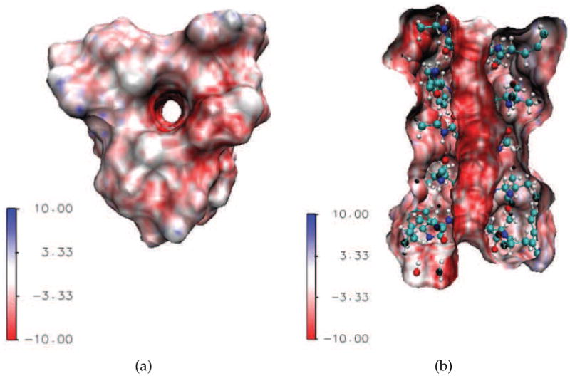
3D illustration of the Gramicidin A (GA) channel structure and surface electrostatic potential, with unit of k_BT/q. The negative surface electrostatics as indicated by the intensive red color on the channel upper surface and inside the channel pore implies that the GA selects positive ions. (a) Top view of the GA channel; (b) Side view of the GA channel.

4.1 Electrostatic properties of the Gramicidin A channel

This subsection presents the electrostatic analysis of the GA channel over a wide range of ∊(r) values in the present model. We carefully test the effect of dielectric constants within an appropriate biological range in order to obtain a reasonable prediction. It is also worth checking the dependence or changing trend of the electrostatics upon these parameters for model training and validity verification. Before the transport problem is simulated, the mathematical algorithms, choices of dielectric constants are carefully examined via the generalized Poisson-Boltzmann equation.

The electrostatics of the channel system depends on the dielectric constants. In the present work, we carefully test the effect of dielectric constants within an appropriate biological range in order to obtain a reasonable prediction. It is also worth checking the dependence or changing trend of the electrostatics upon these parameters for model training and validity verification. Before the transport problem is simulated, the mathematical algorithms, choices of dielectric constants are carefully examined via the generalized Poisson-Boltzmann equation.

As discussed earlier, ∊_m(r) is given as a constant in Ω_m and its value is tested over a range. However, ∊_s (r) is strongly position dependent, having different values in the bulk solvent and the channel pore. Although it is easy to define such a smooth function for ∊_s (r) because of the small and simple bath/channel interface, we just take ∊_s (r) as piece-wise constants for simplicity, i.e., impose a constant value denoted as ∊_bath in the bulk solvent, whereas another for the channel pore denoted as ∊_ch. There is no controversy upon the choice of ∊_bath = 80, which is employed in all the following simulations. Figs. 4-6 display the electrostatic potential profiles and (positive) ion density in GA protein with various combinations of ∊_ch and ∊_m within the range discussed in the earlier section. The reference ion density is taken as 0.1 molar.

Figure 4.

Electrostatic potential and charge density of the GA channel along the z-axis obtained with ∊_m = 2 and $n_p^0=0.1$ molar (Red: ∊_ch = 20; Green: ∊_ch = 40; Blue: ∊_ch = 80). (a) Electrostatic potential profiles in channel; (b) Proton density profiles in the channel.

Figure 6.

Electrostatic potential and charge density of the GA channel along the z-axis obtained with ∊_m = 10 and $n_p^0=0.1$ molar (Red: ∊_ch = 20; Green: ∊_ch = 40; Blue: ∊_ch = 80). (a) Electrostatic potential profiles in the channel; (b) Proton density profiles in the channel.

All quantities in Figs. 4-6 are averaged on each cross section along the channel axis. The vertical dash lines in these figures indicate the entrance (left) and exit (right) of the channel. The GA protein is overall neutral in charge, but possesses a negative environment in the channel region and this fact leads to potential well. Near the entrance and the exit of the channel, there are two local potential minima (the valley near the dash line) and a major barrier in the middle of the channel. Accordingly, for the density profile, there are two peaks at the positions where two energy minima present and the density is lower in the middle of the channel. These electrostatic profiles agree with the biological properties of the GA channel.

For each fixed ∊_m, the magnitude of the electrostatic potentials responds directly to the change of ∊_ch value, as showed in Fig. 4(a). When the ∊_ch decreases from 80, which is the commonly used value for the solvent, to the lower values suggested by biological observations, the contrast between the energy wells near the entrance/exit and the barrier in the middle becomes sharper. This phenomenon verifies the impact of ∊_ch value and leads us to prefer the lower value in our model. For the ion density profile shown in Fig. 4(b), the changes in the peaks with respect to the changes of ∊_ch are very clear. As ∊_ch doubles, the magnitudes of the density at the peaks decrease half accordingly.

The impact of ∊_m can be examined by fixing ∊_ch, i.e., checking the same color curves throughout Figs. 4-6. It can be found out that changes in ∊_m do not affect the potential structure but solely change the magnitudes. When ∊_m increases, the absolute value of electrostatic potential decreases, and consequently the proton density becomes smaller.

It is worthwhile to point out that the high ionic density calculated in the channel region is in a local sense. When the electrostatics is intensively negative at a point, by the Boltzmann distribution, the density will be very high at that position. This implies the ability of negative potential in attracting the cation. In order to obtain the physically and biologically meaningful quantities, such as dielectric constants for each region, it is useful to compare through Figs. 4–6 to seek for appropriate parameters. Actually, by comparing to experimental data, some parameters that result in extreme values of quantities, for example, the dielectric constant 20 in the channel region that corresponds very high local ionic density, are avoided in our simulation.

Fig. 7 depicts the electrostatics profile change with respect to reference proton densi­ties at a certain combination of dielectric constants (∊_m = 5 and ∊_ch =40). It is easy to see that the higher the proton reference concentration, the higher the sources in the Poisson equation and the results in electrostatic potential profiles are.

Figure 7.

Electrostatic potential profiles of the GA channel under different ion reference densities $n_p^0$. Red: $n_p^0=0.1$ molar; Green: $n_p^0=0.2$ molar; Blue: $n_p^0=1.0$ molar; Black: $n_p^0=2.0$ molar. ∊_m = 5 and ∊_ch = 40.

4.2 Proton transport efficiency in the Gramicidin A channel

The selectivity of the GA channel to cations can be easily explained in view of the overall potential landscape. Fig. 8 shows the total effective potential with both the electrostatic and generalized-correlation contributions. Fig. 8(a) is for the monovalent cations while Fig. 8(b) is for monovalent anions. According to the previous discussion, the generalized-correlation potential serves as an energy barrier while the GA protein provides a negatively charged environment for cations in the channel region. Two energy components with opposite signs cancel each other and result in an overall potential landscape that permeates a monovalent cation. However, the overall potential gives rise to a huge barrier for the anions since the positive generalized-correlation potential adds up with the positive electrostatic potential, as Fig. 8(b) shows.

Figure 8.

The total potential of the GA channel which includes electrostatic and generalized-correlation contributions under various voltage biases. Dielectric constants are ∊_m = 5 and ∊_ch = 30. The pH value of the solution is 2.75. (a) Total potential of monovalent cations; (b) Total potential of monovalent anions.

Conductance reveals the efficiency of the proton transport through the GA. Due to the fast development of experimental technologies in the past several decades, the single-channel conductance can be measured and becomes one of the prevalent descriptor of the channel function. The simulation of channel conductance mainly focuses on calculating the channel current within the physiological ranges of membrane potentials (i.e., −0.2V < V < 0.2V) and bath concentrations (up to molars). The proton transport current is measured at the scale of pico-Ampere (pA). The corresponding characteristics of channel conductance is observed at the scale of pico-Siemens (pS) and is recorded in the voltage-current (I-V) curves and concentration-current (C-C) curves. Based on experimental observations, the I-V curves are expected to be in linear or sub-linear form while the C-C curves are supposed to exhibit saturation behavior, i.e., when the concentration increases, the conductance increases linearly at beginning and then becomes saturated later on.

The efficiency of proton transport mainly depends on the proton scattering process. Thus we first present the effective potential profile along the transport direction. Fig. 9 depicts the first 15 effective potential eigenvalues (i.e., U^j(z) in Eq. (3.3)) used in the current calculation under the voltage bias of 0.2V Similarly, the channel region is presented between two black dash lines. The channel region is essentially confined by the protein surface and a tube-like pore is formed. As displayed in Fig. 9, the potential energy profile in the channel pore region has discrete eigenstates, due to the small area confinement at each cross section and the light mass of the proton. For each specific location along the transport direction, the discrete ascending energies correspond to the eigenvalues of the operator in Eq. (3.2). In theory, the total number of the eigenvalues is infinite, but is finite in practical computations, and depends on the discretization of the cross section. In principle, all the eigenvalues should be accounted in computations. However, numerically, due to the Boltzmann distribution, higher energy components contribute little in the total transport quantity. In practise, only a few low lying eigenvalues need to be included in numerical simulations. In our case, the first 15 eigenstates are sufficient to obtain a good degree of convergence in calculating the proton density and current.

Figure 9.

The first 15 eigenvalues (the U^j(z) in Eq. (3.3)) of the effective potentials along the transport direction used in the transport calculations at the voltage bias of 0.2V.

Fig. 10 illustrates the simulation results of the present multiscale model for proton transport, compared with the experimental data from the literature [40] for the GA channel. The blue dots in each figure represent the available experimental observations for certain voltage biases while the red curves are our model predictions calculated with sufficiently many voltage samples. The model parameters are chosen to match the experimental data but all choices are taken within the range of physical measurements. The dielectric coefficients are taken as ∊_m = 5, ∊_ch = 30 and ∊_bath = 80, according to the discussion in previous sections. To determine the generalized correlations, the diffusion coefficients of protons are taken as 3.6 × 10⁻⁹ m²/s in the channel, less than a half of the value in the bulk environment, and the relative weighting parameter is set to α = 0.227. Taking into account above considerations, we can conclude that experimental data and the present predictions agree quite well and this agreement verifies the validity of our quantum dynamics in continuum model.

Figure 10.

Voltage-current relation of proton translocation of GA at different concentrations. Blue dots: experimental data of Eisenman et al [25]; Red curve: model prediction.

Apart from I-V curves, there are also experimental data available about the conductance-concentration relation (C-C curve) of the proton transport under given voltages [25]. Fig. 11 displays such a relationship with a comparison between experimental data and model predictions. At a given voltage bias, the conductance of the channel is calculated with various proton concentrations as indicated by the horizontal axis. Using the same set of parameters as those in Fig. 10, the computed conductance-concentration relation also agrees fairly well with experimental data. At lower proton concentrations (i.e., pH value being greater than 2), the agreement between our prediction and experimental data is quite good. At relatively higher concentrations, although the numerical simulations slightly overestimate the observed conductance, the conductance saturation against the concentration can still be observed in simulations and it corresponds to the sub-linear characteristics or the flat tail of the C-C curve.

Figure 11.

Conductance-concentration relation of proton translocation at a fixed voltage. Voltage bias=0.05V; Blue dots: experimental data of Eisenman et al [25]; Red curve: model prediction.

The experimental data used in this work are reported by Eisenman et al [25] and are also employed to verify another proton transport model by Schumaker et al. [40]. There are other experimental data on proton conductance available [1,13,18] but under different experimental conditions. First, the experimental data provided by Cukierman et al. [18] offer proton conductions recorded with natural Gramicidin A and with its Dioxolane-Linked dimer in different lipid bi-layers (phosphatidylethanolamine-phosphatidylcholine, or PEPC and glycerymonooleate, or GMO). Their experimental studies were carried out for low (9.8 mM) and high (1578 mM) proton concentrations against the transmembrane voltages. Additionally, in another piece of work [13], the attenuation of proton transfer in Gramicidin water wires by phosphoethanolamine was investigated and a number of I-V curves were provided. It is impossible to fit all the experimental data by a single group of parameters because of the difference in experimental conditions and lipid membrane types. Nevertheless, it can be observed that our simulation curves under the current set of parameters have shown similar qualitative shapes. Therefore, the present model can fit to these experimental data by slightly adjusting model parameters to reflect the different experimental conditions. Finally, Akeson and Deamer [1] also reported I-V curves of proton conductance for the F1F0ATPases studies. In their results, a severe saturating or sublinear character is found for proton concentration of 10 mM and there was an obvious superlinear pattern for 1.0 M hydrogen chloride (HCl). Our model can not capture these characteristics by just tuning the parameter values. In fact, this set of experimental data was also found difficult for another theoretical model of proton transport [40].

4.3 Model limitations

Based on the multi-scale approximation, the present model captures the most important factors which have large impacts on the proton permeation through membrane proteins. Meanwhile, the quantum treatment of protons provides a potential analysis tool to take into account the quantum behavior in proton transport and proton translocation in biomolecules. The setup of the present model roots from essential biophysical principles with reasonable approximations, and thus the numerical simulations give considerably good agreements with experimental data under appropriate choices of model param­eters. However, this model also has a number of limitations, which are to be studied further in the future. First, in this model, the channel protein is assumed to be rigid, i.e. it does not response to the permeation of ions. This is not true in real situation and the configurational change of the channel protein has been found to have fairly important impact on the ion permeation process. Although the omitted ion-protein interaction has been somehow compensated implicitly by adjusting the dielectric constants, this interaction can not be fully accounted unless more sophisticated models, such as the multiscale molecular dynamics [43], are invoked. Additionally, the plasma membrane where the channel protein is embedded is simplified. There are various types of membranes, some of them have dipoles and others have charges. In our model, the membrane is just approximated by the uniformly distributed dielectric medium and the charges or dipole effects are neglected. However, there is no essential difficulty to improve this aspect in our model. Point charges from membranes can be added in the present model. Otherwise, a position dependent dielectric constants for the biomolecular region can also represent the charge effects in the membrane. Moreover, a fix solvent-solute interface, the molecular surface, is assumed in the present work. It is important to incorporate the variational solvent-solute interface in multiscale models and handle solvent-solute interactions [11, 43]. This aspect will be conisdered eslewhere [8]. Finally, the other limitation of the present model is the simplified local density approximation of generalized correlations, which reduces the number of the degrees of freedom, although. Compared to the electrostatic potential, the generalized-correlation potential plays a less important role in general. However, it may be of crucial importance for channel selectivity in certain situations. Therefore, an emergent task of our future work is to come up with more quantitative modeling of generalized-correlation interactions meanwhile without significantly increasing the number of degrees of freedom. Local spin density approximation, local density gradient approximation and general linear scaling approaches are under our consideration.

5 Conclusion

Proton dynamics and transport across membrane proteins are of paramount importance to the normal function of living cells. Although there are a variety of excellent theoretical models and efficient computational methods for ion channels in general, most commonly used models are much less successful when they are applied to the proton transport due to the unique characteristics of protons. It is commonly believed that to a certain extent, proton transport through narrow channel pore demonstrates quantum mechanical properties such as the translocation as shown in the Grotthuss-type mechanism [33]. However, the exact role of quantum mechanics in the atomic mechanism of proton transport is still unclear despite of a number of elegant theories in the literature, partly due to the complexity of ion channel systems. The present paper introduces a quantum dynamics in continuum (QDC) model for the prediction and analysis of proton density distribution and conductance in proton transport. Our essential ideas are as follows. First, protons behave quantum mechanically due to their light masses and channel geometric confinement in protein channels. Therefore, a quantum mechanical treatment of protons is necessary. Additionally, since the primary interactions in proton transport through membrane proteins are of ion-ion electrostatic type and the van der Waals type of interactions involve less energy, a dielectric continuum treatment of solvent medium may provide a reasonable approximation to the effect of numerous solvent molecules. Most importantly, this treatment dramatically reduces the dimensionality of the problem. As such, our approach is called a QDC model. Moreover, since the atomic detail of the protein structure serves as a physical boundary for proton dynamics and transport, the present model returns molecular surface to separate the continuum solvent domain from the discrete charge domain of the protein. Finally, densities of all other ions and counterions in the solvent are described by the Boltzmann distribution, which is a quasi-equilibrium description as the electrostatic potential varies during the process of protons permeating the membrane.

We propose a multiscale variational paradigm to accommodate the aforementioned aspects in a unified framework. The total free energy functional encompasses the kinetic and potential energies of protons, and the electrostatic energies of ions and fixed charges in the channel system. The first variation is carried out via the Euler-Lagrange equation to derive the governing equations for the system. A generalized Poisson-Boltzmann equation is obtained for the electrostatic potential while a generalized Kohn-Sham equation is resulted for the state of protons in the system. The solution to these two coupled nonlinear equations leads to the desirable electrostatic distribution and proton density profile in the channel system. Expressions for proton density and proton flux across the membrane are derived from fundamental principles.

The computation of the proposed coupled equations involves a number of mathematical issues, such as the linearization of coupled nonlinear partial differential equations (PDEs) using the Gummel iterations and/or inexact Newton iterations, and the solution of elliptic PDEs with discontinuous coefficients (i.e., piecewise dielectric constants), singular sources (i.e., Dirac delta functions for protein charges), and nonsmooth interfaces (i.e., geometric singularities). In the present work, we utilize the Dirichlet to Neumann mapping method to take care of singular charges, and the matched interface and boundary (MIB) method to accurately handle the discontinuous coefficients and geometric singularities.

The Gramicidin A (GA) channel protein, a popular protein structure, is employed in our numerical studies to demonstrate the performance of the proposed QDC model. We give a detailed discussion about the rational for model parameter selections. The electrostatic property of the GA channel is analyzed with the proposed model against a large number of model parameters. Proton transport properties, i.e., the current voltage (I-V) curves, are investigated over a large number of combinations of applied voltages and reference bulk concentrations. Our simulation predictions are compared with experimental data, which validates the present QDC model. Finally, we provide detailed discussion of model limitations and possible future improvements.

Figure 5.

Electrostatic potential and charge density of the GA channel along the z-axis obtained with ∊_m=5 and $n_p^0=0.1$ molar (Red: ∊_ch = 20; Green: ∊_ch = 40; Blue: ∊_ch = 80). (a) Electrostatic potential profiles in the channel; (b) Proton density profiles in the channel.

References

- 1.Akeson M, Deamer D. Proton conductance by the gramicidin water wire. Model for proton conductance in the F0F1ATPases? Biophys J. 1991;60:101–109. doi: 10.1016/S0006-3495(91)82034-3. [DOI] [PMC free article] [PubMed] [Google Scholar]
- 2.Bernal J, Fowler R. A theory of water and ionic solution, with particular reference to hydrogen and hydroxyl ions. J Chem Phys. 1933;1:515–548. [Google Scholar]
- 3.Bothma J, Gilmore J, McKenzie R. The role of quantum effects in proton transfer reactions in enzymes: Quantum tunneling in a noisy environment? New J Phys. 2010;12(055002) [Google Scholar]
- 4.Brandsburg-zabary S, Fried O, Marantz Y, Nachliel E, Gutman M. Biophysical aspects of intra-protein proton transfer. Biochim Biophys Acta. 2000;1458:120–134. doi: 10.1016/s0005-2728(00)00063-3. [DOI] [PubMed] [Google Scholar]
- 5.Braun-Sand S, Burykin A, Chu ZT, Warshel A. Realistic simulations of proton transport along the gramicidin channel: Demonstrating the importance of solvation effects. J Phys Chem B. 2005;109:583–592. doi: 10.1021/jp0465783. [DOI] [PubMed] [Google Scholar]
- 6.Breed J, Sankararamakrishnan R, ID K, Sansom M. Molecular dynamics simulations of water within models of ion channels. Biophys J. 1996;70:1643–1661. doi: 10.1016/S0006-3495(96)79727-8. [DOI] [PMC free article] [PubMed] [Google Scholar]
- 7.Chen D, Chen Z, Chen CJ, Geng WH, Wei GW. MIBPB: A software package for electrostatic analysis. J Comput Chem. 2011;32:657–670. doi: 10.1002/jcc.21646. [DOI] [PMC free article] [PubMed] [Google Scholar]
- 8.Chen D, Chen Z, Wei GW. Quantum dynamics in continuum for proton transport II: Variational solvent-solute intersurface. Int J Numer Methods Biomed Engr. 2012;28:25–51. doi: 10.1002/cnm.1458. [DOI] [PMC free article] [PubMed] [Google Scholar]
- 9.Chen D, Lear J, Eisenberg B. Permeation through an open channel: Poisson-Nernst-Planck theory of a synthetic ionic channel. Biophys J. 1997;72(1):97–116. doi: 10.1016/S0006-3495(97)78650-8. [DOI] [PMC free article] [PubMed] [Google Scholar]
- 10.Chen D, Wei GW. Modeling and simulation of electronic structure, material interface and random doping in nano-electronic devices. J Comput Phys. 2010;229:4431–4460. doi: 10.1016/j.jcp.2010.02.002. [DOI] [PMC free article] [PubMed] [Google Scholar]
- 11.Chen Z, Baker NA, Wei GW. Differential geometry based solvation models I: Eulerian formulation. J Comput Phys. 2010;229:8231–8258. doi: 10.1016/j.jcp.2010.06.036. [DOI] [PMC free article] [PubMed] [Google Scholar]
- 12.Chen Z, Baker NA, Wei GW. Differential geometry based solvation models II: Lagrangian formulation. J Math Biol. 2011 doi: 10.1007/s00285–011–0402–z. pages. [DOI] [PMC free article] [PubMed] [Google Scholar]
- 13.Chernyshev A, Cukierman S. Proton transfer in gramicidin water wires in phosphlipid bilayers: Attenuation by phosphoethanolamine. Biophys J. 1997;91:580–587. doi: 10.1529/biophysj.106.083352. [DOI] [PMC free article] [PubMed] [Google Scholar]
- 14.Chung SH, Allen T, Kuyucak S. Conducting-state properties of the KcsA potassium channel from molecular and Brownian dynamics simulations. Biophys J. 2002;82:628–645. doi: 10.1016/S0006-3495(02)75427-1. [DOI] [PMC free article] [PubMed] [Google Scholar]
- 15.Chung SH, Kuyucak S. Recent advances in ion channel research. Biochimica et Biophysica Acta. 2002;1565:267–286. doi: 10.1016/s0005-2736(02)00574-6. [DOI] [PubMed] [Google Scholar]
- 16.Coalson RD, Kurnikova MG. Poisson-Nernst-Planck theory approach to the calculation of current through biological ion channels. IEEE Trans Nanobioscience. 2005;4(1):81–93. doi: 10.1109/tnb.2004.842495. [DOI] [PubMed] [Google Scholar]
- 17.Cukier R. Theory and simulation of proton-coupled electron transfer, hydrogen-atom transfer, and proton translocation in proteins. Biochimica et Biophysical Acta-Bioenergetics. 2004;1655:37–44. doi: 10.1016/j.bbabio.2003.06.011. [DOI] [PubMed] [Google Scholar]
- 18.Cukierman S, Quigley EP, Crumrine DS. Proton conduction in Gramicidin A and in its dioxolane-linked dimer in different lipid bilayers. Biophys J. 1997;73:2489–2502. doi: 10.1016/S0006-3495(97)78277-8. [DOI] [PMC free article] [PubMed] [Google Scholar]
- 19.de Falco C, Jerome JW, Sacco R. A self-consitent iterative scheme for the one-dimensional steady-state transistor calculations. IEEE Trans Ele Dev. 1964;11:455–465. [Google Scholar]
- 20.Decoursey T. Voltage-gated proton channels and other proton transfer pathways. Physiol Rev. 2003;83:475–579. doi: 10.1152/physrev.00028.2002. [DOI] [PubMed] [Google Scholar]
- 21.Dolinsky TJ, Nielsen JE, McCammon JA, Baker NA. PDB2PQR: An automated pipeline for the setup, execution, and analysis of Poisson-Boltzmann electrostatics calculations. Nucleic Acids Research. 2004;32:W665–W667. doi: 10.1093/nar/gkh381. [DOI] [PMC free article] [PubMed] [Google Scholar]
- 22.Dunker A, Marvin D. A model for membrane transport through α-helical protein pores. J Theor Biol. 1978;72:9–16. doi: 10.1016/0022-5193(78)90015-2. [DOI] [PubMed] [Google Scholar]
- 23.Deamer DW. Intracellular pH: Its Measurement, Regulation, and Utilization in Cellular Functions. New York: Liss; 1982. Proton permeability in biological and model membranes. [Google Scholar]
- 24.Edwards S, Corry B, Kuyucak S, Chung SH. Continuum electrostatics fails to describe ion permeation in the gramicidin channel. Biophys J. 2002 Sep;83:1348–1360. doi: 10.1016/S0006-3495(02)73905-2. [DOI] [PMC free article] [PubMed] [Google Scholar]
- 25.Eisenman G, Enos B, Hagglund J, Sandbloom J. Gramicidin as an example of a single-filing ion channel. Ann N Y Acad Sci. 1980;339:8–20. doi: 10.1111/j.1749-6632.1980.tb15964.x. [DOI] [PubMed] [Google Scholar]
- 26.Geng WH, Yu SN, Wei GW. Treatment of charge singularities in implicit solvent models. J Chem Phys. 2007;127:114106. doi: 10.1063/1.2768064. [DOI] [PubMed] [Google Scholar]
- 27.Gilson MK, Davis ME, Luty BA, McCammon JA. Computation of electrostatic forces on solvated molecules using the Poisson-Boltzmann equation. J Phys Chem. 1993;97(14):3591–3600. [Google Scholar]
- 28.Krishtalik L. The mechanism of the proton transfer: An outline. Biochimica et Biophysical Acta-Bioenergetics. 2000;1458:6–27. doi: 10.1016/s0005-2728(00)00057-8. [DOI] [PubMed] [Google Scholar]
- 29.Kuyucak S, Andersen OS, Chung SH. Models of permeation in ion channels. Rep Prog Phys. 2001;64:1427–1472. [Google Scholar]
- 30.MacKerell AD, J, Bashford D, Bellot M, Dunbrack RL, J, Evanseck JD, Field MJ, Fischer S, Gao J, Guo H, Ha S, Joseph-McCarthy D, Kuchnir L, Kuczera K, Lau FTK, Mattos C, Michnick S, Ngo T, Nguyen DT, Prodhom B, Reiher WE, I, Roux B, Schlenkrich M, Smith JC, Stote R, Straub J, Watanabe M, Wiorkiewicz-Kuczera J, Yin D, Karplus M. All-atom empirical potential for molecular modeling and dynamics studies of proteins. J Phys Chem B. 1998;102(18):3586–3616. doi: 10.1021/jp973084f. [DOI] [PubMed] [Google Scholar]
- 31.Mamonov AB, Coalson RD, Nitzan A, Kurnikova MG. The role of the dielectric barrier in narrow biological channels: A novel composite approach to modeling single-channel currents. Biophys J. 2003 Jun;84:3646–3661. doi: 10.1016/S0006-3495(03)75095-4. [DOI] [PMC free article] [PubMed] [Google Scholar]
- 32.Mitchell P. Vectorial chemistry and the molecular mechanics of chemiosmotic coupling: power transmission by proticity. Biochem Soc Trans. 1976;4:399–430. doi: 10.1042/bst0040399. [DOI] [PubMed] [Google Scholar]
- 33.Nagle J, Morowitz H. Molecular mechanisms for proton transport in membranes. Proc Natl Acad Sci U S A. 1978;1458(72):298–302. doi: 10.1073/pnas.75.1.298. [DOI] [PMC free article] [PubMed] [Google Scholar]
- 34.Perlman D, Case D, Caldwell J, Ross W, Cheatham T, Debolt S, Ferguson D, Seibel G, Kollman P. Amber, a package of computer programs for applying molecular mechanics, normal mode analysis, molecular dynamics and free energy calculations to simulate the structural and energetic properties of molecules. Comp Phys Commun. 1995;91:1–41. [Google Scholar]
- 35.Pomes R, Roux B. Structure and dynamics of a proton wire: A theoretical study of H+ translocation along the single-file water chain in the Gramicidin A channel. Biophys J. 2002;71:19–39. doi: 10.1016/S0006-3495(96)79211-1. [DOI] [PMC free article] [PubMed] [Google Scholar]
- 36.Roux B. Influence of the membrane potential on the free energy of an intrinsic protein. Biophys J. 1997 Dec;73:2980–2989. doi: 10.1016/S0006-3495(97)78327-9. [DOI] [PMC free article] [PubMed] [Google Scholar]
- 37.Sanner MF, Olson AJ, Spehner JC. Reduced surface: An efficient way to compute molecular surfaces. Biopolymers. 1996;38:305–320. doi: 10.1002/(SICI)1097-0282(199603)38:3%3C305::AID-BIP4%3E3.0.CO;2-Y. [DOI] [PubMed] [Google Scholar]
- 38.Sansom M, Kerr I, J Breed, Sankararamakrishnan R. Water in channel-like cavities: Structure and dynamics. Biophys J. 1996;70:693–702. doi: 10.1016/S0006-3495(96)79609-1. [DOI] [PMC free article] [PubMed] [Google Scholar]
- 39.Schnell JR, Chou JJ. Structure and mechanism of the M2 proton channel of influenza A virus. Nature. 2008 Jan;451:591–596. doi: 10.1038/nature06531. [DOI] [PMC free article] [PubMed] [Google Scholar]
- 40.Schumaker MF, Pomes R, Roux B. A combined molecular dynamics and diffusion model of single proton conduction through gramicidin. Biophys J. 2000 Dec;79:2840–2857. doi: 10.1016/S0006-3495(00)76522-2. [DOI] [PMC free article] [PubMed] [Google Scholar]
- 41.Sharp KA, Honig B. Electrostatic interactions in macromolecules – Theory and applications. Annual Review of Biophysics and Biophysical Chemistry. 1990;19:301–332. doi: 10.1146/annurev.bb.19.060190.001505. [DOI] [PubMed] [Google Scholar]
- 42.Till MS, Essigke T, Becker T, Ullmann GM. Simulating the proton transfer in Gramicidin A by a sequential dynamical Monte Carlo method. J Phys Chem. 2008;112:13401–13410. doi: 10.1021/jp801477b. [DOI] [PubMed] [Google Scholar]
- 43.Wei GW. Differential geometry based multiscale models. Bulletin of Mathematical Biology. 2010;72:1562–1622. doi: 10.1007/s11538-010-9511-x. [DOI] [PMC free article] [PubMed] [Google Scholar]
- 44.Yu SN, Wei GW. Three-dimensional matched interface and boundary (MIB) method for treating geometric singularities. J Comput Phys. 2007;227:602–632. [Google Scholar]
- 45.Yu SN, Zhou YC, Wei GW. Matched interface and boundary (MIB) method for elliptic problems with sharp-edged interfaces. J Comput Phys. 2007;224(2):729–756. [Google Scholar]
- 46.Zheng Q, Chen D, Wei GW. Second-order Poisson-Nernst-Planck solver for ion transport. J Comput Phys. 2011;230:5239–5262. doi: 10.1016/j.jcp.2011.03.020. [DOI] [PMC free article] [PubMed] [Google Scholar]
- 47.Zheng Q, Wei GW. Poisson-Boltzmann-Nernst-Planck model. J Chem Phys. 2011;134:194101. doi: 10.1063/1.3581031. [DOI] [PMC free article] [PubMed] [Google Scholar]
- 48.Zhou YC, Feig M, Wei GW. Highly accurate biomolecular electrostatics in continuum dielectric environments. J Comput Chem. 2008;29:87–97. doi: 10.1002/jcc.20769. [DOI] [PubMed] [Google Scholar]
- 49.Zhou YC, Wei GW. On the fictitious-domain and interpolation formulations of the matched interface and boundary (MIB) method. J Comput Phys. 2006;219(1):228–246. [Google Scholar]
- 50.Zhou YC, Zhao S, Feig M, Wei GW. High order matched interface and boundary method for elliptic equations with discontinuous coefficients and singular sources. J Comput Phys. 2006;213(1):1–30. [Google Scholar]