Hierarchical model of natural images and the origin of scale invariance

Abstract

The study of natural images and how our brain processes them has been an area of intense research in neuroscience, psychology, and computer science. We introduced a unique approach to studying natural images by decomposing images into a hierarchy of layers at different logarithmic intensity scales and mapping them to a quasi-2D magnet. The layers were in different phases: “cold” and ordered at large-intensity scales, “hot” and disordered at small-intensity scales, and going through a second-order phase transition at intermediate scales. There was a single “critical” layer in the hierarchy that exhibited long-range correlation similar to that found in the 2D Ising model of ferromagnetism at the critical temperature. We also determined the interactions between layers mapped from natural images and found mutual inhibition that generated locally “frustrated” antiferromagnetic states. Almost all information in natural images was concentrated in a few layers near the phase transition, which has biological implications and also points to the hierarchical origin of scale invariance in natural images.

Our visual system evolved to survive in nature with scenes of mountains, rivers, trees, and other animals (1). The neural representations of visual inputs are related to their statistical structure (1–3). Structures in nature come in a hierarchy of sizes that cannot be separated, a signature of scale invariance, which also occurs near a critical point in many physical systems. The classic example of a critical point is a uniaxial ferromagnetic system going through a second-order phase transition in a zero magnetic field by increasing temperature. At the critical point, the system loses its magnetization due to thermal fluctuations. There are large regions (“islands”) that are magnetized in one direction but are surrounded by large regions (“seas”) that are magnetized in the opposite direction. The seas themselves are embedded in bigger islands, ad infinitum. The total magnetization is zero, but the correlation length diverges, which is visualized by growth of the sizes of seas and islands with the system size. At the critical point, the system is free of a length scale because fluctuations occur at scales of all lengths. The infinite correlation length is thus intricately linked with scale invariance. The scale invariance in natural images was first characterized by the 1/f² spatial power spectrum of pixel intensities (2). Here, we study scaling properties of natural images at a deeper level by finding a hierarchy of statistical structures, in which the scale invariance emerges near a second-order phase transition.

Images are preprocessed in the retina by a complex network with ∼55 distinct cell types in mammals (5). The cerebral cortex receives a spatiotemporal stream of spikes that contain all the information in the visual inputs that has been coded by the retina. Understanding the hierarchies of statistical structures in natural images is essential for better understanding how that information is efficiently encoded by the retina. This might also yield insights into how the cortex represents scale-invariant visual scenes.

Mental imagery suggests that the brain has developed generative models of sensory experiences. Generative models, such as the Boltzmann machine, have been used to represent the statistical structure of images (6–8). Here we develop a unique input representation for images in which the lateral interactions in the input representation of the Boltzmann machine are learned from natural images.

Results

Image Representation.

For simplicity, consider gray-scaled images, and with no loss of generality, assume the image intensities are nonnegative integers, represented by the matrix ℐ. The intensity matrix therefore can be written uniquely as the weighted sum of matrices ℬ^λ:

where the integer b > 1 is the base of the representation, ℬ^λ are nonnegative integer matrices with values between 0 and b − 1, and L is the length of the representation. ℬ^λ is found iteratively by calculating starting from λ = 1, where ⌊⋅⌋ is the floor function. Similar to base representation of integers, we can think of the ordered collection of matrices (ℬ¹ℬ²…ℬ^L) as the base b representation of the matrix ℐ. This generalizes the attempts made in studying sounds and natural images by binarizing them according to their median intensities (9, 10). We call layers ℬ^λ intensity layers in general, and binary layers for b = 2.

Phase Transition in Natural Images.

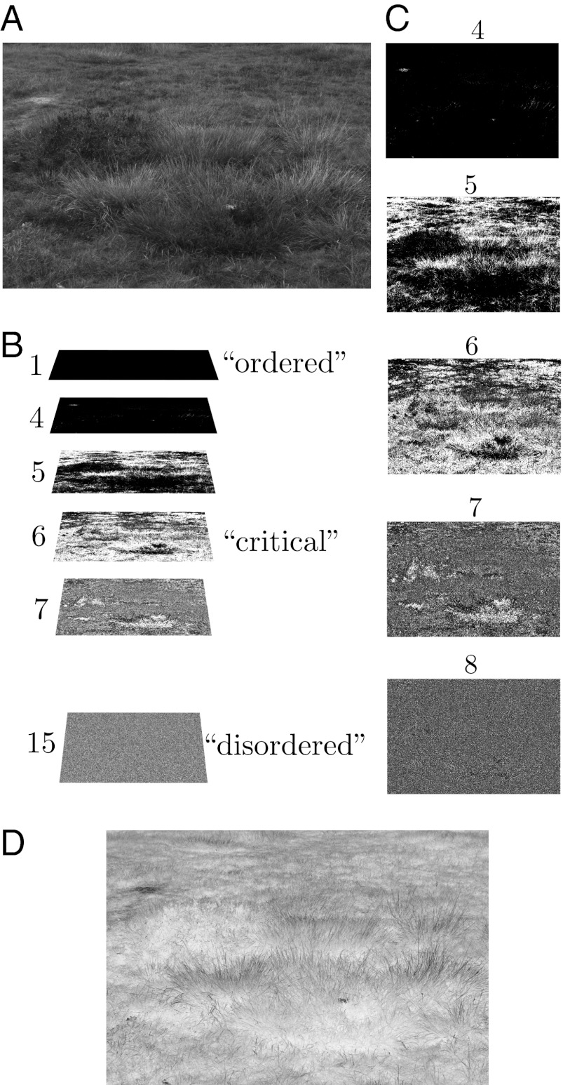
An example of an image in the van Hateren database (11) (Fig. 1A) and its binary (b = 2) decomposition (Fig. 1C) is given in Fig. 1. In that database, the maximum intensity is 2¹⁵ − 1, so L = 15 for the binary representation. Fluctuations in ℬ¹ (ℬ^L) code the largest (smallest) intensity variation, and we call it the top (bottom) layer to highlight the intensity dimension visualized in Fig. 1B. Looking at this example, one immediately notices the qualitative change moving down from the top layer to the bottom one. In physical systems, the top layer is called an ordered phase and the bottom one is called a disordered phase. The same behavior is seen for all images in the ensemble, as well as for images in other databases, including color and compressed JPEG (Joint Photographic Experts Group) images.

Fig. 1.

Visualization of the base representation of images. (A) Example of an image in the van Hateren database of natural images. It consists of 4,167 images, 1,024 × 1,536 pixels in size, ranging from 0 to 2¹⁵ − 1 in the pixel intensity. (B) In the base representation, the 2D image is isomorphic to a quasi-2D system by stacking layers ℬ^λ from top λ = 1 to bottom λ = L. Numbers denote λ, with phases for λ = 1, 6, and 15 identified. (C) Layers 4:8 from top to bottom in the binary decomposition are shown separately. The pixel intensity on each layer is either 0 (black) or 1 (white). Traces of a second-order phase transition near λ = 6 are also visualized here. Layers 1:3 and 9:15 are not shown because of space; they are indistinguishable from ordered and disordered layers 1 and 15 (shown in B), respectively. (D) This image is the “negative” representation of A, equivalent to flipping pixel values 0 ↔ 1 of the binary planes.

The ordered and disordered phases are easily explained. In a binary representation, the intensity needs to be at least 2¹⁴ for a pixel in the top layer to be active, and this occurs in only 0.02% of pixels in the van Hateren database. The origin of the disorder in the bottom layer (which codes the smallest intensity variation) can be traced back to the stochastic nature of the detection process.

The theory of second-order phase transition is well established in physics, starting with the simple and elegant Landau–Ginzburg theory (12) that led to the comprehensive machinery of the renormalization group (4). The Landau–Ginzburg theory of critical phenomena starts with a mean field formulation by introducing a macroscopic “order parameter” M, which is the average of a microscopic variable. M is the average magnetization for a uniaxial ferromagnet in a zero magnetic field, and the free energy must respect the symmetry M → −M. The first two terms in the free energy (up to a scaling factor) are given by F = rM² + M⁴ + (M⁶). At the phase transition, r changes sign from positive to negative and the minimum solution goes from zero to a nonzero value. There are two degenerate nonzero solutions, which are mapped to each other by a sign flip. However, the system has to pick one of the solutions, what is known as spontaneous symmetry breaking: The free energy is symmetrical, but the equilibrated state breaks the symmetry. In the following, we define an order parameter for layers ℬ^λ (Eq. 1 and Fig. 1). The order parameter is zero for the bottom layers, and it develops a nonzero value at an intermediate “critical” layer, becoming fully ordered at the top layer (Fig. 1B).

Mapping Images to Magnets.

Define the following “spin” variable at pixel i = (i₁, i₂) on layer λ:

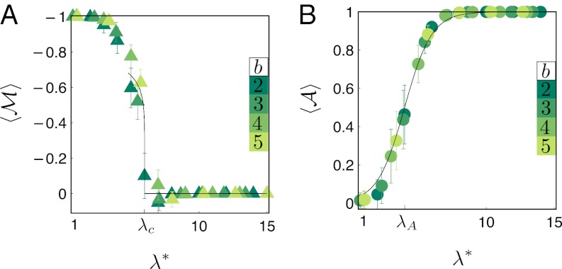
The normalization is done to limit in all bases. The “magnetization” order parameter ℳ^λ for the layer λ is then obtained by averaging over image pixels: . Looking at natural images as a statistical ensemble, the quantity of interest is 〈ℳ^λ〉, which is the average of ℳ^λ over the ensemble, plotted in Fig. 2B for different bases. If we assume λ is the tuning parameter for the phase transition, just below the critical value λ_c, the average order parameter is given by 〈ℳ〉 = (λ_c − λ)^β/C. The best fit was obtained for λ_c = 6.00, β = 0.12, and C = −1.50 (Fig. 2B). The exponent β is close to the critical exponent β = 1/8 of the 2D Ising model. One might object that the tuning parameter, λ, is not continuous here. However, this is only a practical issue because it can be made asymptotically continuous by constructing databases with a large L. We “translated” λ in different bases back to the binary b = 2 (Fig. 2), thus creating a limited continuity (away from integer values) in λ.

Fig. 2.

Second-order phase transition, the information hidden near phase transition, and the exponent β. (A) Plot of 〈ℳ〉 for b = 2–5 as a function of λ*, obtained from . The SD is indicated by the error bars. The black curve is the best fit to the points near the phase transition (λ_c = 6), with the critical exponent β = 0.12. (B) Ensemble average 〈〉 for b = 2–5 with the same procedure as in A for representing λ in base 2 denoted by λ*. It is best fit by the sigmoid function centered at λ_A = 4.

Intensity Layers and the Information Hierarchy.

Next, we constructed two dimensionless measures to characterize the information content of each isolated layer and the accumulated information moving from the top layer to the bottom layer. They are denoted by and , respectively:

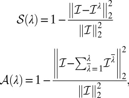where ℐ^λ = b^L−λℬ^λ is the contribution of layer λ to image ℐ given in Eq. 1, and ‖ℐ‖₂ is the Frobenius norm of the matrix ℐ. We used these measures to determine whether the most informative layers are the ones near the phase transition. The curve (λ) (not shown here) is unimodal, peaks at λ = 5, and is less than 0.2 for λ outside the interval (3, 6). In addition, the accumulated information (λ) for different bases (Fig. 2B) was best fit by the sigmoid function 1/(1 + exp(λ_A − λ)), with λ_A = 4.

Power Spectrum of Binary Layers.

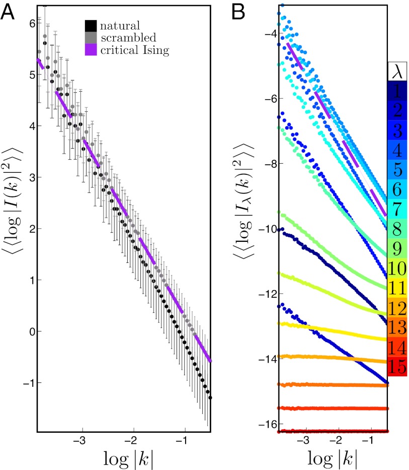
Natural images are scale-invariant (2, 13), with a correlation length of the order of the image size and with structures over a wide range of sizes. Long, smooth edges of objects induce correlation lengths on the order of the object size, and objects come in variety of sizes, which is a problem with many scales of length (4). Scale invariance and the large correlation length are quantified by studying the intensity correlation function, which shows a power law behavior in the limit of large D(i, j): 〈ℐ_iℐ_j〉 ∼ 1/D(i, j)^η, where is the distance between pixels i and j in units of pixels. In Fourier space, the scaling takes the form |I(k)|² ∼ 1/|k|^2−η as |k| → 0. For natural images, η ≃ 0 (14) (Fig. 3A). For a system with finite correlation length ξ, the correlation function decays exponentially with the characteristic length ξ. For natural images, the decay is power-law, free of a length scale, and the correlation length is “infinite.” In the framework introduced here, neither the top nor bottom layer has a large correlation length, and the infinite correlation length emerges at the phase transition. Furthermore, the exponent η for layer λ = 6 is 0.21, a substantial departure from η ≃ 0 for natural images and close to the Ising critical exponent η = 0.25. We should point out that in contrast, binarizing images by their median intensity leads to approximately the same exponent as the original image (10). The log power spectrum of layers log|I^λ(k)|² plotted in Fig. 3B compares the spectral power of each layer in isolation. Layers near the critical point contribute substantially to the power spectrum despite the fact that they have exponentially less intensity than the ordered phase. The lowest spatial frequencies are cut off because they are dominated by size effects below the cutoff. Furthermore, the power spectrum for layers away from the phase transition plateau out below the cutoff (log|k| < −4), indicating finite correlation length.

Fig. 3.

Power spectrum of binary layers, natural images, and scrambled natural images. (A) Power spectrum of natural images in black and scrambled natural images in gray. The purple dashed line is the result for the critical point of the 2D ferromagnetic Ising model. (B) Power spectrum of binary layers of natural images weighted by 2^15−λ (Iλ(k) is the Fourier transform of ℐ^λ = 2^15−λℬ^λ), from the top cold layer represented by dark blue to the hot bottom layer represented by red. The inner average is over different k orientations, and the outer average is over the ensemble of images.

Ising Model for Isolated Binary Layers.

The more direct evidence for Ising criticality is given by learning a generative model for layer λ = 6. There is a rich history for solving such a learning problem, starting with Boltzmann machines (6) and extending through recent advancements in deep belief networks (7). We used minimum probability flow learning (15) and applied it to more than 10⁶ samples (20 × 20 patches) taken from isolated layers in the binary decomposition. The program learned the Ising interactions of the fully connected network for each layer:

by assigning probability weights P({σ_i}) = exp(−E)/Z, where Z is the partition function and the temperature is absorbed in the interactions. The mean and SD of interactions with a fixed D(i, j) for layers 5, 6, and 7 are given in Table 1. For the nearest-neighbor interaction, J₁, D(i, j) = 1; for the next-nearest-neighbor interaction, J₂, (Fig. 4). We assumed translation and rotation symmetry in averaging interactions with a fixed D(i, j), consistent with the isotropy of natural images. Ignoring J_ij beyond next-nearest neighbors, the (J₁, J₂) model for layer λ = 6 is close to the phase transition of the 2D (J₁, J₂) Ising model reported in the literature: Fixing J₁ = 0.242, the estimated phase transition happens for J₂ = 0.144 (16, 17). The interactions for layers 5 and 7 correspond to the ordered and disordered phases of the Ising model, respectively. The small effective magnetic field H suggests that layer λ = 6 is slightly above the phase transition; this is due to the fact that the training was done over only positive images (Fig. 1A). If, instead, we train the network over both positive and negative (Fig. 1D) images, the same interactions (within the significant digits shown) are obtained, except for the magnetic field, which vanishes.

Table 1.

Ising interactions learned by sampling 20 × 20 patches from layers 5, 6, and 7

	λ = 5	λ = 6	λ = 7	D(i, j)
H	−0.017 ± 0.006	−0.049 ± 0.002	−0.006 ± 0.001	0
J1	0.34 ± 0.04	0.24 ± 0.04	0.16 ± 0.03	1
J2	0.14 ± 0.01	0.11 ± 0.004	0.09 ± 0.004	√2
J3	0.05 ± 0.01	0.05 ± 0.01	0.05 ± 0.01	2
J4	0.000 ± 0.007	0.004 ± 0.003	0.013 ± 0.003	√5

Ising interactions used in Eq. 2 are averaged over pairs (i, j) subjected to the distance D(i, j) given in the last column.

Fig. 4.

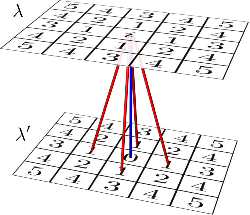
Organization of J_ij by D_⊥(i, j). The distances D_⊥(i, j) within layer λ and between λ and λ′ are ranked after fixing i on layer λ. The site labeled 0 is the site with D_⊥(i, j) = 0, the sites labeled 1 are the sites with D_⊥(i, j) = 1, and the sites labeled 2 are the sites with , etc. The site i is chosen at the center for the sake of presentation. The interaction on the blue link contributes to J₀ between layers λ and λ′, and the interactions on the red links contribute to J₁ between these two layers. The rest of the links (not shown here) are obtained by varying the site i and repeating the procedure.

The other advantage of symmetrical interactions is that we could sample smaller patches and get close to the true Ising interactions. For example, sampling 10 × 10 patches of layer 6 yields J₁ = 0.253 ± 0.044, J₂ = 0.112 ± 0.005, J₃ = 0.058 ± 0.015, and J₄ = 0.006 ± 0.003, all within the SD of the Ising interactions given in Table 1. We exploit this property in the next section. Finding similar interactions by sampling different patch sizes is a nontrivial check on the validity of minimum probability flow learning for this system. Including higher order interactions will change these numbers. However, our hypothesis is that these changes are “irrelevant” for the critical layer because interactions are coarse-grained in the renormalization group procedure (4). This is beyond the scope of the present study.

Ising Model for Connected Binary Layers.

The interactions given in Table 1 are effective interactions for each layer, that is, “effective” because each layer is sampled in isolation from other layers. We investigated interactions between layers by sampling them simultaneously and learning the Ising interactions for the fully connected network. The interactions were organized by their symmetries as in the previous section. We performed this analysis for different stack layers and patch sizes. Here, we report the results by sampling seven layers 3:9; noting that, on average, 97% of information of an image is inside layers 3:9. The learning algorithm was trained over both positive and negative images. We comment on the symmetry breaking and Monte Carlo samples elsewhere in this study (Discussion).

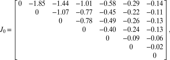
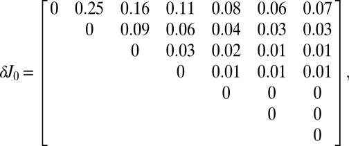
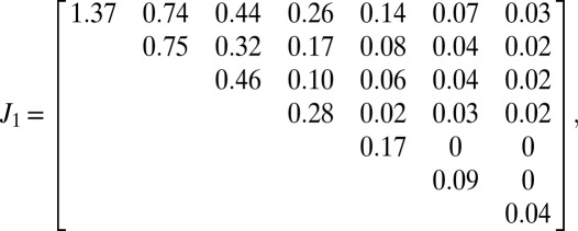
The learned Ising interactions were organized by their projection distance D_⊥(i, j) between the units i and j. The projection distance D_⊥(i, j) is related to D(i, j) through the relation , where Δλ is the vertical distance between the two sites. For example, J₀ is a 7 × 7 matrix, where the element (λ₁, λ₂) (3 ≤ λ ≤ 9) is the direct vertical interaction between layers λ₁ and λ₂, which is calculated by averaging the Ising interactions between units i and j on layers λ₁ and λ₂ subjected to D_⊥(i, j) = 0 (blue links in Fig. 4). The same procedure is performed by restricting D_⊥(i, j) = 1 (red links in Fig. 4) to obtain J₁. The Ising interactions were learned by sampling 10 × 10 patches, with 100 samples per image (416,700 samples in total). The upper triangular part of the symmetrical 7 × 7 matrices J₀, J₁ and the corresponding SD of the averaged interactions δJ₀, δJ₁ are given below:

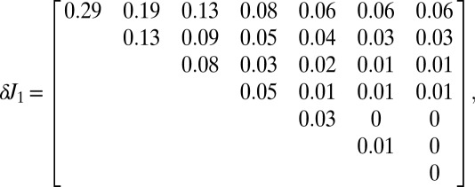where interactions smaller than 0.01 are set to 0. The significant nontrivial observation is the antiferromagnetic (inhibitory) interactions between units with vertical connections between different layers, given by J₀. The antiferromagnetic interactions are nontrivial because they are “frustrated,” a term used in magnetism literature to describe Ising interactions in which the simultaneous minimization of the interaction energies for all connections is impossible. Implications of the frustrated antiferromagnetic interactions between layers will be the subject of further studies.

Scrambled Natural Images.

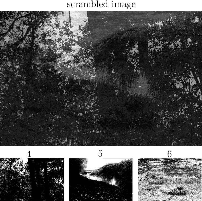
We also studied the power spectrum for a unique class of images that are easily constructed from the base decomposition. We call this class scrambled natural images. It is constructed by pooling ℬ^λ values at random from different images and combining them using Eq. 1. The layers in scrambled images are therefore independent. An example is shown in Fig. 5, with layer 6 taken from the example of Fig. 1. The linear fit to the log power spectrum of scrambled natural images yields η_scrambled = 0.14 (Fig. 3A). A general property of scrambled images, displayed in Fig. 5, is that they show structures of the informative layers at different intensity scales. The exponent η is defined by the behavior of the correlation function at large distances (small spatial frequencies). However, as is seen in Fig. 3, in the intermediate regimes, the correlation function of scrambled images matches the Ising critical system. This is due to the fact that most of the information in these images is captured by layers near the phase transition. Scrambled natural images isolate the effect of correlation between layers present in natural images. This interlayer correlation, quantified by the Ising interactions in the previous section, is the reason for the change in the slope of the power spectrum of natural images from the scrambled images. Quantifying this effect by relating it to the interlayer Ising interactions is an interesting future direction.

Fig. 5.

Scrambled natural images. The scrambled image (Upper) and the layers 4, 5, and 6 used for its construction are shown. Layer 6 is taken from the example of Fig. 1, and other layers are taken randomly from the binary decomposition of different images in the database. Layers 1:3 and 7:15 are not shown because of space; altogether, they contain only 5% of the information in this example.

Discussion

A previous analysis of natural images approximated images with a single-layer Ising model by thresholding and binarizing the pixels based on the median intensity (10). In the images we analyzed, the median intensity lies, on average, between layers 5 and 6 (5.7 ± 0.46). The binary image obtained by thresholding based on the median intensity is approximately equal to the disjunction of layers above the median layer (by applying the logical OR operator). This is approximate because the median “layer” obtained from L − log₂(median(ℐ)) is not necessarily an integer. It is likely that the criticality reported by Stephens et al. (10) has its roots in the critical “region” reported here. The change in scaling of the spectral power is due to mixing the layers with the disjunction operator. As we have shown here, extending the Ising model to multiple layers of intensities explains the scaling of natural images, can be extended to generalized (nonbinary) Ising models, and may lead to a generative model of natural images. Finding such a layered Ising model will be of major value for physics and computer science. It may also be relevant in neuroscience because it suggests a neural architecture in the brain for generating images (6, 18).

Symmetry Breaking.

A hallmark of second-order phase transitions is spontaneous symmetry breaking. There is no apparent physical symmetry between positive and negative images (Fig. 1 A and D). However, from the perspective of generative models, the question is whether positive images can be generated from an Ising model with a zero magnetic field. In such a model, once the system spontaneously equilibrates as a positive image, it is very unlikely (impossible in the infinite system) to “walk” (in the Monte Carlo sense) to a negative image. In this respect, spontaneous symmetry breaking occurs in representations rather than in the physical world. A similar duality in representing photon intensity happened during the evolution of biological systems. In vertebrate photoreceptors, increasing light intensity progressively decreases the membrane potential, thus representing the negative of images to the brain; in contrast, the membrane potential of invertebrate photoreceptors increases with light intensity, which is the positive image (19).

Scale Invariance of Natural Images.

We have introduced a unique intensity hierarchy for studying signals, finding traces of Ising scaling in natural images and suggesting spontaneous symmetry breaking in representing natural images. The magnetic phase mapped from natural images is also unique, with interacting layers in equilibrium at different “temperatures,” accompanied by the second-order phase transition inside the magnet, making it an exotic quasi-2D ferromagnet. This would also imply that the critical point is what makes natural images scale-invariant. Although we examined the layers ℬ^λ from the perspective of magnetism, other systems, such as percolation or cellular automata, might also yield new insights.

Implications for the Retina.

The systematic way of studying images in the intensity hierarchy introduced here has biological implications. It explains the experimental observation that the linear regime in photoreceptor response is only limited to one order of magnitude in logarithmic scale (20), because in our decomposition, 89% of information, on average, is captured in binary layers 3:6, representing an intensity range of 2³. The concentration of spectral power near the critical layer (Fig. 3B) may also explain the critical structure of spikes from retinal ganglion cells responding to natural images (21). The spatiotemporal pattern of spikes arising from the retina may preserve some of the statistical properties found in natural images, particularly the long-range correlations found at the critical point, which may be useful at higher levels of visual processing. More generally, a notion of statistical hierarchy is introduced here because different layers in the image decomposition have different statistical structures. It would be useful to formalize “statistical hierarchy” more generally because the decomposition introduced here is only one possibility. The many cell types in the retina could be an example of a biological system extracting statistical hierarchies in the data.

Future Directions.

The issue of higher order interactions in natural images is not fully understood. A recent study quantified higher order interactions for binarized images and demonstrated their importance for recognizing textures (22). Alternatively, higher order interactions can be modeled by hidden units, which induce interactions between visible units. We are currently adding hidden units to the present fully visible Boltzmann machine to model higher order interactions. This is a different paradigm in training deep networks because we start with fully connected symmetrical visible units. The challenge is that lateral connections make inference difficult. The advantage gained by having lateral connections is capturing second-order statistics, which will provide a good foundation for the deep network. This is a more intuitive way of approaching generative models, which could be more biologically relevant. It is also possible that (because of the nonlinear nature of the base decomposition) the Boltzmann machine here captures higher order statistics approximately; however, that would be a topic that should be investigated in the future.

References

- 1.Barlow HB. Sensory Communication, ed Rosenblith WA. Cambridge, MA: MIT Press; 1961. Possible principles underlying the transformation of sensory messages; pp. 217–234. [Google Scholar]
- 2.Field DJ. Relations between the statistics of natural images and the response properties of cortical cells. J Opt Soc Am A. 1987;4(12):2379–2394. doi: 10.1364/josaa.4.002379. [DOI] [PubMed] [Google Scholar]
- 3.Simoncelli EP, Olshausen BA. Natural image statistics and neural representation. Annu Rev Neurosci. 2001;24:1193–1216. doi: 10.1146/annurev.neuro.24.1.1193. [DOI] [PubMed] [Google Scholar]
- 4.Wilson KG. Problems in physics with many scales of length. Sci Am. 1979;241:158–179. [Google Scholar]
- 5.Masland RH. The fundamental plan of the retina. Nat Neurosci. 2001;4(9):877–886. doi: 10.1038/nn0901-877. [DOI] [PubMed] [Google Scholar]
- 6.Ackley DH, Hinton GE, Sejnowski TJ. A learning algorithm for Boltzmann machines. Cogn Sci. 1985;9:147–169. [Google Scholar]
- 7.Hinton GE, Salakhutdinov RR. Reducing the dimensionality of data with neural networks. Science. 2006;313(5786):504–507. doi: 10.1126/science.1127647. [DOI] [PubMed] [Google Scholar]
- 8.Bengio Y. Learning deep architectures for AI. Foundations and Trends in Machine Learning. 2009;2(1):1–127. [Google Scholar]
- 9.Kedem B. Spectral analysis and discrimination by zero-crossings. Proc IEEE. 1986;74(11):1477–1493. [Google Scholar]
- 10.Stephens GJ, Mora T, Tkacik G, Bialek W. Thermodynamics of natural images. 2008. Available at http://arXiv.org/abs/0806.2694. Accessed January 20, 2013. [DOI] [PubMed]
- 11.van Hateren JH, van der Schaaf A. Independent component filters of natural images compared with simple cells in primary visual cortex. Proc Biol Sci. 1998;265(1394):359–366. doi: 10.1098/rspb.1998.0303. [DOI] [PMC free article] [PubMed] [Google Scholar]
- 12.Landau LD, Lifshitz EM. Statistical Physics, Part I. Oxford: Pergamon; 1980. [Google Scholar]
- 13.Ruderman DL, Bialek W. Statistics of natural images: Scaling in the woods. Phys Rev Lett. 1994;73(6):814–817. doi: 10.1103/PhysRevLett.73.814. [DOI] [PubMed] [Google Scholar]
- 14.van der Schaaf A, van Hateren JH. Modelling the power spectra of natural images: Statistics and information. Vision Res. 1996;36(17):2759–2770. doi: 10.1016/0042-6989(96)00002-8. [DOI] [PubMed] [Google Scholar]
- 15.Sohl-Dickstein J, Battaglino P, DeWeese M. Minimum probability flow learning. 2009. Available at http://arxiv.org/abs/0906.4779. Accessed January 20, 2013. [DOI] [PubMed]
- 16.Zandvliet HJW. The 2D Ising square lattice with nearest and next-nearest-neighbor interactions. Europhys Lett. 2006;73:747. [Google Scholar]
- 17.Nussbaumer A, Bittner E, Janke W. Interface tension of the square lattice Ising model with next-nearest-neighbour interactions. Europhys Lett. 2007;78:16004. [Google Scholar]
- 18.Ranzato M, Mnih V, Hinton GE. Proceedings of the 24th Conference on Neural Information Processing Systems. Cambridge, MA: MIT Press; 2010. Generating more realistic images using gated mrf’s; pp. 2002–2010. [Google Scholar]
- 19.Fernald RD. Casting a genetic light on the evolution of eyes. Science. 2006;313(5795):1914–1918. doi: 10.1126/science.1127889. [DOI] [PubMed] [Google Scholar]
- 20.Baylor DA, Nunn BJ, Schnapf JL. Spectral sensitivity of cones of the monkey Macaca fascicularis. J Physiol. 1987;390:145–160. doi: 10.1113/jphysiol.1987.sp016691. [DOI] [PMC free article] [PubMed] [Google Scholar]
- 21.Tkacik G, Schneidman E, Berry MJ, Bialek W. Spin glass models for a network of real neurons. 2009. Available at http://arXiv.org/abs/0912.5409. Accessed January 20, 2013.
- 22.Tkacik G, Prentice JS, Victor JD, Balasubramanian V. Local statistics in natural scenes predict the saliency of synthetic textures. Proc Natl Acad Sci USA. 2010;107(42):18149–18154. doi: 10.1073/pnas.0914916107. [DOI] [PMC free article] [PubMed] [Google Scholar]