

Abstract
Accurately ranking docking poses remains a great challenge in computer-aided drug design. In this study, we present an integrated approach called MIEC-SVM that combines structure modeling and statistical learning to characterize protein–ligand binding based on the complex structure generated from docking. Using the HIV-1 protease as a model system, we showed that MIEC-SVM can successfully rank the docking poses and consistently outperformed the state-of-art scoring functions when the true positives only account for 1% or 0.5% of all the compounds under consideration. More excitingly, we found that MIEC-SVM can achieve a significant enrichment in virtual screening even when trained on a set of known inhibitors as small as 50, especially when enhanced by a model average approach. Given these features of MIEC-SVM, we believe it provides a powerful tool for searching for and designing new drugs.
INTRODUCTION
Virtual screening is often the very first step to search for drug leads in compound libraries that contain millions of small molecules.1,2 A crucial step of virtual screening is to accurately rank the docked ligands. Scoring functions used in the docking programs such as FlexX,3,4 AutoDock,5–7 Glide,8–10 and GOLD11,12 are designed to be general and applicable to any protein–ligand system. However, these general scoring functions do not necessarily perform well on ligands with large molecular weight,13 such as the HIV-1 protease inhibitors,14 in which case customized scoring functions have been developed to better characterize the binding site and rank inhibitors more precisely for specific targets. For example, additivity models with chemical group specific parameters, trained on experimental binding affinities of a group of ligands sharing the same scaffold, could successfully predict the binding affinities of new derivatives.15–17 Machine learning methods such as neural network and support vector machine have also been exploited to distinguish binders from nonbinders using two- or three-dimensional descriptors that are normally calculated using such as Molecular Operation Environment (MOE), MACCS, and Molprint2D.18–21
A challenge for both general and customized scoring functions is to accurately rank the binding affinity for ligands dissimilar to those used in training the scoring function. A group of methods using interaction fingerprint have been developed to tackle this challenge,22–25 such as the Pharm-IF scoring function trained on the distances between pairs of ligand pharmacophores.26 In a comparison with Glide,8–10 Pharm-IF achieved a higher enrichment factor of 10% on five investigated targets, including the HIV-protease, but only moderate improvement on area under the curve (AUC), which means Pharm-IF trades false positives to false negatives. Notably, a quite weak IC50 cutoff (10 μm), much weaker than the common value of 1 nm for an inhibitor, was used to define active compounds in ref 26, which resulted in 10% of total compounds being considered as active, a portion much higher than the common percentage of about 1% in a successful virtually screening.
We previously proposed to capture the energetic patterns of protein recognition using molecular interaction energy components (MIECs).27–32 Coupled with regression or classification methods, the MIECs successfully predicted the binding affinities of protein–ligand complexes or distinguished binding from nonbinding ligands.27–32 In the present study, we extended this idea to virtual screening and used HIV-1 protease as the model system to assess its performance on ranking the docking poses and docked ligands. To take advantage of the output from the docking programs, we considered MIECs including van der Waals, electrostatic, hydrogen bond energy, solvation energy, and geometry constraint. The solvation energy was calculated by generalized Born method in our previous studies.27–32 To have a fast estimation of this term for a large number of ligands in virtual screening, we estimated the sovlation contribution using the loss of hydrophobic and hydrophilic surface area. The geometry constraint was defined by the nearest distance between the ligand atoms and the atoms of the protein target.
We then trained a support vector machine (SVM) to learn the energetic and geometric characteristics that discriminate binding ligands from nonbinding ones. To mimic the scenario in reality, the compounds in the training and test sets were dissimilar, and the binding ligands only accounted for a small portion (1% or 0.5%) in both training and test sets. Cross validations showed superior performance of our approach in identifying binding ligands from a large library of compounds, suggesting the usefulness of this scoring function in virtual screening.
RESULTS
Predicting High Affinity Inhibitors in Virtual Screening with MIEC-SVM
To accurately score the affinity of new ligands binding to the HIV-1 protease based on the complex structures obtained from docking, we used the molecular interaction energy components (MIECs) as the descriptors to characterize the ligand–protease interaction. The MIECs in this study include van der Waals and electrostatic interaction energies between the protease residues and the ligand, solvation energy, hydrogen bond, and geometric constraint. The solvation energy was estimated by the loss of hydrophobic and hydrophilic solvent accessible surface area (SASA) of each protease residue and the ligand upon binding (see the Experimental Section), which is much more computationally efficient than the Generalized Born model used in the previous studies27–32 in scoring millions of compounds in the library. The geometric constraint was defined by the distance of the nearest heavy atom-pair between the residue and ligand. We then trained a support vector machine (SVM) on these MIECs to classify ligands into binding and nonbinding categories (Figures 1 and 2).
Figure 1.
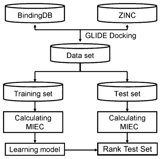
Workflow of MIEC-SVM.
Figure 2.

Building MIEC-SVM model. (1) Generate the complex structure for each ligand in the library using Glide. (2) Calculate MIECs to characterize the protein–ligand interaction. The MIECs are calculated for each protein residue including van der Waals, electrostatic, hydrogen bond, solvation energy (estimated by loss of hydrophobic and hydrophilic surface areas), and geometric constraint (distance between the nearest heavy atoms for each residue–ligand pair). The ligand is represented by a purple ball, and the protease residues are shown as red balls. (3) Assemble the fully filled MIEC matrix, where the response variable y is binary to represent whether the ligand is a binder or nonbinder to the protease and {x1…xN} represent the MIECs for each ligand. (4) Train a support vector machine to analyze the MIEC matrix and build classification models.
We first evaluated the performance of four commonly used kernel functions (linear, polynomial, RBF, and sigmoid) in SVM using the data set with a positive to negative ratio of 1:100. The performance of every kernel function with different K+, which is the weight of the positive samples, was systematically assessed in the range between 0.1 and 20. For every combination of the kernel function and K+, we ran 500 cross validations and calculated the average MCC, Q+, and Q−. We found that linear kernel achieved the best classification accuracy (as indicated by the highest MCC) than any other kernel at any given K+ (Supporting Information Figure S1). Therefore, we used the linear kernel function in all of the following analyses.
In virtual screening, the library contains millions of compounds but only a very small fraction of these compounds bind to a specific target and compounds ranked top in the docking results may have only <1% true positives. Therefore, the positive and negative samples are quite unbalanced. To mimic this scenario, we tested our method on two data sets with different positive to negative ratios R: R = 1:100 and R = 1:200. We used cross validation to evaluate the strategy, which is to train the model with a group of randomly selected samples and assess the model with its performance on another group of samples, which are dissimilar to the training group. To avoid arbitrariness of a single cross validation, we conducted 500 of these cross validations and in each run, we randomly selected 500 positive and 50 000 or 100 000 negative samples. To handle the unbalanced positive and negative samples in SVM, we tested the weight for the positive samples (K+) from 0.1 to 20 and selected the points of MCC reaching plateau as the optimal values: 0.8 for R = 1:100 and 2.6 for R = 1:200.
Using the K+ values determined in each scenario and linear kernel, we observed satisfactory performance of MIEC-SVM on identifying inhibitors of the HIV protease (Table 1). We first trained our model on 1000 positives and 100 000 negatives that were randomly selected from the 1795 positives and 632 033 negatives. Since in virtual screening, the top 5000 to 10 000 compounds are often selected for further evaluation, we limited the size of testing data to 50 positives and 5000 negatives that were randomly selected from the remaining data set. Note that we clustered the positive inhibitors based on their similarity of chemical structures and the testing positives were selected from different clusters of positive compounds in the training set to ensure distinction between training and testing samples. The average MCC of 500 runs of such cross validations was 0.761 and the average AUC was 0.998. Considering how challenging it is to identify the 1% positives, such a performance of our model is satisfactory.
Table 1.
Model Performance in Different Scenarios Assessed by 500 Runs of Cross Validations
| positive to negative ratio | positive to negative ratio | |
|---|---|---|
| R = 1:100 | R = 1:200 | |
| training set | NPos = 1000, NNeg = 100000a | NPos = 1000, NNeg = 200000 |
| test set | NPos = 50, NNeg = 5000 | NPos = 50, NNeg = 10000 |
| Q+ | 0.775 ± 0.057 | 0.626 ± 0.053 |
| Q− | 0.999 ± 0.000 | 0.999 ± 0.000 |
| SE | 0.765 ± 0.166 | 0.840 ± 0.096 |
| SP | 0.999 ± 0.009 | 0.999 ± 0.000 |
| MCC | 0.761 ± 0.116 | 0.722 ± 0.062 |
| AUC | 0.998 ± 0.002 | 0.998 ± 0.002 |
| positives in the top 20 | 15.576 ± 1.923 | 12.990 ± 2.563 |
NPos and NNeg are, respectively, the numbers of positives and negatives in the training or test set.
We next increased the negative to positive ratio to 200. The training/test sets were composed of 1000/50 positives and 200 000/10 000 negatives. The performance was still satisfactory with an average MCC of 0.722 and AUC of 0.998 in 500 independent cross validation runs. Because follow-up experiments are normally only performed on the top ranked compounds from docking, it is important to evaluate the true positive rate Q+. We found that MIEC-SVM could achieve Q+ values of 0.775 and 0.626, respectively, in the two scenarios. In particular, the top 20 ranked compounds in the two scenarios contained on average 15.576 and 12.990 true positives in the 500 test runs. For 499/500 test data sets in the scenario of R = 1:100 and 449/500 test data sets in the scenario of R = 1:200, more than half of the top 20 ligands were true positives (Figure 3).
Figure 3.

Distribution of true positives in the top 20 ligands in the 500 cross-validations. (a) The challenging scenario 1 with a positive/negative ratio R = 1:100. The difference between the MIEC-SVM and either X-score or Glide is statistically significant (both p-value <2.2 × 10⁻¹⁶). (b) The challenging scenario 2 with a positive/negative ratio R = 1:200. The difference between the MIEC-SVM and either X-score or Glide is statistically significant (both p-value <2.2 × 10⁻¹⁶).
Comparison with Other Scoring Functions
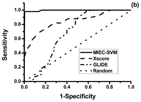
To illustrate the superior performance of our model, we conducted comparison with the docking scores of Glide8–10 and X-score.46 The performance of each score function was evaluated using the area under the ROC curves (AUC) and the number of true positives in the top 20 ligands in the test data sets. Figure 4 shows the ROC curves for the three methods obtained from the same data set in the two scenarios. The average AUC of 500 test data sets in scenario 1 (R = 1:100) is 0.569 for Glide, 0.884 for X-score, and 0.998 for our method. In scenario 2 (R = 1:200), the average AUC is 0.570 for Glide, 0.892 for X-score, and 0.998 for MIEC-SVM. As only a small number of ligands are subject to further evaluation and refinement in drug design, it is important to get as many true positives as possible in the top ranked ligands. Figure 3 shows the distribution of the true positives in the 500 cross validations in the top 20 ligands ranked by the three methods. The average true positives were 9.8, 9.3, and 15.6 for Glide, X-score and MIEC-SVM in scenario 1 and 9.6 for Glide, 6.8 for X-score, and 13.0 for MIEC-SVM in scenario 2. It is very clear that our method outperformed the two state-of-the-art scoring functions assessed by AUC or true positives in the top ranked ligands. One possible reason of the outperformance is that the evaluation is based on the rigid-body docking structures, which may deviate from the real complex structures. In contrary to Glide and X-score that are trained on the crystal structures, our model employs machine learning method (SVM) to reduce its sensitivity to the inaccuracy of the docking structures. On the other hand, such an observation is not completely surprising as both Glide and X-score are general energy functions for all systems but are not specifically designed to rank the HIV protease inhibitors.13 As we have shown in our previous studies, the MIEC-based methods are general and can be applied to diverse systems including domain–peptide interactions27,29–32 and protein–ligand interactions.28 The machine learning method is transferable, but the model needs retraining for a specific system.
Figure 4.

Comparison between MIEC-SVM, Glide, and Xscore on the same data sets using 500 cross validations. The sensitivity and specificity are averaged from the 500 cross validations. (a) The challenging scenario 1 with a positive/negative ratio R = 1:100. (b) The challenging scenario 2 with a positive/negative ratio R = 1:200.
MIEC-SVM Trained with Small Data Sets
In reality, the number of known inhibitors to a drug target, particularly a novel one, is often small. A natural question is whether the MIEC-SVM model can work on other drug targets with a much smaller training set, which is obviously very challenging because small training sets may lead to overfitting. As noted above, it is important to have a high true positive rate in the top ranked compounds because they are the candidates for the follow-up experiments.
In order to detect the minimum size of training set, we systematically shrunk the training set and evaluated the performance of the trained models on the same group of test data sets. First, we randomly generated 500 groups of test data sets for both scenarios of R = 1:100 and R = 1:200. The test data set for the two scenarios respectively contained 50 and 25 positive samples randomly selected from one cluster in the positive data set and 5000 negative samples randomly selected from the negative data set. Second, for each group of test data set, we generated four groups of training data set that respectively contain 500/300/100/50 positive samples. Each training set also respectively contains 50 000/30 000/10 000/5000 negative samples for the scenario R = 1:100 and 100 000/60 000/20 000/10 000 negative samples for the scenario R = 1:200. To keep the diversity between the training data and the test data, all the positive samples in the training set came from ligand clusters different from those in the test set. Finally, we calculated the standard statistics to evaluate the performance of the models (Table 2).
Table 2.
Performance of MIEC-SVM on the Shrunk Training Data Sets R = (a) 1:100 and (b) 1:200
| (a) positive to negative ratio R = 1:100
| ||||
| training set | NPos = 500, NNeg = 50000a | NPos = 300, NNeg = 30000 | NPos = 100, NNeg = 10000 | NPos = 50, NNeg = 5000 |
| test set | NPos = 50, NNeg = 5000 | NPos = 50, NNeg = 5000 | NPos = 50, NNeg = 5000 | NPos = 50, NNeg = 5000 |
| Q+ | 0.783 ± 0.054 (0.811 ± 0.014)b | 0.783 ± 0.058 (0.820 ± 0.017) | 0.776 ± 0.063 (0.863 ± 0.028) | 0.768 ± 0.073 (0.908 ± 0.041) |
| Q− | 0.999 ± 0.000 (0.999 ± 0.000) | 0.999 ± 0.000 (0.999 ± 0.000) | 0.999 ± 0.000 (0.999 ± 0.000) | 0.999 ± 0.000 (0.999 ± 0.000) |
| SE | 0.775 ± 0.080 (0.859 ± 0.021) | 0.736 ± 0.091 (0.836 ± 0.027) | 0.622 ± 0.111 (0.780 ± 0.056) | 0.539 ± 0.128 (0.750 ± 0.082) |
| SP | 0.999 ± 0.000 (0.999 ± 0.000) | 0.999 ± 0.000 (0.999 ± 0.000) | 0.999 ± 0.000 (0.999 ± 0.000) | 0.999 ± 0.000 (0.999 ± 0.000) |
| MCC | 0.776 ± 0.055 (0.833 ± 0.015) | 0.756 ± 0.063 (0.826 ± 0.019) | 0.690 ± 0.078 (0.819 ± 0.036) | 0.637 ± 0.096 (0.822 ± 0.053) |
| AUC | 0.998 ± 0.002 | 0.995 ± 0.007 | 0.992 ± 0.014 | 0.987 ± 0.019 |
| positives in the top 20 | 15.882 ± 1.814 | 15.848 ± 1.861 | 15.724 ± 1.958 | 15.686 ± 1.979 |
|
| ||||
| (b) positive to negative ratio R = 1:200 | ||||
|
| ||||
| training set | NPos = 500, NNeg = 100000a | NPos = 300, NNeg = 60000a | NPos = 100, NNeg = 20000a | NPos = 50, NNeg = 10000a |
| test set | NPos = 25, NNeg = 5000 | NPos = 25, NNeg = 5000 | NPos = 25, NNeg = 5000 | NPos = 25, NNeg = 5000 |
| Q+ | 0.643 ± 0.070 (0.657 ± 0.013)b | 0.638 ± 0.070 (0.667 ± 0.017) | 0.632 ± 0.077 (0.703 ± 0.031) | 0.624 ± 0.082 (0.748 ± 0.046) |
| Q− | 0.999 ± 0.000 (0.999 ± 0.000) | 0.999 ± 0.000 (0.999 ± 0.000) | 0.999 ± 0.000 (0.999 ± 0.000) | 0.999 ± 0.000 (0.999 ± 0.000) |
| SE | 0.891 ± 0.070 (0.947 ± 0.010) | 0.856 ± 0.084 (0.941 ± 0.013) | 0.765 ± 0.112 (0.928 ± 0.025) | 0.682 ± 0.122 (0.925 ± 0.039) |
| SP | 0.999 ± 0.000 (0.999 ± 0.000) | 0.999 ± 0.000 (0.999 ± 0.000) | 0.999 ± 0.000 (0.999 ± 0.000) | 0.999 ± 0.000(0.999 ± 0.000) |
| MCC | 0.754 ± 0.058 (0.787 ± 0.010) | 0.736 ± 0.062 (0.790 ± 0.013) | 0.692 ± 0.079 (0.806 ± 0.024) | 0.648 ± 0.086 (0.831 ± 0.036) |
| AUC | 0.997 ± 0.004 | 0.997 ± 0.003 | 0.995 ± 0.009 | 0.990 ± 0.018 |
| positives in the top 20 | 12.728 ± 2.078 | 12.66 ± 1.955 | 12.066 ± 2.003 | 11.860 ± 1.991 |
NPos and NNeg are respectively the numbers of positives and negatives in the training or test set.
The numbers in the parentheses are the values for the training data sets in the 500 cross-validation runs.
In both scenarios, we observed that the models trained from 500 and 300 positive samples showed no overfitting as indicated by comparable performance of the models in the training and test sets. When smaller training sets were used, overfitting started to emerge. The models trained on 100 positives and 10 000 or 20 000 negatives showed larger drop of performance in the test set from the training set and such a drop became more significant for the models trained on 50 positive and 5000/10 000 negative samples (the decrease of MCC was about 0.2). Interestingly, the models trained on smaller number of positives (100 or 50 samples) still showed high accuracy, and AUC (Q+ equals to 0.624, AUC = 0.990 for the most difficult case that the model was trained on 50 positives samples with R = 1:200), as well as the enrichment of true positives in the top 20 ligands (11.86 for the most difficult case). Taken together, these observations suggest that the MIEC-SVM models are able to find new inhibitors for a target protein that has 50 known inhibitors.
For many important drug targets, it is not uncommon to have 50 known inhibitors, but new inhibitors are still in urgent need to reduce toxicity or improve efficacy. We thus further investigated whether our method trained on 50 positive samples can still find new inhibitors. As the 50 available inhibitors for a target can have diverse chemical structures, we took the following “model average” strategy to exploit the diversity presented in the training set. We randomly selected 40 positive and 4000 negative samples to train 500 models. Each of these models was used to score compounds in the library. A compound was predicted as an inhibitor if a certain number of models classify it as positive. In this study, we chose a cutoff of 1, i.e. at least one model predicted the compound as a positive. To examine the effectiveness of this strategy and how the training data influences the performance, we constructed 500 test data sets of 50 positive and 5000 negative samples, in which the 50 positive samples were randomly selected from five clusters, 10 from each cluster. The training data sets contained another 50 positive and 5000 negative samples, while positive samples were selected from same or different clusters (Table 3). We constructed 31 training data sets that exhaustively selected samples from all possible combinations of the five positive clusters. We observed that our models predicted less than 60 inhibitors and among which around 70% were true positives. Considering that true positives account for only 1% of the test set, such a performance is satisfactory, which also suggests the robustness of the MIEV-SVM method.
Table 3.
Performance of MIEC-SVM Trained on 50 Positive and 5000 Negative Samples
| clusters in the traininga | TP | FP | TN | FN | Q+ |
|---|---|---|---|---|---|
| 1 | 41.35 ± 3.32 | 17.73 ± 4.39 | 4982.27 ± 4.39 | 8.65 ± 3.32 | 0.70 ± 0.05 |
| 2 | 41.31 ± 2.99 | 18.70 ± 4.47 | 4981.30 ± 4.47 | 8.69 ± 2.99 | 0.69 ± 0.05 |
| 3 | 42.10 ± 3.05 | 19.63 ± 4.96 | 4980.37 ± 4.96 | 7.90 ± 3.05 | 0.69 ± 0.06 |
| 4 | 39.34 ± 3.77 | 18.02 ± 4.62 | 4981.98 ± 4.62 | 10.66 ± 3.77 | 0.69 ± 0.06 |
| 5 | 41.79 ± 3.06 | 18.54 ± 4.39 | 4981.46 ± 4.39 | 8.21 ± 3.06 | 0.70 ± 0.05 |
| 1,2 | 42.97 ± 2.77 | 18.62 ± 4.71 | 4981.38 ± 4.71 | 7.03 ± 2.77 | 0.70 ± 0.05 |
| 1,3 | 43.05 ± 2.91 | 19.04 ± 4.88 | 4980.96 ± 4.88 | 6.95 ± 2.91 | 0.70 ± 0.06 |
| 1,4 | 42.42 ± 3.16 | 17.80 ± 4.62 | 4982.20 ± 4.62 | 7.58 ± 3.16 | 0.71 ± 0.05 |
| 1,5 | 42.82 ± 3.09 | 18.54 ± 4.75 | 4981.46 ± 4.75 | 7.18 ± 3.09 | 0.70 ± 0.05 |
| 2,3 | 42.17 ± 3.08 | 19.19 ± 4.53 | 4980.81 ± 4.53 | 7.83 ± 3.08 | 0.69 ± 0.05 |
| 2,4 | 41.07 ± 3.26 | 18.28 ± 4.62 | 4981.72 ± 4.62 | 8.93 ± 3.26 | 0.70 ± 0.05 |
| 2,5 | 42.30 ± 2.99 | 18.86 ± 4.61 | 4981.14 ± 4.61 | 7.70 ± 2.99 | 0.69 ± 0.05 |
| 3,4 | 42.40 ± 3.02 | 19.01 ± 4.70 | 4980.99 ± 4.70 | 7.60 ± 3.02 | 0.69 ± 0.05 |
| 3,5 | 42.08 ± 2.83 | 19.30 ± 4.60 | 4980.70 ± 4.60 | 7.92 ± 2.83 | 0.69 ± 0.05 |
| 4,5 | 41.66 ± 3.28 | 18.36 ± 4.66 | 4981.64 ± 4.66 | 8.34 ± 3.28 | 0.70 ± 0.05 |
| 1,2,3 | 42.99 ± 2.89 | 19.27 ± 4.54 | 4980.73 ± 4.54 | 7.01 ± 2.89 | 0.69 ± 0.05 |
| 1,2,4 | 42.60 ± 3.02 | 18.40 ± 4.64 | 4981.60 ± 4.64 | 7.40 ± 3.02 | 0.70 ± 0.05 |
| 1,2,5 | 43.11 ± 2.79 | 19.06 ± 4.82 | 4980.94 ± 4.82 | 6.89 ± 2.79 | 0.70 ± 0.05 |
| 1,3,4 | 43.04 ± 2.93 | 18.80 ± 4.85 | 4981.20 ± 4.85 | 6.96 ± 2.93 | 0.70 ± 0.06 |
| 1,3,5 | 42.95 ± 2.82 | 19.15 ± 4.66 | 4980.85 ± 4.66 | 7.05 ± 2.82 | 0.70 ± 0.05 |
| 1,4,5 | 42.72 ± 3.07 | 18.44 ± 4.62 | 4981.56 ± 4.62 | 7.28 ± 3.07 | 0.70 ± 0.05 |
| 2,3,4 | 42.16 ± 3.06 | 18.96 ± 4.94 | 4981.04 ± 4.94 | 7.84 ± 3.06 | 0.69 ± 0.06 |
| 2,3,5 | 42.20 ± 2.89 | 19.05 ± 4.63 | 4980.95 ± 4.63 | 7.80 ± 2.89 | 0.69 ± 0.05 |
| 2,4,5 | 42.11 ± 3.16 | 18.75 ± 4.88 | 4981.25 ± 4.88 | 7.89 ± 3.16 | 0.70 ± 0.06 |
| 3,4,5 | 42.41 ± 3.06 | 18.91 ± 4.78 | 4981.09 ± 4.78 | 7.59 ± 3.06 | 0.70 ± 0.05 |
| 1,2,3,4 | 43.04 ± 3.04 | 19.00 ± 4.65 | 4981.00 ± 4.65 | 6.96 ± 3.04 | 0.70 ± 0.05 |
| 1,2,3,5 | 42.68 ± 2.80 | 19.02 ± 4.70 | 4980.98 ± 4.70 | 7.32 ± 2.80 | 0.70 ± 0.05 |
| 1,2,4,5 | 42.62 ± 2.94 | 18.65 ± 4.84 | 4981.35 ± 4.84 | 7.38 ± 2.94 | 0.70 ± 0.05 |
| 1,3,4,5 | 43.06 ± 2.81 | 18.84 ± 4.71 | 4981.16 ± 4.71 | 6.94 ± 2.81 | 0.70 ± 0.05 |
| 2,3,4,5 | 42.26 ± 2.95 | 19.19 ± 5.01 | 4980.81 ± 5.01 | 7.74 ± 2.95 | 0.69 ± 0.06 |
| 1,2,3,4,5 | 42.89 ± 2.95 | 18.99 ± 4.74 | 4981.01 ± 4.74 | 7.11 ± 2.95 | 0.70 ± 0.05 |
| average | 42.27 ± 3.14 | 18.76 ± 4.71 | 4981.23 ± 4.71 | 7.72 ± 3.14 | 0.70 ± 0.05 |
Clusters from which the training samples were selected.
Most Informative MIECs and Protease Residues for Protease–Ligand Binding
Encouraged by the success of the MIEC-SVM model on scoring the docking poses, we next conducted feature selection to search for the most informative MIECs and protein residues for protein–ligand binding. Given the large number of possible combinations of six MIECs and 99 protease residues, we took a two-step heuristic strategy in which we found the informative MIECs in the first step and then the informative residues in the second step.
In the first step, we trained and tested the models with different MIEC terms in scenario 1 with a positive/negative ratio R = 1:100 (Table 4). Using any single MIEC, the model showed a significant drop of sensitivity and a smaller decrease of MCC except the hydrogen-bond term, which may be due to the difficulty of correctly reconstructing hydrogen bonds in docking. The polar hydrogen atoms are rotatable and such rotation is often not considered by the docking program. In addition, the hydrogen bond energy is calculated based on the distance between the hydrogen atom and the acceptor atom, as well as the angle formed between the hydrogen donor and acceptor atoms, all of which are sensitive to the position of the hydrogen atom.
Table 4.
Prediction Performance of Different Combinations of Descriptors
| MIECs | Q+ | SE | MCC |
|---|---|---|---|
| alla | 0.775b ± 0.057 | 0.765 ± 0.109 | 0.761 ± 0.116 |
| ΔEvdw | 0.783 ± 0.074 | 0.482 ± 0.095 | 0.609 ± 0.080 |
| ΔEelec | 0.731 ± 0.101 | 0.457 ± 0.131 | 0.571 ± 0.116 |
| ΔEhbond | 0.719 ± 0.123 | 0.192 ± 0.064 | 0.366 ± 0.084 |
| Dnear | 0.770 ± 0.068 | 0.523 ± 0.079 | 0.630 ± 0.065 |
| ΔAphobic | 0.775 ± 0.076 | 0.504 ± 0.099 | 0.620 ± 0.083 |
| ΔAphilic | 0.770 ± 0.059 | 0.656 ± 0.081 | 0.707 ± 0.060 |
| ΔEvdw, Dnear | 0.770 ± 0.059 | 0.729 ± 0.093 | 0.746 ± 0.066 |
| ΔEvdw, ΔAphilic | 0.771 ± 0.056 | 0.756 ± 0.098 | 0.760 ± 0.067 |
| ΔEelec, Dnear | 0.769 ± 0.059 | 0.721 ± 0.098 | 0.741 ± 0.068 |
| ΔEelec, ΔAphilic | 0.775 ± 0.057 | 0.747 ± 0.095 | 0.757 ± 0.066 |
| ΔEhbond, Dnear | 0.771 ± 0.061 | 0.595 ± 0.076 | 0.673 ± 0.060 |
| ΔEhbond, ΔAphilic | 0.774 ± 0.056 | 0.686 ± 0.074 | 0.725 ± 0.055 |
| Dnear, ΔAphobic | 0.786 ± 0.054 | 0.750 ± 0.072 | 0.765 ± 0.052 |
| Dnear, ΔAphilic | 0.778 ± 0.054 | 0.772 ± 0.088 | 0.771 ± 0.060 |
| ΔAphobic, ΔAphilic | 0.775 ± 0.060 | 0.676 ± 0.080 | 0.720 ± 0.060 |
| ΔEvdw, Dnear, ΔAphobic | 0.783 ± 0.054 | 0.794 ± 0.085 | 0.785 ± 0.057 |
| ΔEvdw, Dnear, ΔAphilic | 0.773 ± 0.055 | 0.789 ± 0.100 | 0.777 ± 0.066 |
| ΔEelec, Dnear, ΔAphobic | 0.780 ± 0.054 | 0.776 ± 0.088 | 0.775 ± 0.061 |
| ΔEelec, Dnear, ΔAphilic | 0.775 ± 0.055 | 0.789 ± 0.101 | 0.779 ± 0.068 |
| ΔEhbond, Dnear, ΔAphobic | 0.784 ± 0.053 | 0.748 ± 0.073 | 0.762 ± 0.051 |
| ΔEhbond, Dnear, ΔAphilic | 0.778 ± 0.053 | 0.775 ± 0.080 | 0.774 ± 0.055 |
| Dnear, ΔAphobic, ΔAphilic | 0.782 ± 0.054 | 0.776 ± 0.080 | 0.776 ± 0.056 |
| ΔEvdw,ΔEelec, Dnear, ΔAphobic | 0.779 ± 0.055 | 0.787 ± 0.093 | 0.779 ± 0.057 |
| ΔEvdw, ΔEelec, Dnear, ΔAphilic | 0.771 ± 0.055 | 0.781 ± 0.078 | 0.772 ± 0.060 |
| ΔEvdw, ΔEhbond, Dnear, ΔAphobic | 0.779 ± 0.054 | 0.773 ± 0.088 | 0.773 ± 0.062 |
| ΔEvdw, Dnear, ΔAphobic, ΔAphilic | 0.778 ± 0.055 | 0.784 ± 0.077 | 0.778 ± 0.052 |
| ΔEelec, ΔEhbond, Dnear, ΔAphilic | 0.775 ± 0.053 | 0.777 ± 0.063 | 0.772 ± 0.058 |
| ΔEelec, Dnear, ΔAphobic, ΔAphilic | 0.780 ± 0.053 | 0.778 ± 0.081 | 0.776 ± 0.053 |
| ΔEvdw, ΔEelec, Dnear, ΔAphobic, ΔAphilic | 0.776 ± 0.056 | 0.772 ± 0.076 | 0.770 ± 0.055 |
| ΔEvdw, ΔEhbond, Dnear, ΔAphobic, ΔAphilic | 0.778 ± 0.062 | 0.766 ± 0.083 | 0.768 ± 0.052 |
| Dnear, ΔEvdw, ΔEelec, ΔEhbond, ΔAphobic | 0.777 ± 0.031 | 0.767 ± 0.072 | 0.768 ± 0.042 |
ΔEvdw, van der Waals energy; ΔEelec, electrostatic energy; ΔEhbond, hydrogen bond energy; Dnear, geometry constraint measured by the nearest distance between heavy atoms of the protein residue and the ligand; ΔAphobic, loss of hydrophobic SASA upon binding; ΔAphilic, loss of hydrophilic area upon binding. bThe average values calculated from 500 cross validations.
We next examined the performances of different MIEC combinations using a greedy algorithm. We started with the two MIECs with the best MCCs, ΔAphilic, and Dnear, as the seed. The combinations of the seeds with all other MIECs were tested. Then the two best performed combinations were kept as the seeds for the next iteration until the number of included MIECs reached five (Table 4). For example, the two best performed 3-MIEC models were trained on ΔEvdw, Dnear, ΔAphobic and ΔEvdw, Dnear, ΔAphilic, which were selected as seeds for the next iteration to find the best performed 4-MIEC models. Using this greedy search strategy, we found that the model trained on ΔEvdw, Dnear, and ΔAphobic performed best, even better than using all MIECs. This finding is not totally unexpected as these MIECs are less sensitive to the conformational flexibility and inaccuracy in docking than the other terms: ΔEvdw characterizes the short-range interactions of the binding, Dnear represents the geometry constraint and shape complementarity, and ΔAphobic estimates the solvation energy based on the loss of hydrophobic SASA. Interestingly, the second-best performing 3-MIEC model is ΔEele, Dnear, and ΔAphilic. Both ΔAphilic and ΔAphobic estimate the ation energy, but they are respectively complementary to ΔEele and ΔEvdw. Therefore, it is not surprising that these two combinations showed similar performance.
We next searched for residues important for recognition using the best performed combination of Dnear, ΔAphobic, and ΔEvdw. We first evaluated the contribution of each position by examining the change of MCC when leaving it out in the model, i.e. all the MIECs with which this position is associated were removed from the model (leave-one-position-out test). The positions with the largest MCC drop were used as the seed for a greedy search to find the most critical combinations of two positions. This procedure was repeated until no position was left for consideration. Figure 5 shows the best performed combination of 38 positions with an average MCC of 0.802 in 500 cross validations for the scenario 1 (R = 1:100), as compared with MCC of 0.785 using all the positions. We also tested this model in scenario 2 (R = 1:100), and the average MCC was 0.762, improved from 0.734 using all the positions. Most of the 38 residues are around the binding pocket (Figure 6), including the catalytic dyad and their neighbor residues (residue 23–27). Interestingly, the 38 positions also include several residues at which drug resistant mutations often occur, such as positions 10, 48, 54, and 90. We speculate that reducing an inhibitor’s interaction with these residues may improve its potency to combat resistance.
Figure 5.

Selecting the most informative positions in the MIEC-SVM model using the best combination of three MIECs of Dnear, ΔAphobic, and ΔEvdw. The MCC is given by the best performed group of residues in the “leave-one-residue-out” test and is the average of 500 cross validations in the challenging scenario 1 with a positive to negative ratio R = 1:100. The best performing positions are shown in Supporting Information Table S2.
Figure 6.
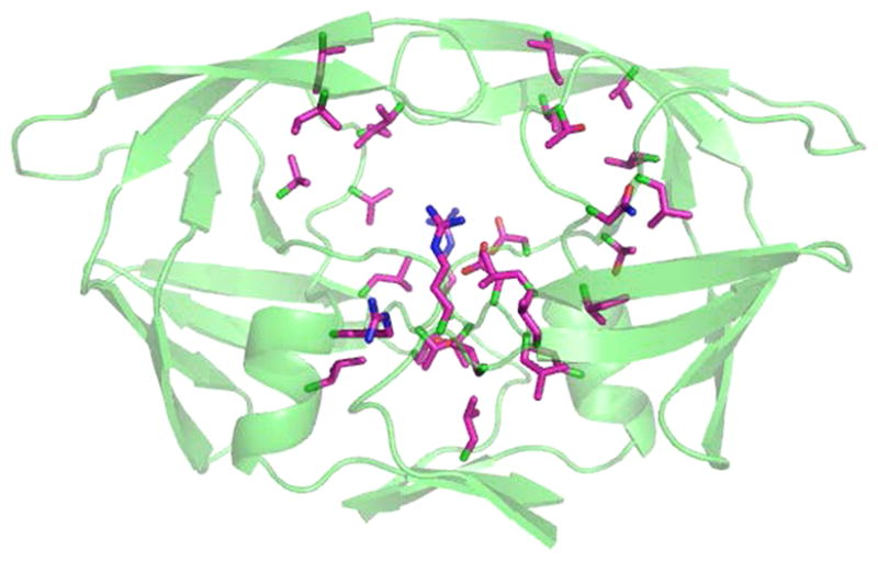
Selected positions from feature selection in the HIV-protease structure. The selected positions are shown in purple. Most of the residues are around the binding pockets. The positions that are far from the pockets are often the hot-spots of drug-resistant mutants, such as 10, 90, 48, and 54.
CONCLUSION
Previously, we have demonstrated the effectiveness of MIEC-SVM in capturing the binding modes of protein–peptide and protein–ligand interactions.27–32 In this study, we further generalized this model and applied to a more challenging problem of identifying strong inhibitors in virtual screening in which the complex structures were generated from docking programs that may be inaccurate and noisy. In spite of these challenges, the MIEC-SVM model showed satisfactory performance on ranking the inhibitors in the difficult scenarios with very small positive to negative ratio (1:100 and 1:200). Measured by AUC as well as the true positives in the top 20 ligands, MIEC-SVM performed significantly better than the state-of-the-art scoring functions such as Glide and X-score. As the HIV protease is the primary drug target for the AIDS therapy and drug resistance was observed for all the drugs, this scoring function specifically designed for the HIV-1 protease would be useful in searching for and designing new inhibitors that are distinct from the currently available drugs and help to develop new therapeutic treatments for AIDS.
An especially encouraging observation is that the MIEC-SVM model showed significant enrichment of true positives in the top 20 candidates, even trained on a data set as small as 50 known inhibitors. In particular, we found that model average can further improve the enrichment using training set containing small number of positives. Such a robustness of MIEC-SVM suggests that the model captures the energetic and geometric characteristics of the protein–ligand binding. This feature is particularly important for finding new inhibitors for novel drug targets because the number of known inhibitors against these targets is often small. In addition, MIEC-SVM consistently outperformed the state-of-the-art scoring functions of Glide and X-score in the scenario where a small percentage (1% or 0.5%) of a small number of positives is present in the compound library. Taken together, we believe that the MIEC-SVM method is a powerful tool for finding strong inhibitors in virtual screening.
EXPERIMENTAL SECTION
Data Set
Figure 1 shows the work flow of the model building and model evaluation process. The ligand data set for training and testing the models were assembled from the BindingDB33 and ZINC34 database. From BindingDB, we retrieved 4486 unique ligands with known binding affinity to the HIV-1 protease, and their dissociation constants (Kd) range from 10−1 to 10−14 M. These ligands were classified into 2072 positive and 2405 negative samples using an artificial cutoff of 10 nM. Nine samples with conflicting binding affinities measured by different experiments were discarded.
All the ligands were docked to an HIV-1 protease template structure (PDB code: 1HPV35) using Glide.8,9 As indicated by a favorable (negative) energy (Coulomb plus van der Waals) calculated by Glide, 1795 positive and 2038 negative complexes were docked successfully. Obviously, the portion of positives (47%) is much larger than that commonly seen in virtual screening (~1%). To mimic the reality, we increased the number of negatives by selecting ~647 000 compounds from the ZINC database34 that passed the Lipinski’s drug-like filters.36 All these compounds were docked into the protease template structure with consideration of all enantiomers. To avoid including any true inhibitor from these drug-like compounds, we removed the top 20 000 conformations ranked by Glide and added the remaining 629 995 conformations to the negative set. As a result, there were 1795 positive and 632 033 negative samples.
Protein Preparation and Docking Procedure
The HIV-1 protease template structure (PDB code: 1HPV35) was subject to multiple preparation steps as suggested in Maestro’s protein preparation wizard in Glide. First, water molecules were removed, bond orders were assigned, and hydrogen atoms were added. Second, protonation and tautomeric state of His, orientation of amide in Asn and Gln, hydroxyl in Ser, Thr, and Tyr, and thiol groups in Cys were optimized sequentially by hydrogen position optimization and exhaustive sampling options. The preparation step was finished by restrained minimization of ligand/protein complexes using OPLS_2001 force field.37,38
Docking was performed by Glide,8,9 which utilized precomputed grids. The grids were generated using the centroid of the ligand in the template structure as the origin. The grid box size for the centroid of the docking ligands was 10 Å × 10 Å × 10 Å, while the size for all the atoms in the ligands was 30 Å × 30 Å × 30 Å. All the complex models of candidate ligands were constructed with Glide-SP (standard-precision) docking with van der Waals radius scaling of 0.8 and a partial charge cutoff of 0.25. The options of ring conformation sampling and nitrogen inversion were turned on in the docking as well. For each ligand, up to 10 top scored conformations were saved for later data analysis.
Calculation of MIECs
To characterize the binding, we identified all 64 protease residues located within 12 Å of the grid center in the complex structures generated by Glide (Figure 2). For each residue, we calculated the following MIECs: van der Waals (ΔEvdw), electrostatic (ΔEelec), hydrogen bond (ΔEH-bond), desolvation energy, and geometry constraint (Dnear, which is the distance of the nearest heavy atom-pair between the residue and ligand). ΔEvdw, ΔEelec, ΔEH-bond, and Dnear were taken from the output of Glide. The solvation energy was estimated by the solvent accessible surface area (SASA).39 SASA for each atom was calculated using the method developed by Street and Mayo.40 The radii of the atoms for the SASA calculation were taken from AMBER0341 and general AMBER force field (gaff),42 and the probe radius was set to 1.4 Å. The atoms were also classified into hydrophobic and hydrophilic types based on the functional groups they belong to (Supporting Information Table S1). The loss of hydrophobic and hydrophilic surface areas (ΔAphobic and ΔAphilic) upon binding were calculated separately to discriminate their opposite contributions to binding. As shown in Figure 2, the interaction between the protein and the ligand was described using a vector, which contains the different types of interactions between each residue and the ligand.
Training and Testing the Model
In order to rigorously assess whether our method can identify inhibitors dissimilar to the ones in the training set, we first clustered the positives using an average linkage clustering method,43 in which the similarity of two clusters was measured by the average pairwise similarity of the ligands in these two clusters, using a metric of ligand similarity calculated by Openbabel with the Tanimoto method.44 Forty-five clusters were found using a cutoff of 0.5, and the size of the clusters ranges from 1 to 350. The clusters were consolidated into five groups with the same size so that every sample has the same chance to be selected for training or testing. For a cross validation, the positive samples in the training set were randomly selected from four clusters and those in the test set were randomly selected from the remaining cluster to ensure that similar compounds were not included in both training and test sets. The negative samples in the training and test sets were randomly selected, as they were taken from the ZINC database34 and are unlikely analogs.
We used cross validation to evaluate our method with 1000 positive samples in the training set and 50 positive samples in the test set. We mimicked different scenarios by mixing the positive samples with different number of negative samples. Because the clusters were generated using average linkage hierarchical clustering, it is still possible that a small number of positive samples in the test set have a similarity greater than 0.5 with ligands in the training set. We observed comparable performances of our models when keeping and removing the ligands with >0.5 similarity scores in the test set (MCC = 0.984 ± 0.023 and 0.980 ± 0.054, respectively, on 500 cross validations), which indicated the robustness of our method.
Training Support Vector Machine
Each column of the MIEC matrix in Figure 2 was normalized by the maximum value. A support vector machine (SVM) was then trained to classify compounds as inhibitors and noninhibitors of the HIV protease. The LIBSVM45 program was employed in this study. The performance of the models was evaluated by 500 runs of cross validations. TP (true positives), FP (false positives), TN (true negatives), and FN (false negatives) obtained in the 500 test sets were counted separately. The following standard statistics were then computed: prediction accuracy of positive samples Q+ = TP/(TP + FP); prediction accuracy of negative samples Q– = TN/(TN + FN); sensitivity SE = TP/(TP + FN); specificity SP = TN/(TN + FP); and Matthews correlation coefficient MCC = (TP × TN – FP × FN)/((TP + FP)(TP + FN)(TN + FN)(TN + FP))1/2. We also plotted the receiver operating characteristic (ROC) curve and calculated the AUC (area under the curve). The ROC curve was obtained from the real values calculated by SVM to judge whether the samples were positive or negative: the larger a value, the more likely a sample is classified as a positive.
Supplementary Material
Acknowledgments
This project was partially supported by the NIH (R01GM-085188 to W.W.).
ABBREVIATIONS
- MIEC
molecular interaction energy component
- SVM
support vector machine
- SASA
solvent accessible surface area
- TP
true positive
- FP
false positive
- TN
true negative
- FN
false negative
- Q+
accuracy of positive samples
- Q–
accuracy of negative samples
- SP
specificity
- SE
sensitivity
- MCC
Matthews correlation coefficient
- ROC
receiver operating characteristic
- AUC
area under the curve
Footnotes
Author Contributions
B.D. and W.W. conceived and designed the study. B.D. performed the experiments and analyzed the results. J.W. contributed to the docking analysis. N.L. contributed to developing the computational models. B.D. and W.W. wrote the manuscript.
Notes
The authors declare no competing financial interest.
The list of hydrophobic and hydrophilic atoms; the list of best performance residues with greedy algorithm; selection of kernel function and weights for positive samples in SVM. This material is available free of charge via the Internet at http://pubs.acs.org.
References
- 1.Knegtel RM, Wagener M. Efficacy and selectivity in flexible database docking. Proteins. 1999;37(3):334–45. doi: 10.1002/(sici)1097-0134(19991115)37:3<334::aid-prot3>3.0.co;2-9. [DOI] [PubMed] [Google Scholar]
- 2.Pauli I, Timmers LFSM, Caceres RA, Soares MBP, de Azevedo WF. In silico and in vitro: identifying new drugs. Curr Drug Targets. 2008;9(12):1054–1061. doi: 10.2174/138945008786949397. [DOI] [PubMed] [Google Scholar]
- 3.Rarey M, Kramer B, Lengauer T, Klebe G. A fast flexible docking method using an incremental construction algorithm. J Mol Biol. 1996;261(3):470–89. doi: 10.1006/jmbi.1996.0477. [DOI] [PubMed] [Google Scholar]
- 4.Rarey M, Kramer B, Lengauer T. The particle concept: placing discrete water molecules during protein-ligand docking predictions. Proteins. 1999;34(1):17–28. [PubMed] [Google Scholar]
- 5.Morris GM, GDS, Halliday RS, Huey R, Hart WE, Belew RK, OAJ Automated Docking Using a Lamarckian Genetic Algorithm and an Empirical Binding Free Energy Function. J Comput Chem. 1998;19:1639–1662. [Google Scholar]
- 6.Morris GM, Goodsell DS, Huey R, Olson AJ. Distributed automated docking of flexible ligands to proteins: parallel applications of AutoDock 2.4. J Comput Aided Mol Des. 1996;10(4):293–304. doi: 10.1007/BF00124499. [DOI] [PubMed] [Google Scholar]
- 7.Goodsell DS, Olson AJ. Automated docking of substrates to proteins by simulated annealing. Proteins. 1990;8(3):195–202. doi: 10.1002/prot.340080302. [DOI] [PubMed] [Google Scholar]
- 8.Halgren TA, Murphy RB, Friesner RA, Beard HS, Frye LL, Pollard WT, Banks JL. Glide: a new approach for rapid, accurate docking and scoring. 2. Enrichment factors in database screening. J Med Chem. 2004;47(7):1750–9. doi: 10.1021/jm030644s. [DOI] [PubMed] [Google Scholar]
- 9.Friesner RA, Banks JL, Murphy RB, Halgren TA, Klicic JJ, Mainz DT, Repasky MP, Knoll EH, Shelley M, Perry JK, Shaw DE, Francis P, Shenkin PS. Glide: a new approach for rapid, accurate docking and scoring. 1. Method and assessment of docking accuracy. J Med Chem. 2004;47(7):1739–49. doi: 10.1021/jm0306430. [DOI] [PubMed] [Google Scholar]
- 10.Friesner RA, Murphy RB, Repasky MP, Frye LL, Greenwood JR, Halgren TA, Sanschagrin PC, Mainz DT. Extra precision glide: docking and scoring incorporating a model of hydrophobic enclosure for protein-ligand complexes. J Med Chem. 2006;49(21):6177–96. doi: 10.1021/jm051256o. [DOI] [PubMed] [Google Scholar]
- 11.Jones G, Willett P, Glen RC, Leach AR, Taylor R. Development and validation of a genetic algorithm for flexible docking. J Mol Biol. 1997;267(3):727–48. doi: 10.1006/jmbi.1996.0897. [DOI] [PubMed] [Google Scholar]
- 12.Jones G, Willett P, Glen RC. Molecular recognition of receptor sites using a genetic algorithm with a description of desolvation. J Mol Biol. 1995;245(1):43–53. doi: 10.1016/s0022-2836(95)80037-9. [DOI] [PubMed] [Google Scholar]
- 13.Kim R, Skolnick J. Assessment of programs for ligand binding affinity prediction. J Comput Chem. 2008;29(8):1316–31. doi: 10.1002/jcc.20893. [DOI] [PMC free article] [PubMed] [Google Scholar]
- 14.Cheng T, Li X, Li Y, Liu Z, Wang R. Comparative assessment of scoring functions on a diverse test set. J Chem Inf Model. 2009;49(4):1079–1093. doi: 10.1021/ci9000053. [DOI] [PubMed] [Google Scholar]
- 15.Altman MD, Ali A, Reddy GSKK, Nalam MNL, Anjum SG, Cao H, Chellappan S, Kairys V, Fernandes MX, Gilson MK, Schiffer CA, Rana TM, Tidor B. HIV-1 protease inhibitors from inverse design in the substrate envelope exhibit subnanomolar binding to drug-resistant variants. J Am Chem Soc. 2008;130(19):6099–6113. doi: 10.1021/ja076558p. [DOI] [PMC free article] [PubMed] [Google Scholar]
- 16.Jorissen RN, Reddy GSKK, Ali A, Altman MD, Chellappan S, Anjum SG, Tidor B, Schiffer CA, Rana TM, Gilson MK. Additivity in the analysis and design of HIV protease inhibitors. J Med Chem. 2009;52(3):737–754. doi: 10.1021/jm8009525. [DOI] [PMC free article] [PubMed] [Google Scholar]
- 17.Nalam MNL, Ali A, Altman MD, Reddy GSKK, Chellappan S, Kairys V, Ozen A, Cao H, Gilson MK, Tidor B, Rana TM, Schiffer CA. Evaluating the substrate-envelope hypothesis: structural analysis of novel HIV-1 protease inhibitors designed to be robust against drug resistance. J Virol. 2010;84(10):5368–5378. doi: 10.1128/JVI.02531-09. [DOI] [PMC free article] [PubMed] [Google Scholar]
- 18.Fabry-Asztalos L, Andonie R, Collar CJ, Abdul-Wahid S, Salim N. A genetic algorithm optimized fuzzy neural network analysis of the affinity of inhibitors for HIV-1 protease. Bioorg Med Chem. 2008;16(6):2903–2911. doi: 10.1016/j.bmc.2007.12.055. [DOI] [PubMed] [Google Scholar]
- 19.Geppert H, Horváth T, Gärtner T, Wrobel S, Bajorath J. Support-vector-machine-based ranking significantly improves the effectiveness of similarity searching using 2D fingerprints and multiple reference compounds. J Chem Inf Model. 2008;48(4):742–746. doi: 10.1021/ci700461s. [DOI] [PubMed] [Google Scholar]
- 20.Agarwal S, Dugar D, Sengupta S. Ranking chemical structures for drug discovery: a new machine learning approach. J Chem Inf Model. 2010;50(5):716–731. doi: 10.1021/ci9003865. [DOI] [PubMed] [Google Scholar]
- 21.Ballester PJ, Mitchell JBO. A machine learning approach to predicting protein-ligand binding affinity with applications to molecular docking. Bioinformatics. 2010;26(9):1169–1175. doi: 10.1093/bioinformatics/btq112. [DOI] [PMC free article] [PubMed] [Google Scholar]
- 22.Marcou G, Rognan D. Optimizing fragment and scaffold docking by use of molecular interaction fingerprints. J Chem Inf Model. 2007;47(1):195–207. doi: 10.1021/ci600342e. [DOI] [PubMed] [Google Scholar]
- 23.Deng Z, Chuaqui C, Singh J. Structural interaction fingerprint (SIFt): a novel method for analyzing three-dimensional protein-ligand binding interactions. J Med Chem. 2004;47(2):337–44. doi: 10.1021/jm030331x. [DOI] [PubMed] [Google Scholar]
- 24.Perez-Nueno VI, Rabal O, Borrell JI, Teixido J. APIF: a new interaction fingerprint based on atom pairs and its application to virtual screening. J Chem Inf Model. 2009;49(5):1245–60. doi: 10.1021/ci900043r. [DOI] [PubMed] [Google Scholar]
- 25.Brewerton SC. The use of protein-ligand interaction fingerprints in docking. Curr Opin Drug Discov Devel. 2008;11(3):356–64. [PubMed] [Google Scholar]
- 26.Sato T, Honma T, Yokoyama S. Combining machine learning and pharmacophore-based interaction fingerprint for in silico screening. J Chem Inf Model. 2010;50(1):170–185. doi: 10.1021/ci900382e. [DOI] [PubMed] [Google Scholar]
- 27.Hou T, Zhang W, Case DA, Wang W. Characterization of domain-peptide interaction interface: a case study on the amphiphysin-1 SH3 domain. J Mol Biol. 2008;376(4):1201–14. doi: 10.1016/j.jmb.2007.12.054. [DOI] [PubMed] [Google Scholar]
- 28.Hou T, Zhang W, Wang J, Wang W. Predicting drug resistance of the HIV-1 protease using molecular interaction energy components. Proteins. 2009;74(4):837–46. doi: 10.1002/prot.22192. [DOI] [PMC free article] [PubMed] [Google Scholar]
- 29.Hou T, Xu Z, Zhang W, McLaughlin WA, Case DA, Xu Y, Wang W. Characterization of domain-peptide interaction interface: a generic structure-based model to decipher the binding specificity of SH3 domains. Mol Cell Proteom. 2009;8(4):639–49. doi: 10.1074/mcp.M800450-MCP200. [DOI] [PMC free article] [PubMed] [Google Scholar]
- 30.Li N, Hou T, Ding B, Wang W. Characterization of PDZ domain-peptide interaction interface based on energetic patterns. Proteins. 2011;79(11):3208–3220. doi: 10.1002/prot.23157. [DOI] [PMC free article] [PubMed] [Google Scholar]
- 31.Hou T, Li N, Li Y, Wang W. Characterization of domain-peptide interaction interface: prediction of SH3 domain-mediated protein-protein interaction network in yeast by generic structure-based models. J Proteome Res. 2012;11(5):2982–95. doi: 10.1021/pr3000688. [DOI] [PMC free article] [PubMed] [Google Scholar]
- 32.Xu Z, Hou T, Li N, Xu Y, Wang W. Proteome-wide detection of Abl1 SH3-binding peptides by integrating computational prediction and peptide microarray. Mol Cell Proteom. 2012;11(1):O111 010389. doi: 10.1074/mcp.O111.010389. [DOI] [PMC free article] [PubMed] [Google Scholar]
- 33.Liu T, Lin Y, Wen X, Jorissen RN, Gilson MK. BindingDB: a web-accessible database of experimentally determined protein-ligand binding affinities. Nucleic Acids Res. 2007;35(Database issue):D198–201. doi: 10.1093/nar/gkl999. [DOI] [PMC free article] [PubMed] [Google Scholar]
- 34.Irwin JJ, Shoichet BK. ZINC–a free database of commercially available compounds for virtual screening. J Chem Inf Model. 2005;45(1):177–82. doi: 10.1021/ci049714. [DOI] [PMC free article] [PubMed] [Google Scholar]
- 35.Kim EE, Baker CT, Dwyer MD, Murcko MA, Rao BG, Tung RD, Navia MA. Crystal-Structure of Hiv-1 Protease in Complex with Vx-478, a Potent and Orally Bioavailable Inhibitor of the Enzyme. J Am Chem Soc. 1995;117(3):1181–1182. [Google Scholar]
- 36.Lipinski CA, Lombardo F, Dominy BW, Feeney PJ. Experimental and computational approaches to estimate solubility and permeability in drug discovery and development settings. Adv Drug Deliv Rev. 2001;46(1–3):3–26. doi: 10.1016/s0169-409x(00)00129-0. [DOI] [PubMed] [Google Scholar]
- 37.Jorgensen WL, Maxwell DS, TiradoRives J. Development and testing of the OPLS all-atom force field on conformational energetics and properties of organic liquids. J Am Chem Soc. 1996;118(45):11225–11236. [Google Scholar]
- 38.Kaminski GA, Friesner RA, Tirado-Rives J, Jorgensen WL. Evaluation and reparametrization of the OPLS-AA force field for proteins via comparison with accurate quantum chemical calculations on peptides. J Phys Chem B. 2001;105(28):6474–6487. [Google Scholar]
- 39.Chothia C. Structural invariants in protein folding. Nature. 1975;254(5498):304–8. doi: 10.1038/254304a0. [DOI] [PubMed] [Google Scholar]
- 40.Street AG, Mayo SL. Pairwise calculation of protein solvent-accessible surface areas. Fold Des. 1998;3(4):253–8. doi: 10.1016/S1359-0278(98)00036-4. [DOI] [PubMed] [Google Scholar]
- 41.Duan Y, Wu C, Chowdhury S, Lee MC, Xiong GM, Zhang W, Yang R, Cieplak P, Luo R, Lee T, Caldwell J, Wang JM, Kollman P. A point-charge force field for molecular mechanics simulations of proteins based on condensed-phase quantum mechanical calculations. J Comput Chem. 2003;24(16):1999–2012. doi: 10.1002/jcc.10349. [DOI] [PubMed] [Google Scholar]
- 42.Wang JM, Wolf RM, Caldwell JW, Kollman PA, Case DA. Development and testing of a general amber force field. J Comput Chem. 2004;25(9):1157–1174. doi: 10.1002/jcc.20035. [DOI] [PubMed] [Google Scholar]
- 43.Szekely GJ, Rizzo ML. Hierarchical clustering via joint between-within distances: Extending Ward’s minimum variance method. J Classificat. 2005;22(2):151–183. [Google Scholar]
- 44.O’Boyle NM, Banck M, James CA, Morley C, Vandermeersch T, Hutchison GR. Open Babel: An open chemical toolbox. J Cheminf. 2011;3:33. doi: 10.1186/1758-2946-3-33. [DOI] [PMC free article] [PubMed] [Google Scholar]
- 45.Chang CC, Lin LC. LIBSVM: a library for support vector machine. 2001 available at http://www.csie.ntu.edu.tw/~cjlin/libsvm.
- 46.Wang R, Lai L, Wang S. Further development and validation of empirical scoring functions for structure-based binding affinity prediction. J Comput Aided Mol Des. 2002;16(1):11–26. doi: 10.1023/a:1016357811882. [DOI] [PubMed] [Google Scholar]
Associated Data
This section collects any data citations, data availability statements, or supplementary materials included in this article.