Metamorphic Geodesic Regression

Abstract

We propose a metamorphic geodesic regression approach approximating spatial transformations for image time-series while simultaneously accounting for intensity changes. Such changes occur for example in magnetic resonance imaging (MRI) studies of the developing brain due to myelination. To simplify computations we propose an approximate metamorphic geodesic regression formulation that only requires pairwise computations of image metamorphoses. The approximated solution is an appropriately weighted average of initial momenta. To obtain initial momenta reliably, we develop a shooting method for image metamorphosis.

1 Introduction

To study aging, disease progression or brain development over time, longitudinal imaging studies are frequently used. Image registration is required if local structural changes are to be assessed. Registration methods that account for temporal dependencies in longitudinal imaging studies are recent, including generalizations of linear regression or splines for shapes [1,2] or images [3] and methods with general temporal smoothness penalties [4,5]. Changes in image intensities are generally not explicitly captured and instead accounted for by using image similarity measures which are insensitive to such changes. However, approaches accounting for intensity changes after registration exist [6].

We generalize linear regression to image time-series, capturing spatial and intensity changes simultaneously. This is achieved by a metamorphic regression formulation combining the dynamical systems formulation for geodesic regression for images [3] with image metamorphosis [7,8], similar to [9] for the large displacement diffeomorphic metric mapping (LDDMM) case. While several methods have been proposed to simultaneously capture image deformations and intensity changes for image registration [10,11,12] the metamorphosis approach [8] is most suitable here, because spatial deformations and intensity variations are described by a geodesic. This allows generalizing the concept of a regression line.

Sec. 2 reviews image metamorphosis and its relation to LDDMM. Sec. 3 derives optimality conditions to allow for a shooting solution to metamorphosis using an augmented Lagrangian approach [13]. Sec. 4 discusses first- and second-order adjoint solutions. Sec. 5 introduces metamorphic geodesic regression. Sec. 5 shows how an approximate solution can be obtained by appropriate averaging of the initial momenta of independent pair-wise metamorphosis solutions. We show results on synthetic and real longitudinal image sequences in Sec. 7. The paper concludes with a summary and an outlook on future work.

2 Metamorphosis

Starting from the dynamical systems formulation for LDDMM image registration

$$E(v)=\frac{1}{2}{\int }_0^1{\left|\right|v\left|\right|}_L^{2}dt+\frac{1}{{\sigma }^2}{\left|\right|I(1)-I_1\left|\right|}^2,\text{s}.\text{t}.I_t+\nabla I^{T}v=0,I(0)=I_0,$$ (1)

image metamorphosis allows exact matching of a target image I₁ by a warped and intensity-adjusted source image I(1) by adding a control variable, q, which smoothly adjusts image intensities along streamlines. Here, σ > 0, v is a spatio-temporal velocity field and ${\left|\right|v\left|\right|}_L^2=\langle Lv,Lv\rangle$, where L is a differential operator penalizing non-smooth velocities. The optimization problem changes to [8,7]

$$E(v,q)=\frac{1}{2}{\int }_0^1{\left|\right|v\left|\right|}_L^2+\rho {\left|\right|q\left|\right|}_Q^{2}dt,\text{s}.\text{t}.I_t+\nabla I^{T}v=q,I(0)=I_0,I(1)=I_1.$$ (2)

The inexact match of the final image is replaced by an exact matching, hence the energy value depends on the images to be matched only implicitly through the initial and final constraints; ρ > 0 controls the balance between intensity blending and spatial deformation. The solution to both minimization problems (1) and (2) is given by a geodesic, which is specified by its initial conditions. The initial conditions can be numerically computed through a shooting method.

3 Optimality Conditions for Shooting Metamorphosis

To derive the second order dynamical system required for a shooting method, we add the dynamical constraint through the momentum variable, p. Eq. 2 becomes

$$E(v,q,I,p)={\int }_0^1\frac{1}{2}{\left|\right|v\left|\right|}_L^2+\frac{1}{2}\rho {\left|\right|q\left|\right|}_Q^2+\langle p,I_t+\nabla I^{T}v-q\rangle dt,\text{s}.\text{t}.I(0)=I_0,I(1)=I_1.$$ (3)

To simplify the numerical implementation we use an augmented Lagrangian approach [13] converting the optimization problem (3) to

$$E(v,q,I,p)={\int }_0^1\frac{1}{2}{\left|\right|v\left|\right|}_L^2+\frac{1}{2}\rho {\left|\right|q\left|\right|}_Q^2+\langle p,I_t+\nabla I^{T}v-q\rangle dt-\langle r,I(1)-I_1\rangle +\frac{\mu }{2}{\left|\right|I(1)-I_1\left|\right|}^2,\text{s}.\text{t}.I(0)=I_0,$$ (4)

where μ > 0 and r is the Lagrangian multiplier function for the final image-match constraint. The variation of Eq. 4 results in the optimality conditions

$$\{\begin{array}{ll}{I}_t+\nabla I^{T}v\hfill & =\frac{1}{\rho }{(Q^{†}Q)}^{-1}p,I(0)=I_0,\hfill \\ -p_t-\mathit{div}(pv)\hfill & =0,p(1)=r-\mu (I(1)-I_1).\hfill \\ L^{†}Lv+p\nabla I\hfill & =0,\hfill \end{array}$$ (5)

The optimality conditions do not depend on q, since by optimality $q=\frac{1}{\rho }{(Q^{†}Q)}^{-1}p$. Hence, the state for metamorphosis is identical to the state for LDDMM registration, (I, p), highlighting the tight coupling in metamorphosis between image deformation and intensity changes. The final state constraint I(1) = I₁ has been replaced by an augmented Lagrangian penalty function.

4 Shooting for Metamorphosis

The metamorphosis problem (2) has so far been addressed as a boundary value problem by relaxation approaches [14,8]. This approach hinders the formulation of the regression problem and assures geodesics at convergence only. We propose a shooting method instead. Since the final constraint has been successfully eliminated through the augmented Lagrangian approach, ∇_p(0)E can be computed using a first- or second-order adjoint method similarly as for LDDMM registration [15,16]. The numerical solution alternates between a descent step for p(0) for fixed r, μ and (upon reasonable convergence) an update step

$$r^{(k+1)}=r^{(k)}-{\mu }^{(k)}(I(1)-I_1).$$

The penalty parameter μ is increased as desired such that μ^(k+1) > μ^(k). Numerically, we solve all equations by discretizing time, assuming v and p to be piece-wise constant in a time-interval. We solve transport equations and scalar conservation laws by propagating maps [17] to limit numerical dissipation.

4.1 First-Order Adjoint Method

Following [16], we can compute ∇_v(0)E by realizing that the Hilbert gradient is

$${\nabla }_{v(0)}E=v(0)+K\ast (p(0)\nabla I(0)),$$

where K = (L^†L)⁻¹. Therefore based on the adjoint solution method [17,18]

$${\nabla }_{v(0)}E=v(0)+K\ast (\widehat{p}(0)\nabla I(0))=v(0)+K\ast (\mid D\mathrm{\Phi }\mid \widehat{p}(1)\circ \mathrm{\Phi }\nabla I(0)),$$ (6)

where Φ is the map from t = 1 to t = 0 given the current estimate of the velocity field v(x, t) and p̂(1) = r - μ(I(1) - I₁) with I(1) = I₀ ∘ Φ⁻¹. Storage of the time-dependent velocity fields is not required as both Φ and Φ⁻¹ can be computed and stored during a forward (shooting) sweep. Instead of performing the gradient descent on v(0) it is beneficial to compute it directly with respect to p(0) since this avoids unnecessary matrix computation. Since at t = 0: -(L^†L)δv(0) = δp(0)∇I(0), it follows from Eq. 6 that

$${\nabla }_{p(0)}E=p(0)-\widehat{p}(0)=p(0)-\mid D\mathrm{\Phi }\mid (r-\mu (I(1)-I_1))\circ \mathrm{\Phi }.$$

4.2 Second-Order Adjoint Method

The energy can be rewritten in initial value form (wrt. (I(0), p(0))) as

$$E=\frac{1}{2}\langle p(0)\nabla I(0),K\ast (p(0)\nabla I(0))\rangle +\frac{1}{2\rho }\langle {(Q^{†}Q)}^{-1}p(0),p(0)\rangle -\langle r,I(1)-I_1\rangle +\frac{\mu }{2}{\left|\right|I(1)-I_1\left|\right|}^2,\text{s}.\text{t}.$$

Eq. (5) holds.

At optimality, the state equations (5) and

$$\{\begin{array}{ll}-{\lambda }_t^I-\mathit{div}(v{\lambda }^I)\hfill & =\mathit{div}(pK\ast {\lambda }^v),\hfill \\ -{\lambda }_t^p-v^T\nabla {\lambda }^p\hfill & =-\nabla I^{T}K\ast {\lambda }^v+\frac{1}{\rho }{(Q^{†}Q)}^{-1}{\lambda }^I,\hfill \\ {\lambda }^I\nabla I-p\nabla {\lambda }^p+{\lambda }^v\hfill & =0,\hfill \end{array}$$

hold, with final conditions: λ^p(1) = 0; λ^I(1) = r - μ(I(1) - I₁). The gradient is

$${\nabla }_{p(0)}E=-{\lambda }^p(0)+\nabla I{(0)}^{T}K\ast (p(0)\nabla I(0))+\frac{1}{\rho }{(Q^{†}Q)}^{-1}p(0).$$

The dynamic equations and the gradient are only slightly changed from the LDDMM registration [15] when following the augmented Lagrangian approach.

5 Metamorphic Geodesic Regression

Our goal is the estimation of a regression geodesic (under the geodesic equations for metamorphosis) wrt. a set of measurement images {I_i} by minimizing

$$E=\frac{1}{2}\langle m(t_0),K\ast m(t_0)\rangle +\frac{1}{2\rho }\langle {(Q^{†}Q)}^{-1}p(t_0),p(t_0)\rangle +\frac{1}{{\sigma }^2}\sum _{i=1}^N\text{Sim}(I(t_i),I_i)$$ (7)

such that Eq. (5) holds. Here, σ > 0 balances the influence of the change of the regression geodesic with respect to the measurements, m(t₀) = p(t₀)∇I(t₀) and Sim denotes an image similarity measure. A solution scheme with respect to (I(t₀), p(t₀)) can be obtained following the derivations for geodesic regression [3]. Such a solution requires the integration of the state equation as well as the second-order adjoint. Further, for metamorphosis it is sensible to also define Sim(I(t_i), I_i) based on the squared distance induced by the solution of the metamorphosis problem between I(t_i) and I_i. Since no closed-form solutions for these distances are computable in the image-valued case an iterative solution method is required which would in turn require the underlying solution of metamorphosis problems for each measurements at each iteration. This is costly.

6 Approximated Metamorphic Geodesic Regression

To simplify the solution of metamorphic geodesic regression (7), we approximate the distance between two images I₁, I₂ wrt. a base image I_b at time t as

$$\mathit{Sim}(I_1,I_2)=d^2(I_1,I_2)\approx t^2\frac{1}{2}\langle m_1(0)-m_2(0),K\ast (m_1(0)-m_2(0))\rangle +t^2\frac{1}{2\rho }\langle {(Q^{†}Q)}^{-1}(p_1(0)-p_2(0)),p_1(0)-p_2(0)\rangle ,$$ (8)

where p₁(0) and p₂(0) are the initial momenta for I₁ and I₂ wrt. the base image I_b (i.e., the initial momenta obtained by solving the metamorphosis problem between I_b and I₁ as well as for I_b and I₂ respectively) and m₁(0) = p₁(0)∇I_b, m₂(0) = p₂(0)∇I_b. This can be seen as a tangent space approximation for metamorphosis. The squared time-dependence emerges because the individual difference terms are linear in time.

We assume that the initial image I(t₀) on the regression geodesic is known. This is a simplifying assumption, which is meaningful for example for growth modeling wrt. a given base image¹. Substituting into Eq. (7) yields

$$\begin{array}{l}E(p(t_0))=\frac{1}{2}\langle m(t_0),K\ast m(t_0)\rangle +\frac{1}{2\rho }\langle {(Q^{†}Q)}^{-1}p(t_0),p(t_0)\rangle \\ +\frac{1}{{\sigma }^2}\sum _{i=1}^N\frac{1}{2}{(\mathrm{\Delta }{t}_i)}^2\langle m(t_0)-m_i,K\ast (m(t_0)-m_i)\rangle +\frac{1}{2\rho }{(\mathrm{\Delta }{t}_i)}^2\langle {(Q^{†}Q)}^{-1}(p(t_0)-p_i),p(t_0)-p_i\rangle .\end{array}$$

Here, m(t₀) = p(t₀) ∇I(t₀), Δt_i = t_i - t₀, m_i = p_i∇I(t₀) and p_i is the initial momentum for the metamorphosis solution between I(t₀) and I_i. For a given I(t₀), the p_i can be independently computed. The approximated energy only depends on the initial momentum p(t₀). The energy variation yields the condition

$$R[(1+\frac{1}{{\sigma }^2}\sum _{i=1}^N{(\mathrm{\Delta }{t}_i)}^2)p(t_0)]=R[\frac{1}{{\sigma }^2}\sum _{i=1}^N{(\mathrm{\Delta }{t}_i)}^2{p}_i],$$

where the operator R is $R[p]:=\nabla I{(t_0)}^{T}K\ast (\nabla I(t_0)p)+\frac{1}{\rho }{(Q^{†}Q)}^{-1}p$. Since K = (L^†L)⁻¹ and ρ > 0 this operator is invertible and therefore

$$p(t_0)=\frac{\frac{1}{{\sigma }^2}{\sum }_{i=1}^N{(\mathrm{\Delta }{t}_i)}^2{p}_i}{1+\frac{1}{{\sigma }^2}{\sum }_{i=1}^N{(\mathrm{\Delta }{t}_i)}^2}\stackrel{\sigma \to 0}{\approx }\frac{{\sum }_{i=1}^N{(\mathrm{\Delta }{t}_i)}^2{p}_i}{{\sum }_{i=1}^N{(\mathrm{\Delta }{t}_i)}^2}.$$

The last approximation is sensible since typically σ ≪ 1. It recovers the metamorphosis solution if there is only one measurement image and the base image.

7 Experimental Results

7.1 Simulated Examples

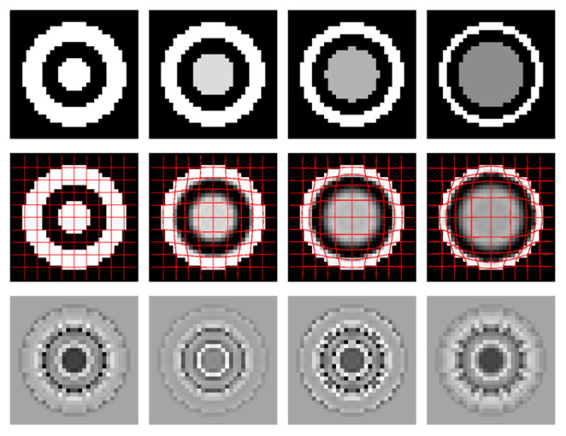
In Fig. 1, four images (32 × 32, spacing 0.04) are synthesized to simulate the movement of a bull’s eye. The outside white loop of the eye shrinks with no intensity changes, while the inside circle grows at a constant speed and its intensity changes from white to gray. The images are at time instants 0, 10, 20, 30 and we chose the first one as the base image. Eight Gaussian kernels [19] are used for K: {K_0.5, K_0.4, K_0.3, K_0.25, K_0.2, K_0.15, K_0.1, K_0.05}; ρ = 0.75. The result confirms that the spatial transformation and intensity changes are captured simultaneously. The dark solid circle at the center of the average momentum of Fig. 1 indicates that the intensity of the inside circle will decrease gradually. The white loop outside of the dark area captures the growth of the inside circle.

Fig 1.

Bull’s eye metamorphic regression experiment. Measurement images (top row). Metamorphic regression result (middle row) and momenta (bottom row). The first image is chosen as base image. Momenta images: left: time-weighted average of the initial momenta; right: momenta of the measurement images with respect to the base image.

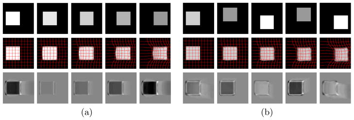
Fig. 2 shows a square (64 × 64; spacing 0.02) moving from left to right at a uniform speed with gradually decreasing intensity. Measurements are at 0, 10, 20, 30, 40. We used a multi-Gaussian kernel K with {K_1.0, K_0.75, K_0.5, K_0.4, K_0.3, K_0.2, K_0.1} and set ρ = 5.0. Metamorphic regression successfully captures the spatial transformation and the intensity changes of the square even when adding vertical oscillations. As expected, metamorphic regression eliminates the oscillations while capturing the intensity change and the movement to the right. We see from the time-weighted average of the initial momenta that intensity changes are controlled by the values inside the square region (dark: decreasing intensity; bright: increasing intensity). The spatial transformations are mainly controlled by the momenta on the edges of the square.

Fig 2.

Square metamorphic regression experiment. (a) moving square with decreasing intensities and no oscillations during movement; (b) moving and oscillating square with alternating intensities. For both cases, the base image is the first one. Top row: measurement images, middle row: metamorphic regression results, bottom row: momenta images (left: time-weighted average of the initial momenta, to the right: momenta of the measurement images with respect to the base image).

7.2 Real Images

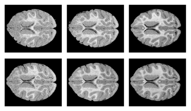
Fig. 3 shows two representative longitudinal MRI time-series (300 × 250 with spacing 0.2734) of nine macaque monkeys at age 3, 6, and 12 months. Some subjects have no visible myelination in the anterior parts of the brain at 3 months (top left), while others show substantial myelination (bottom left). Here, we use metamorphic geodesic regression not for an individual longitudinal image set, but for all nine monkeys and all time-points simultaneously. We use an unbiased atlas for images at 12 months as the base image. Metamorphic geodesic regression is applied over the remaining 18 images at 3 and 6 months. We use a multi-Gaussian kernel, K, with {K₄₀, K₂₀, K₁₅, K₁₀, K₅, K_2.5}; ρ = 500.

Fig 3.

Representative data-sets at 3, 6 and 12 months (left to right)

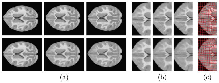
Fig. 4 shows regression results for the simple metamorphic model and for its LDDMM version [9] which cannot capture intensity changes. The metamorphic regression geodesic captures intensity changes of the brain well (increase in white matter intensity with age caused by myelination) while capturing spatial deformations, most notably a subtle expansion of the ventricles.

Fig 4.

Regression results for monkey data: LDDMM (top) metamorphosis (bottom). (a) Images on geodesic at 12, 6, 3 months; (b) Zoom in for images on geodesic at 12, 6, 3 months; (c) Zoom in for images at 3 months to illustrate spatial deformation.

8 Discussion and Conclusions

We proposed metamorphic geodesic regression for image time-series which simultaneously captures spatial deformations and intensity changes. For efficient computations we use a tangent space approximation with respect to a chosen base-image. Solutions can be computed by solving pairwise metamorphosis problems through a shooting approach. Future work will address the properties of the approximation, alternative models of intensity change and the trade-off between spatial deformation and change in image intensities.

References

- 1.Fletcher T. Geodesic regression on Riemannian manifolds. MICCAI Workshop on Mathematical Foundations of Computational Anatomy; 2011. pp. 75–86. [Google Scholar]
- 2.Trouvé A, Vialard F. A second-order model for time-dependent data interpolation: Splines on shape spaces. Workshop STIA-MICCAI; 2010. [Google Scholar]
- 3.Niethammer M, Huang Y, Vialard F-X. Geodesic Regression for Image Time-Series. In: Fichtinger G, Martel A, Peters T, editors. MICCAI 2011, Part II. LNCS. Vol. 6892. Springer; Heidelberg: 2011. pp. 655–662. [DOI] [PMC free article] [PubMed] [Google Scholar]
- 4.Durrleman S, Pennec X, Trouvé A, Gerig G, Ayache N. Spatiotemporal Atlas Estimation for Developmental Delay Detection in Longitudinal Datasets. In: Yang G-Z, Hawkes D, Rueckert D, Noble A, Taylor C, editors. MICCAI 2009, Part I. LNCS. Vol. 5761. Springer; Heidelberg: 2009. pp. 297–304. [DOI] [PMC free article] [PubMed] [Google Scholar]
- 5.Fishbaugh J, Durrleman S, Gerig G. Estimation of Smooth Growth Trajectories with Controlled Acceleration from Time Series Shape Data. In: Fichtinger G, Martel A, Peters T, editors. MICCAI 2011, Part II. LNCS. Vol. 6892. Springer; Heidelberg: 2011. pp. 401–408. [DOI] [PMC free article] [PubMed] [Google Scholar]
- 6.Rohlfing T, Sullivan EV, Pfefferbaum A. Regression Models of Atlas Appearance. In: Prince JL, Pham DL, Myers KJ, editors. IPMI 2009. LNCS. Vol. 5636. Springer; Heidelberg: 2009. pp. 151–162. [DOI] [PMC free article] [PubMed] [Google Scholar]
- 7.Holm DD, Trouvé A, Younes L. The Euler-Poincaré theory of metamorphosis. Quarterly of Applied Mathematics. 2009;67:661–685. [Google Scholar]
- 8.Miller MI, Younes L. Group actions, homeomorphisms, and matching: A general framework. International Journal of Computer Vision. 2001;41:61–84. [Google Scholar]
- 9.Hong Y, Shi Y, Styner M, Sanchez M, Niethammer M. Simple Geodesic Regression for Image Time-Series. In: Dawant BM, Christensen GE, Fitzpatrick JM, Rueckert D, editors. WBIR 2012. LNCS. Vol. 7359. Springer; Heidelberg: 2012. pp. 11–20. [Google Scholar]
- 10.Gupta SN, Prince JL. On variable brightness optical flow for tagged MRI. IPMI. 1995:323–334. [Google Scholar]
- 11.Friston K, Ashburner J, Frith C, Poline J, Heather J, Frackowiak R. Spatial registration and normalization of images. Hum Brain Mapp. 1995;3(3):165–189. [Google Scholar]
- 12.Periaswamy S, Farid H. Elastic registration in the presence of intensity variations. IEEE Trans Med Imaging. 2003;22(7):865–874. doi: 10.1109/TMI.2003.815069. [DOI] [PubMed] [Google Scholar]
- 13.Nocedal J, Wright S. Numerical optimization. Springer; 1999. [Google Scholar]
- 14.Garcin L, Younes L. Geodesic Image Matching: A Wavelet Based Energy Minimization Scheme. In: Rangarajan A, Vemuri BC, Yuille AL, editors. EMMCVPR 2005. LNCS. Vol. 3757. Springer; Heidelberg: 2005. pp. 349–364. [Google Scholar]
- 15.Vialard F, Risser L, Rueckert D, Cotter C. Diffeomorphic 3D image registration via geodesic shooting using an efficient adjoint calculation. International Journal of Computer Vision. 2012;97(2):229–241. [Google Scholar]
- 16.Ashburner J, Friston K. Diffeomorphic registration using geodesic shooting and Gauss-Newton optimization. Neuroimage. 2011;55(3):954–967. doi: 10.1016/j.neuroimage.2010.12.049. [DOI] [PMC free article] [PubMed] [Google Scholar]
- 17.Beg M, Miller M, Trouvé A, Younes L. Computing large deformation metric mappings via geodesic flows of diffeomorphisms. IJCV. 2005;61(2):139–157. [Google Scholar]
- 18.Hart GL, Zach C, Niethammer M. An optimal control approach for deformable registration. MMBIA. 2009:9–16. [Google Scholar]
- 19.Risser L, Vialard F, Wolz R, Murgasova M, Holm D, Rueckert D. Simultaneous multiscale registration using large deformation diffeomorphic metric mapping. IEEE Transactions on Medical Imaging. 2011;30(10):1746–1759. doi: 10.1109/TMI.2011.2146787. [DOI] [PubMed] [Google Scholar]