

Abstract
Routine monitoring along the coast of the Gulf of Maine (GoM) reveals shellfish toxicity nearly every summer, but at varying times, locations, and magnitudes. The responsible toxin is known to be produced by the dinoflagellate Alexandrium fundyense, yet there is little apparent association between Alexandrium abundance and shellfish toxicity. One possibility is that toxic cells are persistent in offshore areas and variability in shellfish toxicity is caused not by changes in overall abundance, but rather by variability in transport processes. Measurements of offshore Alexandrium biomass are scarce, so we bypass cell abundance as an explanatory variable and focus instead on the relations between shellfish toxicity and concurrent metrics of GoM meteorology, hydrology, and oceanography. While this yields over two decades (1985–2005) of data representing a variety of interannual conditions, the toxicity data are gappy in spatial and temporal coverage. We address this through a combination of parametric curve fitting and hierarchical cluster analysis to reveal eight archetypical modes of seasonal toxicity timing. Groups of locations are then formed that have similar interannual patterns in these archetypes. Finally, the interannual patterns within each group are related to available environmental metrics using classification trees. Results indicate that a weak cross-shore sea surface temperature (SST) gradient in the summer is the strongest correlate of shellfish toxicity, likely by signifying a hydrological connection between offshore Alexandrium populations and near-shore shellfish beds. High cumulative downwelling wind strength early in the season is revealed as a precursor consistent with this mechanism. Although previous studies suggest that alongshore transport is important in moving Alexandrium from the eastern to western GoM, alongshore SST gradient is not an important correlate of toxicity in our study. We conclude by discussing the implications of our results for designing efficient and effective shellfish monitoring programs along the GoM coast.
Keywords: harmful algal blooms, red tides, paralytic shellfish poisoning, cluster analysis, CART modeling, satellite remote sensing
1. Introduction
The Gulf of Maine (GoM) coast (Figure 1) is plagued by annually recurring shellfish toxicity caused by the dinoflagellate Alexandrium fundeyense (Shumway et al., 1988). Filterfeeding shellfish accumulate the toxin produced by Alexandrium and present a health risk to humans in the form of paralytic shellfish poisoning (PSP), a potentially fatal condition (Etheridge, 2010). For this reason, management agencies of Maine, New Hampshire, and Massachusetts have monitored shellfish toxicity levels along the GoM coast for 30+ years. Shellfish beds with toxin levels approaching or exceeding 80 μg toxin/100 g shellfish tissue are closed to harvesting, often resulting in significant economic losses. The summer of 2005 was especially severe, resulting in harvesting closures from the central Maine coast south through Massachusetts, as well as 40,000 km2 of federal offshore resources (Anderson et al., 2005a; Jin et al., 2008).
Figure 1.

Map of the coastal Gulf of Maine showing relevant landmarks, dominant surface circulation patterns (grey arrows), and positions of shellfish sampling locations for both Mytilus and Mya.
In other coastal systems, relationships have been identified between Alexandrium abundance and shellfish toxicity. For example, in the Estuary and Gulf of St. Lawrence, toxicity of the blue mussel, Mytilus edulis, was found to correspond geographically with the distribution of Alexandrium tamarense (Blasco et al. 2003). Additionally, over the four years of available data, 32% of the variability in the magnitude of toxicity was accounted for by A. tamarense abundance. In the Puget Sound, shellfish toxicity was found to be preceded by an increase in Alexandrium catenella cells in 71% of cases (Dyhrman et al. 2010). Further, an annual index of shellfish toxicity was found to covary with an index of the Pacific Decadal Oscillation (PDO) as well as with the number of days per year that sea surface temperature exceeded 13°C (Moore et al. 2010). In the GoM, such clear mechanistic or statistical associations between Alexandrium fundeyense cell abundance or distribution and the timing, location, or magnitude of coastal shellfish toxicity events have yet to be demonstrated. In part, this may be due to the relatively few and only recent comprehensive surveys of Alexandrium cell distribution in the GoM (e.g. Townsend et al., 2001) and the fact that, in those years of available data, the mean Alexandrium abundance has been surprisingly stable (McGillicuddy et al., 2005). This suggests that interannual variation in shellfish toxicity may be determined not only by the actual abundance of offshore Alexandrium, but also by the relative effectiveness with which these populations are delivered to the coastal zone (McGillicuddy et al., 2005, 2011; Stock et al., 2007). This hypothesis is supported by short-term studies linking episodic transport phenomena and specific algal bloom or toxicity events in the western GoM (Keafer et al., 2005; Luersson et al., 2005; Li et al., 2009; McGillicuddy et al., 2011). Thomas et al. (2010) compared interannual variability in mean toxicity within groups of statistically similar sampling locations to environmental data, showing that groups in the western GoM tend to be positively correlated with wind stress and sea surface temperature patterns that indicate onshore transport and coastal downwelling.
In this study, we systematically investigate the ‘persistant abundance and fluctuating transport’ hypothesis of Alexandrium-induced shellfish toxicity in the GoM by statistically relating 21 contiguous years of quantitative coastal shellfish toxicity data to concurrent environmental metrics that are indicative of GoM surface circulation.
The use of monitoring data collected by state agencies primarily for the purpose of protecting public health, rather than for testing scientific hypotheses, raises some methodological challenges (Thomas et al., 2010). Individual locations are sampled neither regularly nor randomly in space and time. Sampling frequency and location have been adjusted both within any given year and across years in response to emerging patterns of toxicity. The complexity of the GoM coastline and the observed patchiness of Alexandrium cell abundance (Crespo et al. 2011) means that any method of averaging or otherwise combining observations across space and time cannot be substantiated a priori, but rather must be based on the results of appropriate statistical analysis.
In previous work, Thomas et al. (2010) addressed the issue of gappy coverage at individual locations in the shellfish data by using multivariate clustering to group stations with similar interannual toxicity records and forming averages within groups. This methodology was applied to six succinct metrics of annual toxicity (defined with reference to the 80 μg toxin/100 g shellfish tissue threshold value): date of first toxicity, duration of toxicity, magnitude of maximum toxicity, total annual toxicity, date of maximum toxicity, and presence/absence of toxicity. We expand on the results of Thomas et al. (2010) using an extended data set and a different approach. We fit parametric curves to all data from each location-year combination. This holistic characterization provides a portrayal of a year’s complete toxicity pattern at each location. Conceptually, such a characterization also provides robustness to missing data and changes in sampling patterns while avoiding sensitivity to any particular toxicity threshold employed. We then identify archetypical timing patterns of seasonal toxicity across all years and locations providing additional insights to those of Thomas et al. (2010) concerning seasonality and the identification of anomalous years and locations. These archetypes are next used to form groups of locations that have similar interannual patterns. The interannual patterns within each group are then related to interannual differences in available environmental and oceanographic variables. We explore beyond the simple bivariate correlations of Thomas et al. (2010), considering multiple independent variables simultaneously and allowing for the possibility of threshold effects and variable interactions. To do this, we use a classification and regression tree (CART) approach (Breiman et al., 1984). To our knowledge, this is the first application of CART, a very flexible and easily interpretable statistical procedure, to the modeling of shellfish toxicity (see Gannon et al., 2009 for a recent application of CART modeling to toxic algal blooms and fish catch). We apply these tools to toxicity data from both blue mussels (Mytilus edulis) and softshell clams (Mya arenaria) collected by the states of Maine, New Hampshire and Massachusetts to yield results as widely applicable as possible to shellfish monitoring programs along the GoM coast.
2. Description of Study Area
Toxicity in GoM shellfish has been recorded in eastern Maine locations since at least 1958, and almost annually along the greater GoM coast since 1972 (Hurst, 1975). This toxicity has strong seasonality, being restricted to the summer (Hurst and Yentsch, 1981; Shumway et al., 1988) and generally occurring earlier west of Penobscot Bay than to the east (McGillicuddy et al., 2005; Thomas et al., 2010). However, within this overall pattern, there is substantial variability in the timing, duration and strength of toxicity peaks, even between locations that have close geographic proximity (Franks and Anderson, 1992; Anderson et al., 2005a; Bean et al., 2005; Thomas et al., 2010). This makes it difficult to identify consistent spatial or temporal patterns.
Scientific efforts over the past decade have strongly improved our understanding of the oceanographic ecology of Alexandrium (Anderson et al., 2005; Anderson et al., 2012). Cells appear to be broadly present offshore, in distributions linked to circulation patterns (Townsend et al., 2001, 2005). Growth appears limited by temperature throughout the Gulf in the early spring and by nutrients in the western Gulf in summer. This would explain the observed seasonal timing of toxicity: population growth is generally more rapid in the west early in the summer due to warmer temperatures, but more rapid in the east later in the summer due to nutrient limitation in the west. Beyond this seasonal regularity, a clear link between offshore Alexandrium cell patterns and coastal shellfish toxicity remains elusive. If Alexandrium populations in the open GoM are the dominant source of coastal toxicity, then shellfish contamination requires two conditions: (i) toxic Alexandrium cells need to be present in sufficient numbers and (ii) the cells need to come in contact with shellfish. Thus, the physical transport of cells is a key component to understanding and anticipating shellfish toxicity.
On a broad scale, surface transport patterns in the GoM are well-known (Figure 1). Circulation predominantly consists of a counterclockwise gyre, the westward flowing coastal portion of which is referred to as the Maine Coastal Current (MCC) (Brooks, 1985). This is divided into a colder, stronger and more persistent Eastern Maine Coastal Current (EMCC) between the Canadian border and Penobscot Bay (Figure 1) and a weaker, more variable and seasonally stratified Western Maine Coastal Current (WMCC) west of Penobscot Bay. Large Alexandrium cyst beds are known to exist in the Bay of Fundy just upstream from the Maine coast (Martin and White, 1988), and further west off Casco Bay (Anderson et al., 2005), both providing possible source populations for the coastal GoM, delivered annually by the MCC (Townsend et al., 2001; Anderson et al., 2005). However, there is significant variability in the extent of alongshore transport. During summer, a portion of the EMCC often branches offshore at Penobscot Bay to recirculate around Jordan Basin (Brooks and Townsend, 1989). The diminished remainder is then joined by freshwater input from Maine rivers to form the Western Maine Coastal Current (WMCC) (Churchill et al., 2005; Pettigrew et al., 2005). The WMCC continues around Wilkinson basin, toward the western Maine shore and the coasts of New Hampshire and Massachusetts. This implies that the potential for shellfish toxicity in the western GoM may be related to the strength of both the WMCC and the EMCC and their relative connection (Luerssen et al., 2005; Pettigrew et al., 2005).
The extent of branching of the MCC near Penobscot and the subsequent interaction of the WMCC with the western coast itself is thought to be regulated by a combination of river runoff and wind stress (Anderson et al., 2005c). Downwelling-favorable conditions are believed to hold the plume and any toxic cells it contains against the coast and accelerate it alongshore, spreading the potential for contamination of shellfish beds to the west (Franks and Anderson, 1992). Upwelling conditions seem to retard progression of the plume, slowing spread of Alexandrium cells and eventually transporting them offshore (Keafer et al., 2005).
The basic premises of the above hypotheses have been supported by episodic data from cruises and moored instrumentation. For example, Keafer et al. (2005) found that downwelling winds were associated with Alexandrium bloom formation and increased shellfish toxicity in 1998, while upwelling winds were associated with low near-shore cell abundance and decreased toxicity in 2000 (Keafer et al., 2005). Analysis of 13 years of shellfish data collected at 8 locations along the western Maine coast (Luerssen et al., 2005) suggests a link between interannual variability in toxicity and differences in the timing and strength of the temperature front separating the relatively cold EMCC from the warmer water of the WMCC. However, this relationship was not supported by the more extensive analysis of Thomas et al. (2010), although years of increased onshore wind stress and reduced cross-shore temperature gradients were shown to be those years of increased coastal toxicity along the western Maine coast.
3. Data and Methods
3.1 Shellfish Toxicity Data
Shellfish toxicity data were received from the Maine Department of Marine Resources, the Massachusetts Division of Marine Fisheries, and the New Hampshire Department of Environmental Resources. This compilation of toxicity records for the 21-year period of 1985 to 2005 has over 90,000 records from 450 different coastal locations along the GoM coast. At some “primary” locations, sampling occurs approximately weekly (Bean et al., 2005). However, the nature of state monitoring programs means that the sampling frequency at most locations varied over the 21-year period, creating many spatial and temporal gaps. Toxicity in this record was measured in more than ten different species of shellfish, but blue mussels (Mytilus edulis) and softshell clams (Mya arenaria), comprise about 60% and 22% of the records, respectively. To provide the most robust, broad and consistent time/space coverage possible, we limit our study to these two species, keeping them separate for statistical analysis.
3.2 Toxicity Data Curve Fitting
To fill gaps in the shellfish toxicity records, we first fit smooth curves to the data of each location-year combination. Location-year combinations with fewer than eight individual observations were discarded. A total of 1347 location-year combinations for Mytilus and 810 for Mya (comprising 19392 and 7990 individual measurements, respectively) had sufficient data for curve-fitting. We considered a variety of three-parameter peak functions, including the Gaussian, Lorentzian, Logistic, Complementary Error Function, and Laplace, as well as some with an additional parameter controlling the shape of the peak, including the Modified Gaussian, Pearson VII, Triangular, Error Function, Gaussian-Lorentzian Cross Product, Symmetric Double Sigmoidal, and Symmetric Double Gaussian. The sum of the squared differences between the fitted curve and the measured toxicity for each location-year combination was used as the fitting criterion, and the Gaussian was thereby found to be the best-fitting functional form. Each location-year combination was allowed to have as many as two separate Gaussian peaks, as determined by the Bayesian Information Criterion (Schwarz, 1978)
3.3 Identifying Archetypical Seasonal Timing Patterns
A cluster analysis on all individual location-year combinations was used to identify archetypical seasonal patterns in the data sets for each of the two species. To focus on the relative timing of toxicity, rather than the strongly variable magnitude, toxicity curves were first normalized by dividing by the peak toxicity for that year and location. Similarity was based on the sum of the squared differences between interpolated daily values of the respective normalized seasonal toxicity curves. We used a hierarchical clustering method, as implemented by the hclust function in R v2.0 (R Development Core Team, 2011). This function uses an agglomerative algorithm to cluster objects based on a specified measure of dissimilarity. We chose Ward’s method of agglomeration (Ward, 1963), in which each object is initially assigned to its own cluster. The algorithm then proceeds iteratively, at each stage joining the two most similar clusters until there is a single cluster. Dissimilarity between two clusters at each step is computed as the increase in the “error sum of squares” (ESS) that would result from aggregating two clusters into a single cluster. Ward’s method chooses successive clustering steps so as to minimize the increase in the ESS at each step.
Hierarchical clustering results are conveniently visualized as a dendrogram, with the length of the branches representing the distance between adjacent clusters. This provides a graphical basis for choosing the number of clusters that would result from cutting the dendogram at a particular height (Langfelder et al., 2007). While a number of metrics are available for evaluating the relative merits of different cut heights, we made a subjective choice to yield a reasonable number of groups while visually maximizing inter-group differences relative to intra-group differences. The resulting location-year groupings of seasonal toxicity patterns are henceforth referred to as T-groups and denoted with numbers.
3.4 Grouping Locations According to Interannual Patterns
To identify locations with similar interannual variability of seasonal toxicity, locations were next clustered according to T-group membership patterns across all 21 years. The distance metric used in this case was the binary dissimilarity of T-group membership between locations for each year (i.e., T-group membership is compared between any two locations for each year; if they are different, the distance is 1, else it is 0). To maximize the robustness of our between-location distance measure, locations with T-group assignments for fewer than 50% (12 out of 21) of the years were discarded.
The dendrogram produced by hclust was cut to define distinct groups of locations. Again, the number of groups was a subjective choice, intended to yield neither too many nor too few groups, with reasonable cohesiveness apparent in each group. These groups reflect spatial arrangements of locations along the GoM coast with similar interannual variability in seasonal toxicity patterns and are henceforth referred to as S-Groups and denoted with capital letters.
3.5 Selection and Construction of Environmental Forcing Variables
Relatively few environmental variables that are consistently measured through each season are available over the full 21 years of available toxicity data. Satellite-measured sea surface temperature (SST) data are available from the National Oceanic and Atmospheric Administration (NOAA) from 1985 to the present. These images were processed as described by Thomas et al. (2010) to provide metrics of temperature patterns indicative of surface circulation in the GoM. Briefly, the maximum alongshore SST gradient (ASST) was extracted from monthly averaged SST composites as a metric of connectivity through the frontal region off Penobscot Bay separating the colder water of EMCC from the warmer water of the WMCC. A high value of the ASST indicates a strong temperature front and a weak alongshore connection, while a low value indicates a weak front and a stronger connection. For the shorter cross-shore transect running offshore from the coast toward Wilkinson Basin, the cross-shore SST slope (XSST) of monthly averaged composites was used as an indicator of continuity between near-shore and off-shore surface water masses. A positive value of the slope indicates colder water near the coast compared to offshore and is indicative of upwelling and a weaker (or absent) surface connection between inshore and offshore waters.
NOAA records wind speed and direction hourly at Matinicus Rock (Fig. 1). On the time scales we investigate here, winds at this location can be considered to be generally representative of conditions along the GoM coast. The wind speed data were converted to monthly cumulative wind stress in upwelling-favorable (UWIND) and downwelling-favorable (DWIND) directions as described by Thomas et al. (2010). Monthly cumulative values are used in an attempt to capture the long-term wind-forcing history.
From west to east, the major freshwater discharges to the GoM include the Androscoggin, Kennebec, and Penobscot Rivers. The Penobscot is the largest of the three in terms of both watershed size and average discharge, and a preliminary analysis showed that the timing of its discharge is strongly correlated with that of the other major rivers. Therefore monthly average discharge from the Penobscot was used as a representative metric for interannual variability in coastal freshwater input. Daily discharge data were obtained from the United States Geological Survey (USGS).
3.6 Model Construction
Classification and regression tree (CART) methods were applied to each S-group of locations to relate the interannual patterns in T-group membership to the meteorological, hydrologic, and oceanographic forcing variables. CART models consist of dichotomous splits of predictor variables so as to yield the strongest associations with the dependent variable. This splitting process continues sequentially until a specified stopping criterion is met (e.g., a minimum number of observations that must remain at a node for a further split to be attempted; a minimum factor by which the lack of fit must be reduced by an attempted split; a maximum number of nodes allowed on any path through the tree).
CART models are represented as (inverted) trees, with all observations present at the (top) root node. At the point of the first split, the branch to the left indicates agreement with the revealed dichotomous condition and the branch to the right indicates disagreement. The next two splits are then attempted, each conditional on the result of the first split. When the stopping criterion is met, the most likely value of the dependent variable is reported at the endpoints, or leaves, of the final branches. The lengths of the branches are proportional to the amount of variation in the dependent variable accounted for by the previous split. When the dependent variable belongs to a category or class (as is the case for our T-groups), the statistical methods are those of classification and results can be evaluated using error rates (Breiman et al., 1984). When the dependent variable is continuous, the statistical methods are those of least-squares regression and the conditional standard deviations can be evaluated.
CART methods do not require the partitioning variables to follow any specific type of distribution, nor do they assume linearity in the relationships (Feldesman, 2002). Partitioning variables can be categorical, interval-valued, continuous, or any combination thereof (Clark et al., 1992; Yohannes and Hoddinott, 1999). The sequential nature of splits captures underlying nonlinear relationships as well as interactions between variables (Breiman et al., 1984). CART methods are also invariant under monotone transformations of the partitioning variables (Yohannes and Hoddinott, 2006).
Our CART models are implemented using the R function rpart (Therneau and Atkinson, 2008). We chose a stopping rule that empirically provided concise and interpretable models that did not seem to merely reflect noise in the data (Han and Kamber, 2006). Specifically, splits were maintained only if they reduced the lack of fit of the model by at least 0.04/n, where n = the number of locations in the S-group being modeled. We also limited the overall depth of the trees to three nodes to avoid having more than eight combinations of conditions, which we expected to be difficult to interpret.
3.7 Model Validation
To maximize statistical power, the CART models were developed using all available data. Therefore, model testing was performed for each S-group using cross-validation. For each year, a model was fitted to all other years and then used to generate a prediction for the excluded year. Predictions consisted of T-group membership and were evaluated in two ways: (i) with regard to the accuracy of predicting the particular T-group membership and (ii) with regard to the accuracy of predicting the occurrence of any toxicity in that year (any T-group other than the one representing non-toxicity). For the former, we used both the overall predictive accuracy (PA = correct predictions / N, where N = the total number of location-year combinations) and a modified version of the Heidke Skill Score (Heidke, 1926) for multinomial predictions (MHSS = [(correct predictions – expected correct) / (N – expected correct)], where the expected number of correct predictions is the number that would be correct if the most common observed T-group were predicted for every location-year combination. Thus, the HSS measures the fractional improvement of the model over a ‘default’ forecast. For the binomial toxicity prediction, we used the probability of detection (POD = correct positives / (correct positives + false negatives)), the false alarm ratio (FAR = false positives / (correct positives + false negatives)), the critical success index (CSI = correct positives / (correct positives + false positives + false negatives), also referred to as the threat score, and the original Heidke Skill Score (in which the expected number of correct predictions is the number that would be correct by chance if toxicity were predicted at historical frequencies).
4. Results
4.1 Archetypical Seasonal Patterns of Toxicity
A Gaussian function allowing for as many as two peaks per year (Figure 2) provided a very good overall fit to the toxicity data (overall R2=0.94, n=27382). The fitted parameters for each location-year combination consist of the height of the peak(s), the year-day of the middle of each peak, and the width of each peak. These parameters can be used to impute estimated toxicity values for any day of the year for any location-year combination.
Figure 2.

Representative two-peak Gaussian curve fit to Mytilus data collected in 1990 at Basin Point, ME. This location-year combination represents one of the 2157 seasonal toxicity patterns analyzed in this study.
Hierarchical clustering applied to the normalized toxicity curves of each location-year combination indicates that eight archetypical patterns (T-groups) are appropriate for both Mytilus and Mya (dendrograms not shown due to their size). These groups represent common seasonal patterns across all locations and years for each species. It is clear from plots of these curves (Figures 3 and 4) that, depending on the year and location, toxicity may either: not occur at all (T1), start early and stay long (T2), start and end early and then occur again (T3), occur only briefly in early- or late-summer (T4, T6), occur for prolonged periods in mid-summer (T5), possibly even occurring twice (T7), or start late in the summer and remain toxic well into autumn (T8).
Figure 3.

Groupings of normalised seasonal toxicity patterns (T-groups) across all location-year combinations for Mytilus. Dark grey curves represent the first (or only) fitted peak; light grey curves represent the second fitted peak when appropriate; bold black curves represent the average seasonal pattern across all location-year combinations in each T-group. Group designations and sample size (location-year combinations) are also shown for each T-group.
Figure 4.

Groupings of normalised seasonal toxicity patterns (T-groups) across all location-year combinations for Mya. Dark grey curves represent the first (or only) fitted peak; light grey curves represent the second fitted peak when appropriate; bold black curves represent the average seasonal pattern across all location-year combinations in each T-group. Group designations and sample size (location-year combinations) are also shown for each T-group.
4.2 Groups of Locations According to Interannual Patterns
Hierarchical cluster analysis applied to the interannual patterns in T-group membership of each location suggests that five spatial S-groups are appropriate for the Mytilus toxicity data (Figure 5). S-group A examination of the interannual pattern of T-groups reveals that these locations exhibit late-season toxicity patterns T6, T7, and T8 in most years, although in the late 1990’s many of these locations experienced either no toxicity (T1) or prolonged mid-season toxicity (T5). The years 1985, 1987, and 2002–2004 are distinct in S-group A in experiencing only a single, very late-season toxicity peak (T8) at most locations.
Figure 5.
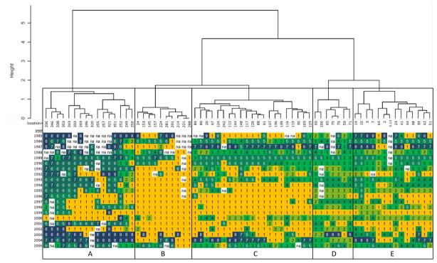
Cluster dendrogram for Mytilus showing grouping of sampling locations (S-groups) according to interannual patterns in T-group occurrence. Lengths of branches represent the dissimilarity between adjacent clusters. End branches are labeled with location numbers, below which is shown a matrix of T-group membership by location and year. T-group membership is indicated by numbers corresponding to Figure 3, as well as grey-shading to visually emphasize patterns across years and locations. Missing values are indicated by ‘na’. The tree was subjectively cut at a height of 1.5 to yield five groups identified by capital letters.
The locations in Mytilus S-group B are mostly non-toxic (T1), although in some years locations experienced a single peak of toxicity (T5 or T6). S-group C consists of locations that experienced early and mid-season toxicity (T3 and T5) in the late 1980’s, 1990, 1993, and 2000, and 2005. Except for these years, the 1990’s were mostly non-toxic (T1) for these locations. The years 1987, 2003, and 2004 stand out for experiencing toxicity late in the season (T7 and T8).
Mytilus S-groups D and E are fairly similar to one another, experiencing mostly early-season T-groups T2, T3, and T4. The year 1987 stands out in both groups as having later toxicity (T7 or T8), while group E also experienced late-season toxicity in 1985 and 2004. In S-group E, the year 2005 is notable in having many locations with a double-peaked toxicity pattern (T3) that had not occurred to any significant degree since the early 1990’s.
A mapping of the Mytilus sampling locations identified by S-group (Figure 7, top) shows a strong degree of geographical coherence. The locations of group A lie exclusively in the far east near the Bay of Fundy, while those in group B are mostly located around Penobscot Bay. With the exception of one location to the east and two to the west, those of group C lie between Penobscot and Casco Bays. The locations in group D are mostly within Casco Bay, while those of E are also in Casco Bay as well as further west into New Hampshire.
Figure 7.

Map showing Mytilus (top) and Mya (bottom) sampling locations grouped according to interannual patterns of seasonal toxicity (S-Groups) as identified in Figures 5 and 6, respectively.
For the Mya data, cluster analysis suggests that only three groups of locations are clearly distinguishable at a cut height of 1.5 (Figure 6). Mya S-group A is distinct from the other groups by the predominance of late season toxicity patterns T5 through T8, with the late 1990’s characterized by no toxicity (T1) or mid-season toxicity (T4). The year 2003 stands out as the only year with very late toxicity group T8. Mya S-group A has similar interannual variability to Mytilus S-group A.
Figure 6.

Cluster dendrogram for Mya showing grouping of sampling locations (S-groups) according to interannual patterns in T-group occurrence. T-group membership is indicated by numbers corresponding to Figure 4. All other notation is the same as in Figure 5.
The locations in Mya S-group B are mostly non-toxic (T1), although many locations experienced a single peak of toxicity (T4 or T6) in the same years as Mytilus S-group B. Mya S-group C experienced similar toxicity patterns in these same years, but also in 1993 through 1995. These locations experienced unusual double peaks (T3) in 1988, 1991, and 2005. The years 1987, 2003, and 2004 were unusual in the occurrence of very late-season peaks (T7 and T8) in both S-groups B and C.
A map of the Mya sampling locations (Figure 7, bottom) also reveals strong geographic coherence. S-group A consists exclusively of locations near the Bay of Fundy. No other locations east of Penobscot Bay had sufficient sampling for inclusion in our analysis. Mya S-group B locations lie just west of Penobscot Bay and along the west of Casco Bay. The locations of group C are on the east side of Casco Bay and further west along the Maine coast towards New Hampshire.
Averaged within each Mytilus S-group, the date of peak toxicity in each year shows systematic geographic differences consistent with previous work and highlights the interannual patterns (Figure 8). Western groups D and E typically exhibit the earliest peaks, with eastern S-group A peaking approximately a month later. Interannual variation in timing is largely spatially synchronous among groups C, D, and E, with ‘late’ toxicity years (e.g. 1985, 1987, 2003, 2004) peaking late in most groups. There is no obvious long term trend in the timing of peaks, although 2003 stands out with especially late toxicity in most S-groups.
Figure 8.

Interannual variability in peak toxicity timing for Mytilus S-groups. Points indicate date (year-day) of seasonal peak toxicity averaged across locations in each S-group, plotted by year. Missing points indicate years without toxicity. Symbols shown in the legend are the same as those used in the maps. To conserve space, plots for Mya are not shown. Temporal patterns for Mya are similar to those for Mytilus.
4.3. Relations with Environmental Forcing Variables
Toxicity patterns in the eastern S-groups A and B for both Mytilus and Mya are of less management interest than the western locations, because of their historically late and very low toxicity, respectively. Therefore, we focus our subsequent analysis on S-groups C, D, and E for Mytilus and S-group C for Mya. Figure 8 shows significant interannual variation in the timing of shellfish toxicity within each of these groups. This temporal variation, as characterized by T-group membership across years (see Figs. 5 and 6), serves as the response to be explained by the candidate environmental variables using CART modeling. We develop a separate CART model for each S-group of locations (Figure 9), the results of which can be read directly from the trees. For example, for Mytilus S-group C, July cross-shore SST gradient (July.XSST) off western Maine is the first node in the tree, indicating that it has the strongest overall association with T-group membership. When this metric is less than 0.004236 (indicating a relatively strong cross-shore hydrologic connection), July.XSST again acts as the next dichotomous variable, so that if July.XSST is less than 0.002614, single-peak group T5 is expected, otherwise double-peak group T7 is expected. When July.XSST is greater than 0.004236 (indicating a weaker cross-shore connection), June downwelling wind (June.DWIND) acts as the next partitioning variable, with values less negative than −0.2452 (indicating weak downwelling winds) leading to non-toxic group T1 and greater values implying double-peak group T3. The trees for the other S-groups of locations can be interpreted similarly.
Figure 9.
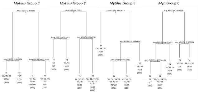
Classification trees for S-groups west of Penobscot Bay. Each node is identified by a dichotomous split of an environmental variable that yields the strongest association with T-group membership across years. The branch to the left indicates agreement with the stated condition, and the branch to the right indicates disagreement. The lengths of the branches are proportional to the amount of variation explained by the previous split. The most likely T-group is reported at each leaf, as well as the specific years in the 21-year historical record that meet the conditions leading to that leaf. Model accuracy is also reported at each leaf, expressed as the fraction of total location-year combinations correctly identified. The percentage accuracy is also given in parentheses. Variable names and group designations are defined in the text.
While July.XSST was revealed as having the strongest association with toxicity patterns for all Mytilus S-groups, for Mya S-group C July upwelling wind (July.UWIND) was empirically selected as the topmost node. However, July.XSST is also an excellent first partitioning variable and only marginally worse than July.UWIND. To provide consistency across all trees, July.XSST was selected for the first node in this tree as well. Given that both metrics are indicators of July cross-shore connectivity, this substitution does not change the interpretation of results.
Accuracies for each leaf of the trees range from 30 to 100%. Accuracies are typically greater than 50%, except when double-peaked T3 is expected. This seems to be because either of the two constituting peaks (T2 and T4) may be absent in any given year or location (Figure 5). Overall S-group accuracies are: 64% (Mytilus Group C), 55% (Mytilus Group D), 48% (Mytilus Group E), and 60% (Mya Group C).
4.4 Cross-Validation Results
The overall model accuracies (MA) for the cross-validation exercises (Table 1) are similar to those obtained for the CART models fitted to the full data (Fig. 9), indicating model robustness. The Multinomial Heidke Skill Score (MHSS) shows that the model yields about a 30% improvement over the default T-group prediction for most S-groups of locations. Regarding the binomial (toxicity/no toxicity) cross validation tests, the model yields high probabilities of detection (POD) and low false alarm rates (FAR). The critical success index (CSI), which accounts for both false alarms and missed events, is high for all S-groups. The binomial Heidke Skill Score (HSS) indicates generally strong improvements over the number of predictions expected to be correct when simply using historical frequencies in all groups except Mytilus S-group D. This group is toxic at nearly all locations and years, giving little room for improvement over simply predicting ‘toxic’ conditions most of the time. Overall, the two species of shellfish, Mytilus and Mya, do not differ noticeably in their cross-validation results.
Table 1.
Cross-validation results
| Metric | S-Group | ||||
|---|---|---|---|---|---|
| Mytilus C | Mytilus D | Mytilus E | Mya C | ||
| Multinomial | MA | 0.64 | 0.53 | 0.45 | 0.54 |
| MHSS | 0.32 | 0.30 | 0.19 | 0.33 | |
| Binomial | POD | 0.67 | 0.97 | 0.69 | 0.62 |
| FAR | 0.08 | 0.02 | 0.15 | 0.01 | |
| CSI | 0.64 | 0.95 | 0.62 | 0.56 | |
| HSS | 0.66 | 0.16 | 0.49 | 0.61 | |
5. Discussion
Fitting parametric curves to the shellfish toxicity data allowed us to interpolate between measured dates and thereby estimate peak height, date of peak, and overall duration of toxicity for every location-year combination, even when sampling did not coincide with the highest toxin values. We implicitly assumed in our curve-fitting procedure that there was no systematic bias toward missing toxicity peaks, a reasonable assumption given the monitoring objectives of the state agencies. The high R2 value (0.94) for both species indicates that the two-peak Gaussian form is sufficient to capture most of the variability present in the data.
Although our choice of the number of groups arising from the subsequent clustering was somewhat subjective, the resulting eight groups of toxicity timing (T-groups) for each shellfish species appear to be well clustered within each group and distinctly different across groups. Further, no single characteristic is responsible for the assignment of groups. For example, Mytilus groups T4 and T5 have similar average dates of peak toxicity, but are distinguishable by the width of their toxicity peaks. Similarly, Mytilus groups T7 and T8 have overlapping peak timing, but T7 consists mostly of double-peak location-year combinations while those in T8 are mostly single-peaked. These observations support the utility of our holistic approach to toxicity seasonal assessment based on a concise set of archetypical seasonal patterns for each species.
5.1 Interspecies Comparison
The corresponding T-groups for Mya and Mytilus are similar (Figures 3 and 4). However, the toxicity peak tends to occur an average of two weeks later for Mya, and peak toxicity levels tend to be about one third as high. This is consistent with a lower ingestion/accumulation rate and/or higher depuration rate (Bricelj and Shumway, 1998; Duinker et al., 2007; Vasconcelos, 1995; Cusson et al., 2005) and is also consistent with the results of other comparative studies (Blasco et al. 2003). Such results argue against a priori aggregation of the Mya and Mytilus data, and suggest that Mytilus is a more appropriate sentinel species.
5.2 Geographic Coherence
The S-groups of locations with similar interannual patterns (T-groups) reveal some clear spatial and temporal patterns. Most notably, locations that group together are generally in close geographic proximity (Fig. 7), consistent with the results of Thomas et al. (2010) and supporting their contention that many of the factors that drive toxicity patterns are regional. For example, locations in the far eastern part of the Gulf (S-groups A for both Mytilus and Mya) are subject to lower temperatures for longer periods of time. This would reduce growth rates of Alexandrium cells, possibly explaining the predominance of late-arriving peaks (Fig. 8). The fact that these locations are also close to known cyst beds in the Bay of Fundy may account for the higher frequency of toxic years than at most western locations. In contrast, the S-groups of locations in the western region (C, D, and E) are subject to warmer and more variable temperature and circulation patterns, consistent with the generally earlier peaks of toxicity (Fig. 8) and a more diverse set of T-group patterns (Fig. 5).
The identification of a largely non-toxic group of locations (S-group B for both species) is consistent with the historical observation of a ‘PSP-sandwich’ – the phenomenon of much lower or absent toxicity in the area around Penobscot Bay even when adjacent areas are toxic (Hurst and Yentsch, 1981; Shumway et al., 1988). This has been attributed to the role of the Penobscot River in deflecting the EMCC away from the coast (Townsend et al., 2001). Hydrology may also influence toxicity patterns of Mytilus group D locations, mostly within Casco Bay. These locations generally exhibit the earliest toxicity of our five S-groups (Fig. 8) and are known as local ‘hotspots’. It has been suggested that this is due to entrainment of Alexandrium cells delivered from the eastern GOM, rather than the existence of a local source population (Keafer et al., 2005). By demonstrating a strong correspondence between years of toxicity and the strength of offshore connectivity, our CART model results support this suggestion, as discussed further below.
Not all members of each S-group are strictly contiguous, indicating that local hydrology, growing conditions, and/or shoreline orientation can be as important as the regional setting in determining toxicity patterns. For example within the Mytilus data, location #106 clusters with group D (Fig. 5) but is geographically in the midst of group C (Fig. 7, top), perhaps because it is deeper inside Boothbay Harbor than its neighbors and behaves more like the Casco Bay locations. Similarly, group C includes two locations to the west of Casco Bay (#20 and 30) (Fig. 7, top). Closer inspection reveals that these are both especially well-protected by adjacent coastal features, possibly explaining their lower frequency of toxicity than adjacent group E locations.
5.3 Timing of Environmental Forcing
The classification trees for the four S-groups of locations west of Penobscot Bay all show July cross-shore SST gradient to be strongly associated with T-group patterns (Fig. 9). June downwelling wind strength also appears in three of the trees. River flow in April and cross-shore SST gradient in May and June serve as additional, lower-level partitioning variables. Although not shown in the trees, the rpart function also reports those variables that may yield nearly equivalent partitions at each node. Investigation of these alternatives can help guard against fitting of trees to statistical anomalies. While there were occasions in which different variables may have been selected at some nodes without significant loss of accuracy, the consistent appearance of July.XSST and June.DWIND as dominant partitioning variables across the four S-groups analyzed indicates the robustness of the results with respect to these variables.
To better understand the relationships described by the classification trees, it is useful to consider the conditions leading to the T-group indication at each leaf chronologically. For example, Table 2 shows the partitioning variables for Mytilus S-group E arranged chronologically as columns, with rows corresponding to the four leaves arranged in order from the most to the least specific set of necessary identifying conditions. Consideration of these conditions holistically then facilitates interpretation of potential mechanisms.
Table 2.
Interpretation of classification tree results for Mytilus S-group E.
| April FLOW | June DWIND | July SST | T-Group1 | Toxicity Pattern | Possible Interpretation |
|---|---|---|---|---|---|
| average (i.e., not high) | average (i.e., not strong) | average (i.e., not low) | T1 (T2, T4) | No toxicity (or a single peak in late May or June) | Typically a weak cross-shore connection inhibits toxicity |
| average (i.e., not high) | strong | average (i.e., not low) | T3 (T4) | Double peak in late May and late June (or a single peak in June) | Strong downwelling wind initiates spring toxicity |
| very high | unspecified | average (i.e., not low) | T2 (T3, T4) | Single peak starting in early May and extending into June (occasionally followed by a peak in June) | High spring river flow delivers cells early (occasionally combined with strong downwelling wind in spring) |
| unspecified | unspecified | very low | T5 (T3) | Single peak starting in June and extending into July (occasionally preceded by a peak in late May) | Strong cross-shore connection extends summer toxicity (occasionally combined with high flow and/or a strong downwelling wind in spring) |
T-groups given in parentheses are those most frequently observed to occur when the single T-group provided by the classification tree is incorrect.
From Table 2, we see that for the ‘average’ year (in terms of the values of the three key partitioning variables) the classification tree indicates that the S-group E locations are likely to have no toxicity (T1). This situation corresponds to 10 of the 21 years in the data record (Figure 9). In the years or locations for which the model is incorrect, the most frequently observed T-groups have been T2 and T4 (Figure 5). So, we can conclude that the ‘default’ scenario for S-group E is ‘no toxicity’, with the lingering possibility of a single peak in late May or June. Perhaps this is because the average strength of along-shore and/or cross-shore transport is typically not sufficient to produce shellfish toxicity.
When a year is ‘average’ except for unusually strong downwelling winds in June (as is the case for 6 of the 21 years), a toxicity peak is expected for late June. This may either add to the occasional late May peak (to produce double-peak T3), or occur as the only peak of the season (T4). When very high streamflow in April is the defining characteristic of the season (as in 2 of the 21 years), then toxicity is expected to peak early (T2), possibly followed by the ‘default’ or wind-generated peak in May/June (as the value of June DWIND is unspecified at this point in the tree). This may be due to enhanced alongshore transport caused by freshwater inputs.
Finally, when July cross-shore SST gradient is unusually low, indicative of a strong cross-shore connection, a relatively late and prolonged peak (T5) is expected. Again, as the other two conditions are unspecified, the sporadic ‘default’ peak in late May could also occur, producing double-peaked group T3.
The interpretation of the tree for Mya group C is similar to that of Mytilus Group E, with the exception that May cross-shore SST gradient is used to further resolve the assessment in years for which July cross-shore SST gradient is low. A low gradient in May adds a second, earlier peak to the anticipated pattern, leading again to double-peaked group T3.
For Mytilus group D, the tree is rather simple, in that cross-shore SST gradient is the partitioning variable at all three nodes. Thus the interpretation is straightforward: average conditions correspond to a single peak (T2 – expected in 13 of 21 years); a slightly weaker gradient in July adds a later peak to give double-peaked T3 (5 years); a relatively strong gradient in July and weak gradient in June limits toxicity to a June peak (T4 – two years); finally, strong gradients in both June and July avoid toxicity altogether (T1 – a single year).
Finally, the Mytilus group C tree is similar to that for group D, but with June downwelling wind replacing June cross-shore SST gradient and with lower thresholds for July.XSST. This means that years with average conditions typically avert toxicity (T1 expected in 13 of the 21 years). However, late May peak T2 has also been observed in these years. Strong downwelling wind in June is then associated with a June peak (T4 or T5), usually in combination with a May peak to produce double-peak pattern T3. Years with a lower SST gradient in July are then associated with relatively late and prolonged peak T5, or in the case of 1987, a rare second peak in late July/early August (T7).
5.4 Alongshore Transport
It is notable that alongshore connectivity, characterized by alongshore SST gradient (ASST), in any of the months does not appear as a strongly associated variable in any of the classification trees. Consistent with the results of Thomas et al. (2010), this suggests that the alongshore link detected by Luerssen et al. (2005) was limited to the 8 locations and 13 years of data used in their study and cannot be extrapolated to a more extensive dataset. The inability to find a consistent association between toxicity and alongshore SST gradient, despite the fact that alongshore transport is thought to be an important mechanism of Alexandrium cell delivery, has a few possible explanations. If the critical transport time window between the EMCC and WMCC is in the spring, connectivity may not be captured well by our satellite-derived metric because SST gradients early in the year are weak. It is also possible that a weak alongshore SST gradient may be indicative of an open transport pathway for Alexandrium, but that this may not have much to do with actual shellfish toxicity outbreaks. This could be the case if either: (i) the alongshore transport rate is not a limiting factor in delivering sufficient cells from the east to potentially cause toxicity, or (ii) there is a western source of Alexandrium that does not require east-west transport, such as a western cyst bed or local cells. Irrespective of the true explanation, the CART models indicate that our cross-shore, rather than along-shore, metrics of connectivity are most strongly associated with interannual variability in the timing of seasonal shellfish toxicity.
6. Conclusions and Practical Implications
Our holistic characterization of the seasonal cycle and CART models provide insight into statistical associations between environmental metrics and shellfish toxicity. High April river flow and strong cross-shore connectivity in either June or July are each individually sufficient to anticipate summertime shellfish toxicity somewhere along the western Gulf coast. High river flow in April is consistently associated with spring toxicity at most locations west of Casco Bay, while a weak cross-shore SST gradient in July is associated with mid-season toxicity at locations west of Penobscot Bay. The presence of strong downwelling winds in June is a telltale sign of a double-peak toxicity pattern at most locations outside of Casco Bay. Only when all three of these conditions are absent can one anticipate a year without significant toxicity anywhere along the coast. Of the 21 years investigated, this coincidence only occurred once – in 1999. Unfortunately, this means that there are few early warning signs of toxicity that can be utilized by shellfish monitoring and management agencies.
Nevertheless, monitoring of some key environmental variables may help determine when sampling should be intensified in advance of impending toxicity. For example, at locations belonging to Mytilus Group E, a high April discharge indicates a high possibility that toxicity will begin by early May (see Table 1). Otherwise, toxicity should be expected in late May/early June. If a strong downwelling wind is observed in June, a second peak of toxicity can then be expected by the end of the month. Finally, an observation of a low cross-shore SST gradient in July would then suggest that toxicity is likely to remain through the month. Similar guidelines can be established for the other location groups. Such guidelines may help inform decisions to intensify sampling even when measured toxicity levels are low or, alternately, to maintain shellfish closures after a toxicity event despite obtaining a non-toxic sample.
Highlights.
We analyze 21 years of shellfish toxicity data from the Gulf of Maine coast.
We use cluster analysis to reveal eight archetypical modes of seasonal toxicity.
Groups of monitoring locations with similar interannual patterns are identified.
Classification trees relate the patterns within each group to environmental metrics.
By identifying seasonal warning signs of toxicity, results assist monitoring programs.
Acknowledgments
Funding was provided by a grant to M.E.B. by the USEPA Office of Research and Development’s Advanced Monitoring Initiative (AMI) Pilot Projects focused on GEOSS (Global Earth Observation System of Systems). We thank Ryan Weatherbee for organizing and processing the data used here as part of grant NA04NOS4780271 to A.C.T. from the NOAA Coastal Ocean Program. We thank the Maine Department of Marine Resources, the Massachusetts Division of Marine Fisheries, and the New Hampshire Department of Environmental Resources for providing their shellfish toxicity records and for maintaining their ongoing monitoring programs. This research benefited from discussions with Dan Lynch, Pasky Pascual, Don Anderson, Dennis McGillicuddy, Keston Smith, Maureen Taylor, and Jim Manning.
Footnotes
Publisher's Disclaimer: This is a PDF file of an unedited manuscript that has been accepted for publication. As a service to our customers we are providing this early version of the manuscript. The manuscript will undergo copyediting, typesetting, and review of the resulting proof before it is published in its final citable form. Please note that during the production process errors may be discovered which could affect the content, and all legal disclaimers that apply to the journal pertain.
References
- Anderson DM, McGillicuddy D, Townsend D, Turner J. Preface: the ecology and oceanography of toxic Alexandrium blooms in the Gulf of Maine. Deep-Sea Research Part II: Topical Studies In Oceanography. 2005a;52:2365–2368. [Google Scholar]
- Anderson DM, Stock C, Keafer BA, Nelson A, Thompson B, McGillicuddy D, Keller M, Matrai PA, Martin J. Alexandrium fundyense cyst dynamics in the Gulf of Maine. Deep-Sea Research II: Topical Studies In Oceanography. 2005b;52:2522–2542. [Google Scholar]
- Anderson DM, Keafer BA, Geyer WR, Signell RP, Loder TC. Toxic Alexandrium blooms in the western Gulf of Maine: The plume advection hypothesis revisited. Limnology and Oceanography. 2005c;50:328–345. [Google Scholar]
- Anderson DM, Alpermann TJ, Cembella AD, Colos Y, Masseret E, Montresor M. The globally distributed genus Alexandrium: Multifaceted roles in marine ecosystems and impacts on human health. Harmful Algae. 2012;14:10–35. doi: 10.1016/j.hal.2011.10.012. [DOI] [PMC free article] [PubMed] [Google Scholar]
- Bean LL, McGowan JD, Hurst JW. Annual variations of paralytic shellfish poisoning in Maine, USA 1997–2001. Deep-Sea Research II: Topical Studies In Oceanography. 2005;52:2834–2842. [Google Scholar]
- Blasco L, Levasseur M, Bonneau E, Gelinas R, Packard TT. Patterns of paralytic shellfish toxicity in the St. Lawrence region in relationship with the abundance and distribution of Alexandrium tamarense. Scientia Marina. 2003;67:261–278. [Google Scholar]
- Bricelj V, Shumway SE. Paralytic shellfish toxins in bivalve molluscs: Occurrence, transfer kinetics, and biotransformation. Review in Fisheries Science. 1998;6:315–383. [Google Scholar]
- Breiman L, Friedman JH, Olshen RA, Stone CJ. Classification and Regression Trees. Belmont: Wadsworth International; 1984. [Google Scholar]
- Brooks DA, Townsend DW. Vernal circulation in the Gulf of Maine. Journal of Geophysical Research. 1989;90:4687–4705. [Google Scholar]
- Churchill JH, Pettigrew NR, Signell RP. Structure and variability of the Western Maine Coastal Current. Deep-Sea Research II: Topical Studies In Oceanography. 2005;52:2392–2410. [Google Scholar]
- Clark LA, Pregibon D. Tree Based Models. In: Chambers JM, Hastie TJ, editors. Statistical Models in S. Boca Raton: CRC; 1992. pp. 377–420. [Google Scholar]
- Crespo BG, Keafer BA, Ralston DK, Lind H, Farber D, Anderson DM. Dynamics of Alexandrium fundyense blooms and shellfish toxicity in the Nauset Marsh System of Cape Cod (Massachusetts, USA) Harmful Algae. 2011;12:26–38. doi: 10.1016/j.hal.2011.08.009. [DOI] [PMC free article] [PubMed] [Google Scholar]
- Cusson M, Tremblay R, Daigle G, Roussy M. Modeling of blue mussel (Mytilus spp) depuration potential in reaction to thermal shock. Aquaculture. 2005;250:183–193. [Google Scholar]
- Duinker A, Bergslien M, Strand Ø, Olseng CD, Svardal A. The effect of size and age on depuration rates of diarrhetic shellfish toxins (DST) in mussels (Mytilus edulis L) Harmful Algae. 2007;6:288–300. [Google Scholar]
- Dyhrman ST, Haley ST, Borchert JA, Lona B, Kollars N, Erdner DL. Parallel analyses of Alexandrium catenella cell concentrations and shellfish toxicity in the Puget Sound. Applied and Environmental Microbiology. 2010;76:4647–4654. doi: 10.1128/AEM.03095-09. [DOI] [PMC free article] [PubMed] [Google Scholar]
- Etheridge SM. Paralytic shellfish poisoning: Sea food safety and human health perspectives. Toxicon. 2010;56:108–122. doi: 10.1016/j.toxicon.2009.12.013. [DOI] [PubMed] [Google Scholar]
- Feldesman MR. Classification trees as an alternative to linear discriminant analysis. American Journal of Physical Anthropology. 2002;119:257–275. doi: 10.1002/ajpa.10102. [DOI] [PubMed] [Google Scholar]
- Franks PJS, Anderson DM. Toxic phytoplankton blooms in the southwestern Gulf of Maine - testing hypotheses of physical control using historical data. Marine Biology. 1992;112:165–174. [Google Scholar]
- Han J, Kamber M. Data Mining: Concepts and Techniques. 2. San Francisco: Morgan Kaufmann; 2006. [Google Scholar]
- Heidke P. Berechnung des Erfolges und der Gute der Windstarkevorhersagen in Sturmwarnungsdienst. Geografiska Annaler. 1926;8:301–349. [Google Scholar]
- Hurst JW. History of paralytic shellfish poisoning on the Maine Coast 1958–1974. In: LoCicero VR, editor. Proceedings of the First International Conference on Toxic Dinoflagellate Blooms. Boston: Massachusetts Technology Foundation, Inc; 1975. pp. 525–528. [Google Scholar]
- Hurst JW, Yentsch CM. Patterns of intoxication of shellfish in the Gulf of Maine coastal waters. Canadian Journal of Fisheries and Aquatic Sciences. 1981;38:152–156. [Google Scholar]
- Jin D, Thunberg E, Hoagland P. Economic impact of the 2005 red tide event on commercial shellfish fisheries in New England. Ocean & Coastal Management. 2008;51:420–429. [Google Scholar]
- Keafer BA, Churchill JH, McGillicuddy DJ, Anderson DM. Bloom development and transport of toxic Alexandrium fundyense populations within a coastal plume in the Gulf of Maine. Deep-Sea Research II: Topical Studies In Oceanography. 2005;52:2674–2697. [Google Scholar]
- Keller M, Anderson DM, Keafer BA. Gulf of Maine News. 1999. Alexandrium cyst distributions and abundances in the Gulf of Maine; pp. 4–5. [Google Scholar]
- Langfelder P, Zhang B, Horvath S. Defining clusters from a hierarchical cluster tree: the Dynamic Tree Cut library for R. Bioinformatics. 2007;24 (5):719–720. doi: 10.1093/bioinformatics/btm563. [DOI] [PubMed] [Google Scholar]
- Li Y, He R, McGillicuddy DJ, Anderson DM, Keafer BA. Investigation of the 2006 Alexandrium fundyense bloom in the Gulf of Maine: In-situ observations and numerical modeling. Continental Shelf Research. 2009;29:2069–2082. doi: 10.1016/j.csr.2009.07.012. [DOI] [PMC free article] [PubMed] [Google Scholar]
- Luerssen RM, Thomas AC, Hurst J. Relationships between satellite-measured thermal features and Alexandrium-imposed toxicity in the Gulf of Maine. Deep-Sea Research II: Topical Studies In Oceanography. 2005;52:2656–2673. [Google Scholar]
- Martin JL, White AW. Distribution and abundance of the toxic dinoflagellate Gonyaulax excavata in the Bay of Fundy. Canadian Journal of Fisheries and Aquatic Sciences. 1988;45:1968–1975. [Google Scholar]
- McGillicuddy DJ, Anderson DM, Solow AR, Townsend DW. Interannual variability of Alexandrium fundyense abundance and shellfish toxicity in the Gulf of Maine. Deep-Sea Research II: Topical Studies In Oceanography. 2005;52:2843–2855. [Google Scholar]
- McGillicuddy DJ, Townsend DW, He R, Keafer BA, Kleindinst JL, Li Y, Manning JP, Mountain DG, Thomas MA, Anderson DM. Suppression of the 2010 Alexandrium fundyense bloom by changes in physical, biological, and chemical properties of the Gulf of Maine. Limnology & Oceanography. 2011;56:2411–2426. doi: 10.4319/lo.2011.56.6.2411. [DOI] [PMC free article] [PubMed] [Google Scholar]
- Moore SK, Mantua NJ, Hickey BM, Trainer VL. The relative influences of El Niño-Southern Oscillation and Pacific Decadal Oscillation on paralytic shellfish toxin accumulation in Pacific northwest shellfish. Limnology & Oceanography. 2010;55:2262–2274. [Google Scholar]
- Pettigrew NR, Churchill JH, Janzen CD, Mangum LJ, Signell RP, Thomas AC, Townsend DW, Wallinga JP, Xue HJ. The kinematic and hydrographic structure of the Gulf of Maine Coastal Current. Deep-Sea Research II: Topical Studies In Oceanography. 2005;52:2369–2391. [Google Scholar]
- R Development Core Team. R: A Language and Environment for Statistical Computing. R Foundation for Statistical Computing; Vienna: 2011. [Google Scholar]
- Schwarz GE. Estimating the dimension of a model. Annals of Statistics. 1978;6:461–464. [Google Scholar]
- Shumway SE, Sherman-Caswell S, Hurst JW. Paralytic shellfish poisoning in Maine: monitoring a monster. Journal of Shellfish Research. 1988;7:643–652. [Google Scholar]
- Stock CA, McGillicuddy DJ, Anderson DM, Solow AR, Signell RP. Blooms of the toxic dinoflagellate Alexandrium fundyense in the western Gulf of Maine in 1993 and 1994: A comparative modeling study. Continental Shelf Research. 2007;27:2486–2512. [Google Scholar]
- Thomas AC, Weatherbee R, Xue H, Liu G. Interannual variability of shellfish toxicity in the Gulf of Maine: time and space patterns and links to environmental variability. Harmful Algae. 2010;9:458–480. [Google Scholar]
- Therneau T, Atkinson B. rpart: recursive partitioning. R package version 3.1–42. 2008 Available at: cran.r-project.org/web/packages/rpart.
- Townsend DW, Pettigrew NR, Thomas AC. Offshore blooms of the red tide dinoflagellate, Alexandrium spin the Gulf of Maine. Continental Shelf Research. 2001;21:347–369. [Google Scholar]
- Vasconcelos VM. Uptake and depuration of the heptapeptide toxin microcystin-LR in Mytilus galloprovincialis. Aquatic Toxicology. 1995;32:227–237. [Google Scholar]
- Ward JH. Hierarchical grouping to optimize an objective function. Journal of the American Statistical Association. 1963;58:236–244. [Google Scholar]
- Yohannes Y, Hoddinott J. Technical Guide #3. Washington, DC: International Food Policy Research Institute; 1999. Classification and Regression Trees: An Introduction. [Google Scholar]