

Abstract
Arterial Spin Labeling (ASL) can be implemented by combining different labeling schemes and readout sequences. In this study, the performance of 2D and 3D single-shot pulsed-continuous ASL (pCASL) sequences was assessed in a group of young healthy volunteers undergoing a baseline perfusion and a functional study with a sensory-motor activation paradigm. The evaluated sequences were 2D echo-planar imaging (2D EPI), 3D single-shot fast spin echo with in-plane spiral readout (3D FSE spiral), and 3D single-shot gradient-and-spin-echo (3D GRASE). The 3D sequences were implemented with and without the addition of an optimized background suppression (BS) scheme. Labeling efficiency, signal-to-noise ratio (SNR), and gray matter (GM) to white matter (WM) contrast ratio were assessed in baseline perfusion measurements. 3D acquisitions without BS yielded 2-fold increments in spatial SNR, but no change in temporal SNR. The addition of BS to the 3D sequences yielded a 3-fold temporal SNR increase compared to the unsuppressed sequences. 2D EPI provided better GM-to-WM contrast ratio than the 3D sequences. The analysis of functional data at the subject level showed a 3-fold increase in statistical power for the BS 3D sequences, although the improvement was attenuated at the group level. 3D without BS did not increase the maximum t-values, however, it yielded larger activation clusters than 2D. These results demonstrate that BS 3D single-shot imaging sequences improve the performance of pCASL in baseline and activation studies, particularly for individual subject analyses where the improvement in temporal SNR translates into markedly enhanced power for task activation detection.
Keywords: arterial spin labeling, readout sequence, background suppression, spiral imaging, 3D GRASE, EPI
INTRODUCTION
Arterial Spin Labeling (ASL) (Detre et al., 1992; Williams et al., 1992) utilizes magnetically labeled arterial blood water as an endogenous tracer, enabling repeatable non-invasive quantification of cerebral blood flow (CBF) in units of mL/min/100g of tissue.
ASL MRI has a broad range of applications in basic and clinical neuroscience, including the evaluation of brain perfusion in disease states and its use as a means of monitoring regional brain function based on the tight coupling between regional CBF and neural activity (Raichle, 1998). Experimental evidence suggests that ASL fMRI could provide several advantages over Blood Oxygenation Level Dependent (BOLD) contrast as a biomarker of regional neural activity, though for most studies of evoked activity BOLD is still much more sensitive. One such advantage is its superior low-frequency sensitivity, which allows ASL to be used to monitor brain function over much longer intervals than BOLD (Aguirre et al., 2002; Wang et al., 2003). CBF changes have also been shown to provide superior spatial (Silva et al., 2000) and temporal (Huppert et al., 2006) resolution for detecting task effects, but these benefits have not been widely realized in practice due to the relatively poor sensitivity of most ASL methods.
ASL can be considered as a form of magnetization preparation. There are two main approaches to ASL, known as continuous and pulsed ASL (CASL and PASL, respectively). CASL methods generally provide higher SNR, but are more difficult to implement since Radio-Frequency (RF) hardware found in most current clinical MRI systems is not designed to give prolonged RF pulses (Detre et al., 2012). Pulsed-continuous ASL (pCASL) (Dai et al., 2008; Wu et al., 2007) overcomes this difficulty using a train of pulsed RF pulses for labeling, achieving both higher efficiency and compatibility with standard MRI hardware.
The effects of ASL are measured by comparison with control labeling, and this difference can be modeled with additional assumptions or measurements to derive CBF (Detre et al., 1992; Williams et al., 1992). At 3 Tesla, pCASL can label approximately 1% of brain water.
The ASL contrast can be sampled with any imaging sequence, though high sensitivity sequences are most desirable to optimally measure the subtle effects of ASL. Much of the existing literature on ASL MRI is based on the use of echo-planar imaging (EPI) due to its high sensitivity and rapid acquisition of volumetric data that allows label and control images to be interleaved every few seconds. EPI also adds little additional RF deposition to ASL MRI, though this is generally not a limitation at field strengths up to 3 Tesla.
However, some drawbacks of 2D multi-slice acquisitions (such as the slice dependence of the obtained perfusion SNR, due to the different slice acquisition times) have encouraged the use of 3D readouts (Duhamel and Alsop, 2004; Fernandez-Seara et al., 2005; Gai et al., 2011; Gunther et al., 2005; Nielsen and Hernandez-Garcia, 2012). In addition, background suppression (BS) of static tissue signal (Garcia et al., 2005; Ye et al., 2000), which is optimally combined with 3D acquisitions (Fernandez-Seara et al., 2008; Gunther et al., 2005), has been shown to improve the sensitivity of ASL by reducing physiological noise (Wu et al., 2009), further increasing the interest in the utilization of 3D single-shot readout sequences such as 3D gradient-and-spin-echo (GRASE) (Gunther et al., 2005) and 3D fast spin echo (FSE) with in-plane spiral trajectory (Dai et al., 2008).
The purpose of this work was to compare the standard 2D EPI to the 3D pCASL sequences with and without BS by evaluating their performance in baseline perfusion measurements and functional activation studies. The three imaging sequences mentioned above were selected due to their prevalence in the literature: 2D EPI, 3D GRASE and 3D FSE spiral. Single-shot versions of these sequences were chosen to allow for evoked activation studies. Both 3D sequences were implemented and tested with and without an identical optimized BS scheme. All five sequence variants were compared in a group of ten young healthy volunteers, during a baseline perfusion measurement and a functional study with a sensory-motor activation paradigm.
MATERIAL AND METHODS
Subjects
A total of 10 young healthy volunteers (5 females; mean age ± standard deviation (SD) = 29 ± 3 years) participated in the study, after signing a written informed consent.
Pulsed-Continuous Arterial Spin Labeling sequences
Five pCASL sequence variants with different readout schemes were subjected to testing: a standard 2D EPI sequence, a 3D single-shot FSE with in-plane spiral readout (3D FSE spiral), and a homologous 3D single-shot GRASE with Cartesian readout (3D GRASE). Both 3D sequences were tested with and without the addition of an optimized BS scheme.
The pCASL pulse consisted of 1520 selective RF pulses (Hanning window, B1 average = 1.8 μT, duration = 500 μs, spacing = 500 μs, Gaverage = 1 mT/m, Gmaximum/Gaverage = 8) with a labeling duration of 1527.6 ms and post-labeling delay (PLD) of 1500 ms. For the control, the RF phase alternated from 0 to 180°. Identical G waveforms were used for label and control acquisitions. The inversion plane was offset 8 cm from the center of the field-of-view (FOV) in the head-foot direction, so that it was located at the base of the cerebellum to achieve good labeling efficiency. The labeling plane was in the same anatomical location for all sequences tested.
The BS scheme consisted of 4 presaturation pulses played at the beginning of each repetition time, 500 ms before the start of labeling, a slice-selective Frequency Offset Corrected Inversion (FOCI) pulse (duration = 15.36 ms, bandwidth (BW) = 3.4 kHz, μ = 12.6, A = 2, C-shape) immediately before the labeling pulse, and two non-selective hyperbolic secant inversion pulses (duration = 15.36 ms, BW = 3.4 kHz, β = 763) played during the PLD with inversion times (TI) optimized to suppress the static tissue signal to 10% of its original value (TI1/TI2 = 1258.6/350 ms referred to the beginning of the readout) (see Figure 1).
Figure 1.
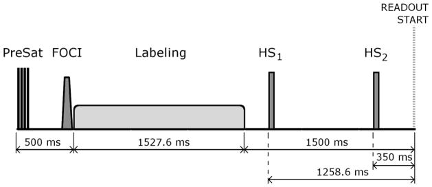
Background Suppression (BS) scheme implemented in the 3D single-shot imaging sequences, which consisted of 4 presaturation pulses, a slice-selective Frequency Offset Corrected Inversion (FOCI) pulse with C-shape, and two non-selective hyperbolic secant inversion pulses (HS1 and HS2) with inversion times optimized to suppress the static tissue signal to 10% of its original value. Also shown are the pCASL pulse and the readout start time.
The nominal resolution of all three sequences was kept constant at 4×4×6 mm3. The repetition time (TR) was 4 s. The readout parameters were selected as follows:
2D EPI: TR = 4000 ms, echo time (TE) = 18 ms, excitation flip angle = 90°, in-plane resolution = 4×4 mm2, matrix = 64×64, slice thickness = 6 mm, 16 slices with 1.5 mm gap acquired in ascending order, BW = 2790 Hz/px, FOV = 256×256 mm2, phase-encoding direction = anterior-posterior (A-P), total readout time (for all 16 slices) = 700 ms.
3D GRASE: TR/TE = 4000/29 ms, excitation flip angle = 90°, refocusing flip angle = 180°, resolution = 4×4×6 mm3, matrix = 64×57×11, 16 partitions in the slice-encoding direction with 12.5% oversampling acquired with a centric encoding scheme and slice partial Fourier (PF) = 5/8, BW = 2790 Hz/px, FOV = 256×224×96 mm3, in-plane phase-encoding direction = A-P, total readout time (for the entire 3D volume) = 330 ms.
3D FSE spiral: TR/TE = 4000/10 ms, excitation flip angle = 90°, refocusing flip angle = 160°, resolution = 4×4×6 mm3, matrix = 64×64×11, 16 nominal partitions with 12.5% oversampling acquired with a centric encoding scheme and slice PF = 5/8, 2 stacks of interleaved spirals, maximum slew rate = 120 mT/(m·ms), maximum gradient amplitude = 36 mT/m, FOV = 256×256×96 mm3, total readout time (for the entire volume) = 360 ms.
The spiral readout trajectory was generated numerically (King et al., 1995). The spiral calculation code was derived from Dr. Brian Hargreaves’ code (http://mrsrl.stanford.edu/~brian/vdspiral/). Gradient raster time and ADC sampling time were 10 and 2.5 us, respectively. FOV limit was applied along the radial direction. Spiral imaging data were reconstructed using the standard regridding method with a Kaiser-Bessel window kernel (Nuttall, 1981), and a Voronoi diagram to correct non-uniform sampling density. The Fastest Fourier Transform in the West (FFTW) package (Frigo, 2005) was used to transform the regridded data into the image space.
Scanning Protocol
The study was carried out on a 3-Tesla Siemens Trio (Siemens, Erlangen, Germany) using a 12-channel head array, and consisted of two consecutive sessions in which baseline and functional perfusion data were acquired, respectively.
At the beginning of the first session, an anatomical T1-weighed image of each subject was acquired with a MPRAGE sequence, with the following imaging parameters: TR/TE = 1620/3.09 ms, TI = 950 ms, flip angle = 15°, FOV = 192×256×160 mm3, resolution = 1 mm isotropic, matrix = 192×256×160, 160 axial slices, scan-time = 5.2 min.
Next, Phase Contrast (PC) velocity MRI was used to calculate total incoming CBF, as described in (Aslan et al., 2010), for the purpose of estimating a calibration factor needed for absolute CBF quantification from the pCASL data. The calibration factor represents the percentage of labeled blood spins that are present at sequence readout time. This value not only depends on the efficiency of the labeling pulse, which was identical for all sequences, but also on the BS scheme, since non-ideal inversion pulses employed to suppress the background signal interfere with the longitudinal magnetization created during labeling, decreasing its amplitude.
To this end, a Time-Of-Flight (TOF) angiogram was acquired to visualize the Internal Carotid Arteries (ICAs) and the Vertebral Arteries (VAs), for correctly positioning the PC velocity MRI slice.
Then, subjects underwent five scanning runs. During each run, baseline perfusion images were acquired with one of the five pCASL sequence variants, in pseudo-randomized order. Baseline perfusion was assessed with the acquisition of 100 scans (50 pairs of label-control images) while the subjects were resting with their eyes open. In the case of BS 3D sequences, 10 additional scans were acquired without BS to obtain control images necessary for CBF quantification.
The second session consisted again of five scanning runs, in which functional data were acquired with the different sequences, in pseudo-randomized order, during a sensory-motor activation paradigm. Each run had a total duration of 120 scans (60 pairs of label-control images), divided into 6 alternating task and rest blocks of 20-scan duration each. In the task blocks, subjects were presented with a black and white checkerboard flashing at a frequency of 10 Hz, and were asked to perform a fingertapping task with their right hand while looking at the center of the board. In the rest blocks, subjects were presented with a fixation cross and asked to remain still, with eyes open.
Data Processing
Data processing and statistical analysis were conducted using SPM (version 8, Wellcome Trust Center for Neuroimaging, University College London, UK) and custom scripts in Matlab (Mathworks, MA, USA). Raw label and control images were realigned and co-registered to the anatomical dataset, and then surround subtraction was applied to obtain perfusion-weighted images with minimal BOLD signal contamination (Aguirre et al., 2002; Wang et al., 2008). CBF maps were calculated from the perfusion-weighted images using the single-compartment model (Wang et al., 2005), where the control magnetization was computed from the average control images obtained without BS. A mean baseline perfusion image and CBF map were computed by averaging the 50 pairs acquired during the baseline scan.
The anatomical images were normalized to the Montreal Neurological Institute standard template brain and the resulting normalization parameters were used to normalize the CBF maps acquired during the task-related activation paradigm. Normalized CBF maps were spatially smoothed with a 3D Gaussian kernel of 8 mm Full-Width at Half-Maximum (FWHM), to perform group-level analyses. Anatomical grey matter (GM), white matter (WM) and whole-brain masks were created for each subject, to extract mean GM, WM and whole-brain CBF values. All masks were obtained from the segmented tissue maps generated upon individual T1-weighted image segmentation. To avoid partial volume effects, only the inner voxels located in deep GM/WM were kept for the calculation of GM/WM mean CBF values (van Gelderen et al., 2008). To avoid the inclusion of possible susceptibility related artifacts found in ventral slices, only slices superior to the corpus callosum were included.
Baseline Perfusion Analysis
The performance of the five modalities of pCASL during baseline measurements was characterized by evaluating the following parameters: PC-MRI derived calibration factor, temporal signal-to-noise ratio (SNR), spatial SNR, and GM-to-WM contrast ratio.
The calibration factor was computed as the ratio between the whole-brain mean pCASL CBF value to the total incoming CBF measured with PC velocity MRI, divided by the total intracranial mass (g) to be in units of mL/min/100g. Note that here the whole-brain mean pCASL CBF is the value calculated without taking into account the labeling efficiency and the effect of the BS pulses on the ASL signal. The total incoming CBF was estimated from the PC velocity MRI images by manually drawing masks of the ICAs and VAs of each subject in the magnitude images, and measuring the mean intensity inside each mask in the corresponding phase images. This value was then converted to cm/s, and multiplied by the area covered by the arteries (cm2) to have a final estimator of the incoming blood flow in cm3/s, i.e., mL/s. The total intracranial mass was then employed to convert the measure to units of mL/min/100g. The total intracranial mass was calculated from the total intracranial volume, assuming a brain density of 1.06 g/ml, based on the GM and WM segmented maps (Aslan et al., 2010). It is important to note that quantification of absolute CBF from pCASL data, after applying the calibration factor obtained for each sequence, will yield the same whole-brain mean CBF for all sequence variants, equal to the PC MRI derived mean CBF value.
Temporal SNR (tSNR) was computed as the mean of the whole-brain perfusion signal in the time series, divided by its standard deviation.
Three spatial SNR (sSNR) values were computed: the sSNR in the gray matter (sSNR-GM), the sSNR in the white matter (sSNR-WM) and the sSNR of the global perfusion signal (sSNR-Global). They were calculated as the ratio between the mean perfusion signal in the corresponding regions and the background noise level. The background noise level was estimated by manually drawing two spherical Regions-Of-Interest (ROI) of 10 mm radius, in regions well outside the brain, and calculating the standard deviation of the noise signal. The value obtained was corrected for averaging effects (Reeder, 2007). The GM-to-WM contrast ratio was estimated as the ratio between the mean CBF values measured within the two regions.
Statistical differences in these parameters among sequences were assessed by means of one-way repeated measures ANOVAs (RM-ANOVA) with factor sequence, and post-hoc comparisons were carried out using Bonferroni correction.
Functional Activation Analysis
The functional activation data were assessed for each sequence, first at the subject level, using the general linear model (Henson, 2004) by fitting the data into a block-design with two alternating conditions, rest and task. Individual contrast maps of the comparison between task and rest were obtained for each subject, and entered into a second level analysis for group level assessment. Group t-maps were calculated by means of a one-sample t-test and thresholded at p < 0.05 (family-wise error (FWE) corrected at cluster-level, cluster-defining threshold p = 0.001). Map-wise analysis at this corrected level of significance failed to identify activated areas in the maps obtained with the unsuppressed sequences. Thus, statistical significance was also assessed at an uncorrected threshold of p < 0.005.
Maximum voxel t-values were extracted at both the subject and group levels within two ROIs: an ROI located in the hand area of the left primary motor cortex (M1, Brodmann area (BA) 4), and an ROI in the primary visual cortex (V1, BA 17) (Figure 2). Within each ROI, the maximum t-values were identified in each sequence activation map. As the anatomical location of the hand motor area has been well established in the literature (Yousry et al., 1997), defined to have an inverted omega shape on the precentral gyrus, this shape was identified in every subject for the subject-level analysis, and in the left hemisphere of the MNI standard template for the group-level analysis, following the procedure in (Pimentel et al., 2011), and its center-of-gravity (COG) was calculated in order to estimate the distance between the voxel of maximum t-value within each M1 ROI and its corresponding anatomical M1 COG. At the subject level, percent CBF (% CBF) changes between task and rest conditions were also measured in M1 and V1, in spherical ROIs of 6 mm radius, centered at the voxels of maximum significance in the group maps. % CBF changes were calculated as the CBF increment observed within the sphere during the sensory-motor task compared to the rest period, relative to the CBF value during rest.
Figure 2.

(a) Left M1 (left BA 4) and (b) V1 (BA 17) masks employed to assess the maximum t-values obtained from the voxel-wise analysis of the task-related activation paradigm results, at subject and group levels. The BA 4 and BA 17 masks were extracted from the BA template provided with MRIcron.
The individual activation maps were finally entered in a one-way within-subject ANOVA with factor sequence to assess voxel-wise differences between sequences.
Simulation of the Point Spread Function in the Slice Encoding Direction
To assess the effect of signal decay in the slice encoding direction due to T2 on the effective resolution of the 3D sequences, the Point Spread Function (PSF) of both 3D GRASE and 3D FSE spiral readouts was computed by Fourier transforming the modulation transfer function, which was obtained by simulating the evolution of the signal during the readout time after the 90° excitation RF pulse, including stimulated and spin echoes, assuming blood T1 and T2 values of 1500 and 200 ms, respectively.
RESULTS
PC velocity MRI Results
The whole-brain mean CBF estimated for the ten subjects participating in the study from the PC velocity MRI data was 53.5 ± 7.9 mL/min/100g (mean ± SD across subjects). This result agrees well with values reported for this age range (for a review, see (Lassen, 1985)).
Baseline Perfusion Results
Representative perfusion and CBF maps from one subject acquired with the five tested sequences are displayed in Fig. 3. Table 1 summarizes the main parameters characterizing the performance of the five sequences. Unsuppressed 3D sequences demonstrated a 2-fold increase in sSNR compared to 2D EPI, whereas the calibration factor and the tSNR remained unchanged. GM-to-WM contrast decreased in the 3D sequences, particularly for the spiral readout, which showed the lowest contrast ratio among all sequences. The addition of BS to the 3D sequences yielded a 3-fold tSNR increase compared to the unsuppressed sequences. This tSNR increase was due to a dramatic reduction in the ASL signal variance. BS sequences presented a reduction in the calibration factor with respect to the unsuppressed ones, which reflected the attenuation of the ASL signal amplitude caused by the BS pulses. GM-to-WM contrast ratio was not affected by the use of BS.
Figure 3.

Representative perfusion (top) and CBF maps (bottom) from one subject acquired with the five tested sequences. The perfusion maps are displayed in coronal and axial orientation. The CBF scale bar indicates CBF units in mL/min/100g.
Table 1.
Comparison of baseline perfusion measurements obtained with 2D EPI, 3D GRASE, BS 3D GRASE, 3D FSE spiral and BS 3D FSE spiral. Values are given as mean ± standard deviation across subjects
| Sequence | 2D EPI | 3D GRASE | BS 3D GRASE | 3D FSE spiral | BS 3D FSE spiral | ||
|---|---|---|---|---|---|---|---|
| Whole-brain mean CBF (before calibration) | 46.4 ± 8.6 | 48.9 ± 11.4 | 38.1 ± 8.0 | 47.7 ± 9.5 | 38.4 ± 7.1 | ||
| Calibration factor (%) | 87.2 ± 13.2 | 92.2 + 19.4 | 71.2 ± 11.6 | 89.7 ± 15.6 | 72.2 ± 11.2 | ||
| Perfusion time- series | Mean | 6.7 ± 1.4 | 13.0 ± 3.4 | 10.1 ± 2.4 | 13.2 ± 2.8 | 10.6 ± 2.1 | |
| tSD | 2.1 ± 0.5 | 3.9 ± 0.8 | 1.1 ± 0.2 | 3.9 ± 0.7 | 1.0 ± 0.2 | ||
| tSNR | 3.5 ± 1.2 | 3.5 ± 1.5 | 10.1 ± 3.8 | 3.6 ± 1.2 | 10.2 ± 1.6 | ||
| SDnoise | 0.31 ± 0.04 | 0.28 ± 0.03 | 0.20 ± 0.01 | 0.28 ± 0.06 | 0.18 ± 0.04 | ||
| sSNR | Global | 2.9 ± 0.8 | 6.2 ± 2.0 | 6.7 ± 1.9 | 6.3 ± 1.4 | 7.8 ± 1.4 | |
| GM | 4.5 ± 1.2 | 9.1 ± 3.0 | 10.4 ± 2.7 | 10.2 ± 2.1 | 13.0 ± 2.2 | ||
| WM | 1.1 ± 0.5 | 2.8 ± 1.3 | 3.2 ± 1.2 | 6.3 ± 1.4 | 8.1 ± 1.6 | ||
| GM-WM CBF Contrast | 3.9 ± 1.1 | 3.1 ± 0.9 | 3.0 ± 0.6 | 1.8 ± 0.1 | 1.7 ± 0.1 | ||
tSD: temporal standard deviation; tSNR: temporal signal-to-noise ratio; SDnoise: background noise standard deviation; sSNR: spatial signal-to-noise ratio, corrected for averaging; GM: grey matter; WM: white matter; CBF: cerebral blood flow; EPI: echo-planar imaging; GRASE: gradient and spin-echo; FSE: fast spin-echo; BS: background suppression
The RM-ANOVAs performed over parameters calibration factor, tSNR, sSNR-Global, and GM-to-WM CBF contrast with factor sequence yielded statistically significant differences (p < 0.05, Bonferroni corrected), which further confirmed the previous observations. The following post-hoc pair-wise comparisons between sequences proved significant:
In the calibration factor, significant differences were found between sequences with BS (BS 3D GRASE and BS 3D FSE spiral) and sequences without BS (2D EPI, 3D GRASE and 3D FSE spiral).
Similarly, in the tSNR, significant differences were found between sequences with BS and sequences without BS.
In sSNR-Global, differences were significant between 3D sequences (with and without BS) and 2D EPI. BS 3D FSE spiral also showed a significant increase over BS 3D GRASE.
In the GM-to-WM contrast ratio, spiral readout yielded a significantly lower value than to 2D EPI and 3D GRASE.
Susceptibility induced off-resonance effects were observed in the orbito-frontal region in the perfusion maps, in the form of signal loss in the case of 2D EPI, and in the form of signal distortion in 3D GRASE (both with and without BS). In contrast, 3D FSE spiral perfusion maps showed better coverage in this region (See Figure 4 for a sample from a representative subject).
Figure 4.

Ventral slices of mean perfusion maps from a representative subject obtained with the five readout sequences. The arrows identify areas of distortion and signal loss. The intensity scale of each image was individually adjusted to improve visualization.
Functional Activation Results
Group task activation maps are shown in Figure 5, thresholded at p < 0.005 uncorrected (Figure 5a) and at p < 0.05 FWE cluster corrected (Figure 5b). Note that no significant clusters were obtained from the unsuppressed sequences (2D EPI, 3D GRASE and 3D FSE spiral) data after correction. In some of the uncorrected group maps, clusters of spurious activation could be observed in certain areas. Nevertheless, none of these clusters survived the cluster-level correction.
Figure 5.

Sensory-motor task group activation maps, superimposed on axial T1-weighted images, thresholded at (a) p < 0.005 uncorrected; (b) p < 0.05 FWE cluster-wise corrected (cluster-defining threshold p = 0.001). The color scale represents statistical significance (t) values.
Table 2 shows a summary of the maximum t-values extracted from the individual and group maps, for each of the sequences under test. At the subject level, unsuppressed 3D sequences yielded similar t-values compared to 2D EPI. When BS was employed, 3-fold higher t-values were obtained in V1 and M1 regions, as a result of the higher signal stability. At the group level, the maximum t-values obtained with the unsuppressed 3D sequences were again comparable to those of 2D EPI, however the cluster extent of the significant clusters was larger in the 3D sequences. BS also yielded higher t-values than the unsuppressed sequences at the group level, though 2D EPI values approached those of the BS 3D sequences in the M1 region.
Table 2.
Assessment of the task-related activation paradigm results at the subject and group levels. MNI coordinates (in mm) locate the maximum t-values within the bilateral V1 (BA 17) and left M1 (left BA 4) regions. Cluster-size is also given in units of voxels. In left M1, the distance from the voxel of maximum activation to the anatomically defined M1 region is reported. Values are expressed as mean ± SD across subjects
| Sequence | Type of analysis | Maximum t-value | Cluster - size (vox) | % CBF | MNI coordinates (mm)
|
Distance to M1 COG (mm) | |||
|---|---|---|---|---|---|---|---|---|---|
| X | Y | Z | |||||||
| LEFT V1 | 2D EPI | Subject | 3.4 ± 1.1 | −11.8 ± 6.4 | −94.2 ± 15.0 | 5.2 ± 7.1 | |||
|
| |||||||||
| Group | 3.7 | 9 | 19.4 ± 22.6 | −8.0 | −102.0 | 4.0 | |||
|
| |||||||||
| 3D GRASE | Subject | 2.5 ± 0.7 | −11.8 ± 5.8 | −97.2 ± 7.8 | 3.2 ± 7.5 | ||||
|
| |||||||||
| Group | 8.2 | 155 | 12.4 ± 5.6 | −12.0 | −98.0 | 6.0 | |||
|
| |||||||||
| BS 3D GRASE | Subject | 8.6 ± 2.4 | −12.2 ± 5.5 | −97.0 ± 5.8 | 3.6 ± 7.5 | ||||
|
| |||||||||
| Group | 20.2 | 7679 | 21.0 ± 5.5 | −4.0 | −88.0 | −6.0 | |||
|
| |||||||||
| 3D FSE spiral | Subject | 2.8 ± 1.3 | −10.0 ± 6.3 | −90.0 ± 12.9 | 4.8 ± 10.3 | ||||
|
| |||||||||
| Group | 3.4 | 351 | 16.1 ± 18.6 | −2.0 | −82.0 | 12.0 | |||
|
| |||||||||
| BS 3D FSE spiral | Subject | 9.4 ± 3.1 | −13.4 ± 5.2 | −96.0 ± 6.9 | 2.4 ± 8.4 | ||||
|
| |||||||||
| Group | 14.5 | 13025 | 23.1 ± 6.5 | −2.0 | −88.0 | −14.0 | |||
|
| |||||||||
| RIGHT V1 | 2D EPI | Subject | 2.8 ± 0.9 | 13.4 ± 6.7 | −90.6 ± 10.6 | 4.6 ± 6.5 | |||
|
| |||||||||
| Group | 9.9 | 62 | 27.8 ± 15.1 | 14.0 | −100.0 | 10.0 | |||
|
| |||||||||
| 3D GRASE | Subject | 2.3 ± 0.7 | 14.6 ± 7.1 | −92.6 ± 9.8 | 5.0 ± 9.1 | ||||
|
| |||||||||
| Group | 4.8 | 303 | 12.3 ± 9.0 | 16.0 | −96.0 | 8.0 | |||
|
| |||||||||
| BS 3D GRASE | Subject | 7.9 ± 2.1 | 12.2 ± 6.4 | −92.2 ± 7.6 | 6.6 ± 7.5 | ||||
|
| |||||||||
| Group | 15.7 | 7679 | 20.5 ± 6.1 | 2.0 | −84.0 | −8.0 | |||
|
| |||||||||
| 3D FSE spiral | Subject | 2.8 ± 1.5 | 13.2 ± 5.8 | −92.0 ± 9.3 | 5.6 ± 9.2 | ||||
|
| |||||||||
| Group | 3.9 | 351 | 17.7 ± 16.1 | 12.0 | −96.0 | 20.0 | |||
|
| |||||||||
| BS 3D FSE spiral | Subject | 8.8 ± 2.5 | 9.2 ± 5.8 | −91.0 ± 6.9 | 3.4 ± 11.7 | ||||
|
| |||||||||
| Group | 14.8 | 13025 | 21.5 ± 6.2 | 2.0 | −90.0 | −12.0 | |||
|
| |||||||||
| LEFT M1 | 2D EPI | Subject | 2.8 ± 0.9 | −37.8 ± 15.5 | −21.0 ± 8.5 | 62.4 ± 12.6 | 20.3 ± 13.1 | ||
|
| |||||||||
| Group | 8.8 | 129 | 31.3 ± 15.4 | −38.0 | −24.0 | 66.0 | 12.4 | ||
|
| |||||||||
| 3D GRASE | Subject | 2.8 ± 0.8 | −32.6 ± 18.0 | −22.8 ± 6.8 | 60.8 ± 9.3 | 18.3 ± 12.0 | |||
|
| |||||||||
| Group | 8.3 | 879 | 29.2 ± 13.4 | −40.0 | −20.0 | 62.0 | 10.2 | ||
|
| |||||||||
| BS 3D GRASE | Subject | 8.2 ± 2.3 | −38.2 ± 1.1 | −21.0 ± 3.9 | 60.0 ± 3.3 | 7.8 ± 4.3 | |||
|
| |||||||||
| Group | 10.3 | 3199 | 27.4 ± 10.9 | −36.0 | −20.0 | 60.0 | 7.3 | ||
|
| |||||||||
| 3D FSE spiral | Subject | 4.8 ± 2.6 | −37.0 ± 3.7 | −22.0 ± 4.0 | 58.0 ± 6.9 | 8.6 ± 2.9 | |||
|
| |||||||||
| Group | 5.1 | 567 | 17.5 ± 13.7 | −36.0 | −22.0 | 52.0 | 3.0 | ||
|
| |||||||||
| BS 3D FSE spiral | Subject | 10.2 ± 3.0 | −35.8 ± 3.0 | −21.2 ± 2.7 | 62.8 ± 8.4 | 10.4 ± 5.2 | |||
|
| |||||||||
| Group | 8.5 | 4675 | 21.1 ± 8.7 | −36.0 | −20.0 | 62.0 | 9.0 | ||
V1: Primary Visual Cortex; M1: Primary Motor Cortex; BA: Brodmann Area; % CBF: Percent Cerebral Blood Flow change, measured in a sphere of 6 mm radius, centered at the voxels of maximum significance in the group maps; EPI: echo-planar imaging; GRASE: gradient and spin-echo; FSE: fast spin-echo; BS: Background Suppression
Analysis at M1 region showed that 2D EPI maximum t-values were located more distant to the anatomically determined M1 COG, compared to the 3D sequences.
The % CBF increases measured at the M1 and V1 group maxima agree well with previous results in the literature (Aslan and Lu, 2010; Garraux et al., 2005; Tjandra et al., 2005). In general, larger % CBF changes were found for 2D EPI, in comparison with the 3D sequences.
Finally, the voxel-wise one-way within subject ANOVA yielded significant differences at a corrected p < 0.05 threshold. Post-hoc sequence comparisons showed that BS 3D FSE spiral presented significantly higher activation in V1 than 2D EPI (p < 0.05 FWE corrected for cluster extent).
Simulated PSF in the Slice Encoding Direction
The simulated PSFs of 3D GRASE and 3D FSE spiral in the slice-encoding direction are represented in Figure 6. The calculated FWHM of the 3D GRASE PSF was 1.38 voxels, with the PSF of 3D FSE spiral readout being 3.4% wider.
Figure 6.

Simulated point spread functions (PSFs) in the slice encoding direction for 3D GRASE (solid line) and 3D FSE spiral (dashed line) readouts. The dashed horizontal line indicates the location of the PSF half maximum amplitude.
DISCUSSION
The effect of readout choice in pCASL perfusion MRI sequences was assessed in this work. To this end, five sequence variants were compared in a group of ten young healthy volunteers, both during a baseline perfusion measurement and during a functional study with a sensory-motor activation paradigm. Implementations of 2D EPI, 3D GRASE and 3D FSE spiral, with the same repetition time, resolution and identical pCASL pulse were compared. In 2D readouts each slice has a different acquisition time, which complicates the use of BS because the level of signal suppression will vary from slice to slice. Therefore, in this work we chose to assess the impact of BS only with the 3D sequence modalities.
The sequences were selected amongst the most commonly employed in the literature. In 2D EPI, each slice is individually excited. This sequence has been traditionally chosen for ASL measurements due to its high sensitivity and temporal resolution, despite being prone to off-resonance effects arising from magnetic susceptibility variations (e.g. tissue-air interfaces). On the other hand, 3D GRASE and 3D FSE spiral are fast spin echo based sequences, thus suffering only from T2 decay in the slice-encoding direction, since the refocusing pulses rephase the spin dephasing caused by inhomogeneities in the B0 field at every spin-echo time. Note that, as implemented here, only the 3D GRASE sequence takes full advantage of this effect, since it is the only one in which the center of each k-space plane is sampled at precisely the spin echo time, within a Cartesian in-plane trajectory. On the other hand, the spiral readout provides minimum TE, since the center of k-space is sampled at the beginning of the readout. In addition, spiral readouts generally offer more flexibility in the trajectory design, such as variable density sampling and the use of multiple stacks of interleaved spirals, which shortens the sampling time between refocusing pulses, and thus decreases the sensitivity to susceptibility variations. Another advantage of the spiral readout design is that the center of k-space is oversampled, which increases robustness against motion artifacts, with the inherent refocusing of motion and flow-induced phase errors, due to the shape of the gradients (Ahn et al., 1986; Delattre et al., 2010; King, 2004; Liao et al., 1997).
Baseline Perfusion Measurements
The calibration factor of pCASL when no BS was applied was found to be 87–92%. This parameter in the absence of BS is equivalent to the labeling efficiency. The calculated values are in excellent agreement with the results in the literature (Aslan et al., 2010; Dai et al., 2008). Moreover, there was no difference between the calibration factor obtained for 2D EPI and the 3D sequences without BS. This implies that the longer effective post-labeling delays in 2D EPI particularly for the upper slices, do not affect the CBF quantification, probably due to the long post-labeling delay of 1.5 s employed in the acquisitions, which is longer than arrival times measured in healthy young adults, for all vascular territories (Chen et al., 2012; Wang et al., 2003). The BS scheme was designed to suppress the static tissue signal to 10% of its original value. It is known that the use of BS also produces an attenuation of the ASL signal, here measured as a reduction in the calibration factor of the BS 3D sequences. The observed calibration factor when BS was applied was 71–72%, which implies that each of the non-selective inversion pulses had an inversion efficiency of 90%. This value matches the results obtained for optimized in-vivo BS schemes (Garcia et al., 2005).
Spatial SNR increased 2-fold in the unsuppressed 3D readouts, compared to 2D EPI. This increase reflects the higher SNR efficiency of 3D acquisitions (since the signal from the whole volume is sampled for every excitation) and the larger effective voxel size (in slice direction) (as shown by the PSF calculations).
The sSNR measurements increased slightly in the perfusion maps acquired with BS 3D readouts, as compared to unsuppressed 3D. This result is most likely an artifact, since with BS the perfusion signal is attenuated and therefore the perfusion map sSNR should decrease, when measured relative to background noise, which should not be affected by BS (Robson et al., 2009). However, the noise standard deviation appears to be reduced by BS (see Table 1). This most likely means that although the background ROIs were placed in areas apparently devoid of signal, the noise measurements must be affected by signal artifacts extending to background areas. These artifacts (ghost images in the phase encoding direction in the 3D GRASE images or reconstruction artifacts in the 3D FSE spiral images) are probably attenuated by BS, thus causing an apparent reduction of the noise and an artificial increase in the sSNR.
In spite of the attenuation of the ASL signal caused by BS, there was a 3-fold increase in the temporal SNR of BS sequences, compared to the unsuppressed ones. In contrast, no differences were observed between 2D and 3D readout sequences without BS, despite recent work (Nielsen and Hernandez-Garcia, 2012) suggesting that tSNR increases in an optimized 3D sequence with respect to 2D. However, in the data presented here, although the mean of the ASL signal increased for the 3D acquisitions, its temporal standard deviation increased proportionally and decreased only when BS was employed (see Table 1). BS data showed reduced variance due to the higher temporal stability caused by the suppression of physiological noise, which translated into higher tSNR (Gunther et al., 2005; Ye et al., 2000).
In both tSNR and sSNR measures, a trend was observed showing slightly higher SNR values for the spiral readout. The shorter TE of the spiral readout and some of its intrinsic advantages, such as its relative insensitivity to movement and flow artifacts (Ahn et al., 1986; Delattre et al., 2010; King, 2004; Liao et al., 1997), may be contributing to achieve higher SNR values, but this could also be due to the in-plane blurring observed in the spiral images.
The GM-to-WM CBF contrast values measured with all the sequences were in the range of the results found in the literature, although there is a high variability in this measure among the reported values (Fernandez-Seara et al., 2005; Gunther et al., 2005; Wang et al., 2005; Xu et al., 2010). A higher GM-to-WM CBF contrast was obtained with the 2D EPI sequence, compared to the 3D sequences, consistent with previous reports (Fernandez-Seara et al., 2005). The decrease in contrast observed with the 3D sequences was likely due to more severe partial volume effects, generated by the additional smoothing in the slice-encoding direction that appears due to T2 decay. BS demonstrated no effect on this measure, as contrast did not vary in either 3D GRASE or 3D FSE spiral when adding BS.
The 3D FSE spiral sequences showed lower GM-to-WM CBF contrast, compared to 3D GRASE. Since both modalities had comparable total readout times (330 ms for 3D GRASE and 360 ms for 3D FSE spiral), no significant effect due to additional T2 decay was expected in the spiral readout. A difference between the two readout designs was that the spiral readout comprised twice the number of refocusing pulses, due to the use of two stacks of interleaved spirals in every partition, and because of that the refocusing flip angle of these pulses was decreased to 160° due to SAR limitations. To evaluate the effect of this difference, we compared the PSFs of both FSE spiral and GRASE readouts in the slice-encoding direction (Figure 6). The difference between PSF widths was negligible (spiral’s PSF FWHM was less than 3.5% wider), hence, the influence of the slice-encoding scheme was ruled out as a possible source of additional smoothing.
Other sources of blurring in the spiral sequence could arise from deviations between the theoretical and the real gradient waveforms (Delattre et al., 2010; King, 2004), which can lead to additional blurring in the reconstruction step, due to the use of inexact k-space trajectories. Likewise, off-resonance effects due to B0 field inhomogeneities or magnetic susceptibility changes manifest themselves in spiral sequences as blurring, their effect being more severe in sequences with long readout times (Delattre et al., 2010; King, 2004). Multi-shot spiral acquisitions are expected to alleviate blurring by reducing the total readout time and consequently the accumulated phase error, though these sequences are less versatile in functional activation studies because of their reduced temporal resolution, as several TRs are needed for the acquisition of a single image. However, certain activation or pharmacological paradigms are suitable for monitoring with reduced temporal resolution and for such studies multi-shot approaches would be attractive.
In future work, implementation of real-time measurement of spiral gradient waveforms prior to image acquisition as well as B0 field inhomogeneity correction should help reducing possible sources of blurring (Cheng et al., 2011; Delattre et al., 2010; Tan and Meyer, 2009).
Perfusion maps acquired with the 2D EPI sequence showed signal losses in the orbito-frontal cortex, attributable to magnetic susceptibility variations (Cho and Ro, 1992). In 3D GRASE there was no signal loss in this region, but image distortions were observed due to displacement of the signal in the phase-encoding direction caused by the susceptibility background gradients (Fernandez-Seara et al., 2005). In contrast, 3D FSE spiral showed no signal loss or distortion about the orbito-frontal region. Since increased susceptibility differences have the effect of shortening T2*, it is likely that the shorter TE of the spiral readout contributes to making this sequence more robust against these off-resonance effects.
Functional Activation Measurements
The functional experiments showed the expected areas of activation at the group level in contralateral primary motor cortex (M1, hand area) and bilateral primary visual cortex (V1). These results coincide well with the regions reported by previous studies with similar activation paradigms (Aguirre et al., 2002; Aslan and Lu, 2010; Buxton et al., 1998; Tjandra et al., 2005; Yang et al., 1998; Ye et al., 1997). In addition, BS 3D sequences showed activation in the supplementary motor area (SMA), pre-SMA, putamen and thalamus, which are known to be involved in the execution of voluntary movements, although only the SMA cluster of BS 3D FSE spiral survived correction.
Two main effects were observed when analyzing the statistical significance of the activation maps. At the individual level, the use of BS 3D readouts increased the t-values in both left M1 and bilateral V1, by a factor of 3, with respect to the unsuppressed sequences. This is likely a consequence of the increased tSNR, i.e. reduced physiological noise, realized by BS, as has been previously observed employing a different functional task (Ye et al., 2000). This increase in within-subject statistical power was observed in spite of a reduction in the effect size (% CBF change) measured with the 3D readouts. The reduction in effect size is probably attributable to the more severe partial volume effects in the 3D sequences, reflected as well in the lower GM-to-WM contrast ratio of the perfusion maps.
At the group level, the differences between sequences were reduced, particularly in the M1 region. Although the group activation maps obtained with the unsuppressed 2D EPI did not survive correction for multiple comparisons, the maximum uncorrected t-values increased considerably compared to the t-values seen at the subject level (see Table 2). This is consistent with prior observations obtained using unsuppressed 2D EPI ASL indicating that group level activation with ASL may be more robust that individual level activation, presumably due to conservation of task-induced CBF changes (Aguirre et al., 2002; Tjandra et al., 2005). This effect was not as pronounced in the BS 3D ASL sequences, most probably due to their already high sensitivity for task activation at the individual subject level resulting from increased tSNR, though t-values also increased between individual and group levels for BS 3D ASL. Taken together, these findings suggest that the sensitivity benefits of the 3D BS sequences, while dramatic at the individual level, can be offset at the group level by consistent changes in CBF in response to task.
While unsuppressed 3D sequences presented similar significance values to those of 2D EPI, the size of activated clusters in these maps was larger, which could be a consequence of the increased effective voxel size.
In summary, at the subject level, the use of BS 3D readouts resulted in enhanced sensitivity due to increased tSNR, in spite of the effect size reduction. Improved sensitivity at the subject level could be particularly important for clinical applications of ASL fMRI or for studies focusing on individual differences in activation. Further improvements in 3D imaging, such as accelerated acquisitions or improved k-space trajectories should allow approaching or exceeding the resolution of 2D EPI, thus eliminating the reduction in effect size and allowing the full realization of the benefits of combining 3D readouts with BS.
In conclusion, the results of this study demonstrate that the combination of 3D single-shot imaging sequences with BS techniques considerably improves the performance of pCASL sequences in baseline and functional activation studies, with the major contribution to the increase in sensitivity for functional studies coming from the use of BS.
Highlights.
3D pCASL sequences increased perfusion spatial SNR by a factor of 2
The addition of BS to 3D readouts increased perfusion temporal SNR by a factor of 3
2D EPI showed higher GM-to-WM CBF contrast ratio
Statistical power to detect functional activation was higher in 3D BS sequences
3D BS single-shot sequences appear as the preferable readout choice in pCASL fMRI
Acknowledgments
We are thankful to Dr. David Alsop for his help with the implementation of the 3D FSE spiral sequence and BS optimization. We also thank Drs. Josef Pfeuffer and Tiejun Zhao from Siemens for their help with the spiral readout sequence and online reconstruction programming. We thank Drs. David Feinberg and Matthias Guenther for sharing the original 3D GRASE source code. This work was supported by the Spanish Ministry of Science and Innovation (grants SAF2008-00678 and RYC-2010-07161) and the National Institutes of Health (grants R01MH080729 and RR02305).
Footnotes
Publisher's Disclaimer: This is a PDF file of an unedited manuscript that has been accepted for publication. As a service to our customers we are providing this early version of the manuscript. The manuscript will undergo copyediting, typesetting, and review of the resulting proof before it is published in its final citable form. Please note that during the production process errors may be discovered which could affect the content, and all legal disclaimers that apply to the journal pertain.
References
- Aguirre GK, Detre JA, Zarahn E, Alsop DC. Experimental design and the relative sensitivity of BOLD and perfusion fMRI. Neuroimage. 2002;15:488–500. doi: 10.1006/nimg.2001.0990. [DOI] [PubMed] [Google Scholar]
- Ahn CB, Kim JH, Cho ZH. High-speed spiral-scan echo planar NMR imaging-I. IEEE Trans Med Imaging. 1986;5:2–7. doi: 10.1109/TMI.1986.4307732. [DOI] [PubMed] [Google Scholar]
- Aslan S, Lu H. On the sensitivity of ASL MRI in detecting regional differences in cerebral blood flow. Magn Reson Imaging. 2010;28:928–935. doi: 10.1016/j.mri.2010.03.037. [DOI] [PMC free article] [PubMed] [Google Scholar]
- Aslan S, Xu F, Wang PL, Uh J, Yezhuvath US, van Osch M, Lu H. Estimation of labeling efficiency in pseudocontinuous arterial spin labeling. Magn Reson Med. 2010;63:765–771. doi: 10.1002/mrm.22245. [DOI] [PMC free article] [PubMed] [Google Scholar]
- Buxton RB, Frank LR, Wong EC, Siewert B, Warach S, Edelman RR. A general kinetic model for quantitative perfusion imaging with arterial spin labeling. Magn Reson Med. 1998;40:383–396. doi: 10.1002/mrm.1910400308. [DOI] [PubMed] [Google Scholar]
- Chen Y, Wang DJ, Detre JA. Comparison of arterial transit times estimated using arterial spin labeling. MAGMA. 2012;25:135–144. doi: 10.1007/s10334-011-0276-5. [DOI] [PubMed] [Google Scholar]
- Cheng JY, Santos JM, Pauly JM. Fast concomitant gradient field and field inhomogeneity correction for spiral cardiac imaging. Magn Reson Med. 2011;66:390–401. doi: 10.1002/mrm.22802. [DOI] [PMC free article] [PubMed] [Google Scholar]
- Cho ZH, Ro YM. Reduction of susceptibility artifact in gradient-echo imaging. Magn Reson Med. 1992;23:193–200. doi: 10.1002/mrm.1910230120. [DOI] [PubMed] [Google Scholar]
- Dai W, Garcia D, de Bazelaire C, Alsop DC. Continuous flow-driven inversion for arterial spin labeling using pulsed radio frequency and gradient fields. Magn Reson Med. 2008;60:1488–1497. doi: 10.1002/mrm.21790. [DOI] [PMC free article] [PubMed] [Google Scholar]
- Delattre BM, Heidemann RM, Crowe LA, Vallee JP, Hyacinthe JN. Spiral demystified. Magn Reson Imaging. 2010;28:862–881. doi: 10.1016/j.mri.2010.03.036. [DOI] [PubMed] [Google Scholar]
- Detre JA, Leigh JS, Williams DS, Koretsky AP. Perfusion imaging. Magn Reson Med. 1992;23:37–45. doi: 10.1002/mrm.1910230106. [DOI] [PubMed] [Google Scholar]
- Detre JA, Rao H, Wang DJ, Chen YF, Wang Z. Applications of arterial spin labeled MRI in the brain. J Magn Reson Imaging. 2012;35:1026–1037. doi: 10.1002/jmri.23581. [DOI] [PMC free article] [PubMed] [Google Scholar]
- Duhamel G, Alsop DC. Single-shot susceptibility insensitive whole brain 3D fMRI with ASL. Proceedings of the 12th Annual Meeting of ISMRM; Kyoto. 2004. p. 518. [Google Scholar]
- Fernandez-Seara MA, Edlow BL, Hoang A, Wang J, Feinberg DA, Detre JA. Minimizing acquisition time of arterial spin labeling at 3T. Magn Reson Med. 2008;59:1467–1471. doi: 10.1002/mrm.21633. [DOI] [PubMed] [Google Scholar]
- Fernandez-Seara MA, Wang Z, Wang J, Rao HY, Guenther M, Feinberg DA, Detre JA. Continuous arterial spin labeling perfusion measurements using single shot 3D GRASE at 3 T. Magn Reson Med. 2005;54:1241–1247. doi: 10.1002/mrm.20674. [DOI] [PubMed] [Google Scholar]
- Frigo M, Johnson SG. The design and implementation of FFTW3. Proc IEEE. 2005;93:216–231. [Google Scholar]
- Gai ND, Talagala SL, Butman JA. Whole-brain cerebral blood flow mapping using 3D echo planar imaging and pulsed arterial tagging. J Magn Reson Imaging. 2011;33:287–295. doi: 10.1002/jmri.22437. [DOI] [PMC free article] [PubMed] [Google Scholar]
- Garcia DM, Duhamel G, Alsop DC. Efficiency of inversion pulses for background suppressed arterial spin labeling. Magn Reson Med. 2005;54:366–372. doi: 10.1002/mrm.20556. [DOI] [PubMed] [Google Scholar]
- Garraux G, Hallett M, Talagala SL. CASL fMRI of subcortico-cortical perfusion changes during memory-guided finger sequences. Neuroimage. 2005;25:122–132. doi: 10.1016/j.neuroimage.2004.11.004. [DOI] [PubMed] [Google Scholar]
- Gunther M, Oshio K, Feinberg DA. Single-shot 3D imaging techniques improve arterial spin labeling perfusion measurements. Magn Reson Med. 2005;54:491–498. doi: 10.1002/mrm.20580. [DOI] [PubMed] [Google Scholar]
- Henson RNA. Analysis of fMRI time series. In: Frackowiak RSJ, Friston KJ, Frith C, Dolan R, Price CJ, Zeki S, Ashburner J, Penny WD, editors. Human Brain Function. Academic Press; London: 2004. pp. 793–822. [Google Scholar]
- Huppert TJ, Hoge RD, Diamond SG, Franceschini MA, Boas DA. A temporal comparison of BOLD, ASL, and NIRS hemodynamic responses to motor stimuli in adult humans. Neuroimage. 2006;29:368–382. doi: 10.1016/j.neuroimage.2005.08.065. [DOI] [PMC free article] [PubMed] [Google Scholar]
- King KF. Spiral. In: Bernstein MA, King K, Zhou X, editors. Handbook of MRI pulse sequences. Elsevier Academic Press; London: 2004. pp. 928–954. [Google Scholar]
- King KF, Foo TK, Crawford CR. Optimized gradient waveforms for spiral scanning. Magn Reson Med. 1995;34:156–160. doi: 10.1002/mrm.1910340205. [DOI] [PubMed] [Google Scholar]
- Lassen NA. Normal average value of cerebral blood flow in younger adults is 50 ml/100 g/min. J Cereb Blood Flow Metab. 1985;5:347–349. doi: 10.1038/jcbfm.1985.48. [DOI] [PubMed] [Google Scholar]
- Liao JR, Pauly JM, Brosnan TJ, Pelc NJ. Reduction of motion artifacts in cine MRI using variable-density spiral trajectories. Magn Reson Med. 1997;37:569–575. doi: 10.1002/mrm.1910370416. [DOI] [PubMed] [Google Scholar]
- Maldjian JA, Laurienti PJ, Burdette JH. Precentral gyrus discrepancy in electronic versions of the Talairach atlas. Neuroimage. 2004;21:450–455. doi: 10.1016/j.neuroimage.2003.09.032. [DOI] [PubMed] [Google Scholar]
- Maldjian JA, Laurienti PJ, Kraft RA, Burdette JH. An automated method for neuroanatomic and cytoarchitectonic atlas-based interrogation of fMRI data sets. Neuroimage. 2003;19:1233–1239. doi: 10.1016/s1053-8119(03)00169-1. [DOI] [PubMed] [Google Scholar]
- Nielsen JF, Hernandez-Garcia L. Functional perfusion imaging using pseudocontinuous arterial spin labeling with low-flip-angle segmented 3D spiral readouts. Magn Reson Med. 2012 doi: 10.1002/mrm.24261. [DOI] [PubMed] [Google Scholar]
- Nuttall AH. Some windows with very good sidelobe behavior. IEEE Trans Acoust Speech Signal Processing. 1981;29:84–91. [Google Scholar]
- Pimentel MA, Vilela P, Sousa I, Figueiredo P. Localization of the hand motor area by arterial spin labeling and blood oxygen level-dependent functional magnetic resonance imaging. Hum Brain Mapp. 2011 doi: 10.1002/hbm.21418. [DOI] [PMC free article] [PubMed] [Google Scholar]
- Raichle ME. Behind the scenes of functional brain imaging: a historical and physiological perspective. Proc Natl Acad Sci U S A. 1998;95:765–772. doi: 10.1073/pnas.95.3.765. [DOI] [PMC free article] [PubMed] [Google Scholar]
- Reeder SB. Measurement of signal-to-noise ratio and parallel imaging. In: Schoenber SO, Dietrich O, Reiser MF, editors. Parallel Imaging in Clinical MR Applications. Springer; Heidelberg: 2007. pp. 49–61. [Google Scholar]
- Robson PM, Madhuranthakam AJ, Dai W, Pedrosa I, Rofsky NM, Alsop DC. Strategies for reducing respiratory motion artifacts in renal perfusion imaging with arterial spin labeling. Mag Reson Med. 2009;61:1374–1387. doi: 10.1002/mrm.21960. [DOI] [PMC free article] [PubMed] [Google Scholar]
- Silva AC, Lee SP, Iadecola C, Kim SG. Early temporal characteristics of cerebral blood flow and deoxyhemoglobin changes during somatosensory stimulation. J Cereb Blood Flow Metab. 2000;20:201–206. doi: 10.1097/00004647-200001000-00025. [DOI] [PubMed] [Google Scholar]
- Tan H, Meyer CH. Estimation of k-space trajectories in spiral MRI. Magn Reson Med. 2009;61:1396–1404. doi: 10.1002/mrm.21813. [DOI] [PMC free article] [PubMed] [Google Scholar]
- Tjandra T, Brooks JC, Figueiredo P, Wise R, Matthews PM, Tracey I. Quantitative assessment of the reproducibility of functional activation measured with BOLD and MR perfusion imaging: implications for clinical trial design. Neuroimage. 2005;27:393–401. doi: 10.1016/j.neuroimage.2005.04.021. [DOI] [PubMed] [Google Scholar]
- Tzourio-Mazoyer N, Landeau B, Papathanassiou D, Crivello F, Etard O, Delcroix N, Mazoyer B, Joliot M. Automated anatomical labeling of activations in SPM using a macroscopic anatomical parcellation of the MNI MRI single-subject brain. Neuroimage. 2002;15:273–289. doi: 10.1006/nimg.2001.0978. [DOI] [PubMed] [Google Scholar]
- van Gelderen P, de Zwart JA, Duyn JH. Pittfalls of MRI measurement of white matter perfusion based on arterial spin labeling. Magn Reson Med. 2008;59:788–795. doi: 10.1002/mrm.21515. [DOI] [PMC free article] [PubMed] [Google Scholar]
- Wang J, Aguirre GK, Kimberg DY, Roc AC, Li L, Detre JA. Arterial spin labeling perfusion fMRI with very low task frequency. Magn Reson Med. 2003;49:796–802. doi: 10.1002/mrm.10437. [DOI] [PubMed] [Google Scholar]
- Wang J, Zhang Y, Wolf RL, Roc AC, Alsop DC, Detre JA. Amplitude-modulated continuous arterial spin-labeling 3.0-T perfusion MR imaging with a single coil: feasibility study. Radiology. 2005;235:218–228. doi: 10.1148/radiol.2351031663. [DOI] [PubMed] [Google Scholar]
- Wang Z, Aguirre GK, Rao H, Wang J, Fernandez-Seara MA, Childress AR, Detre JA. Empirical optimization of ASL data analysis using an ASL data processing toolbox: ASLtbx. Magn Reson Imaging. 2008;26:261–269. doi: 10.1016/j.mri.2007.07.003. [DOI] [PMC free article] [PubMed] [Google Scholar]
- Williams DS, Detre JA, Leigh JS, Koretsky AP. Magnetic resonance imaging of perfusion using spin inversion of arterial water. Proc Natl Acad Sci U S A. 1992;89:212–216. doi: 10.1073/pnas.89.1.212. [DOI] [PMC free article] [PubMed] [Google Scholar]
- Wu WC, Edlow BL, Elliot MA, Wang J, Detre JA. Physiological modulations in arterial spin labeling perfusion magnetic resonance imaging. IEEE Trans Med Imaging. 2009;28:703–709. doi: 10.1109/TMI.2008.2012020. [DOI] [PubMed] [Google Scholar]
- Wu WC, Fernandez-Seara M, Detre JA, Wehrli FW, Wang J. A theoretical and experimental investigation of the tagging efficiency of pseudocontinuous arterial spin labeling. Magn Reson Med. 2007;58:1020–1027. doi: 10.1002/mrm.21403. [DOI] [PubMed] [Google Scholar]
- Xu G, Rowley HA, Wu G, Alsop DC, Shankaranarayanan A, Dowling M, Christian BT, Oakes TR, Johnson SC. Reliability and precision of pseudo-continuous arterial spin labeling perfusion MRI on 3.0 T and comparison with 15O-water PET in elderly subjects at risk for Alzheimer’s disease. NMR Biomed. 2010;23:286–293. doi: 10.1002/nbm.1462. [DOI] [PMC free article] [PubMed] [Google Scholar]
- Yang Y, Frank JA, Hou L, Ye FQ, McLaughlin AC, Duyn JH. Multislice imaging of quantitative cerebral perfusion with pulsed arterial spin labeling. Magn Reson Med. 1998;39:825–832. doi: 10.1002/mrm.1910390520. [DOI] [PubMed] [Google Scholar]
- Ye FQ, Frank JA, Weinberger DR, McLaughlin AC. Noise reduction in 3D perfusion imaging by attenuating the static signal in arterial spin tagging (ASSIST) Magn Reson Med. 2000;44:92–100. doi: 10.1002/1522-2594(200007)44:1<92::aid-mrm14>3.0.co;2-m. [DOI] [PubMed] [Google Scholar]
- Ye FQ, Smith AM, Yang Y, Duyn J, Mattay VS, Ruttimann UE, Frank JA, Weinberger DR, McLaughlin AC. Quantitation of regional cerebral blood flow increases during motor activation: a steady-state arterial spin tagging study. Neuroimage. 1997;6:104–112. doi: 10.1006/nimg.1997.0282. [DOI] [PubMed] [Google Scholar]
- Yousry TA, Schmid UD, Alkadhi H, Schmidt D, Peraud A, Buettner A, Winkler P. Localization of the motor hand area to a knob on the precentral gyrus. A new landmark. Brain. 1997;120(Pt 1):141–157. doi: 10.1093/brain/120.1.141. [DOI] [PubMed] [Google Scholar]