Abstract
In this paper we have coupled the CMAQ and ADMS air quality models to predict hourly concentrations of NOX, NO2 and O3 for London at a spatial scale of 20 m × 20 m. Model evaluation has demonstrated reasonable agreement with measurements from 80 monitoring sites in London. For NO2 the model evaluation statistics gave 73% of the hourly concentrations within a factor of two of observations, a mean bias of −4.7 ppb and normalised mean bias of −0.17, a RMSE value of 17.7 and an r value of 0.58. The equivalent results for O3 were 61% (FAC2), 2.8 ppb (MB), 0.15 (NMB), 12.1 (RMSE) and 0.64 (r). Analysis of the errors in the model predictions by hour of the week showed the need for improvements in predicting the magnitude of road transport related NOX emissions as well as the hourly emissions scaling in the model. These findings are consistent with recent evidence of UK road transport NOX emissions, reported elsewhere. The predictions of wind speed using the WRF model also influenced the model results and contributed to the daytime over prediction of NOX concentrations at the central London background site at Kensington and Chelsea. An investigation of the use of a simple NO–NO2–O3 chemistry scheme showed good performance close to road sources, and this is also consistent with previous studies. The coupling of the two models raises an issue of emissions double counting. Here, we have put forward a pragmatic solution to this problem with the result that a median double counting error of 0.42% exists across 39 roadside sites in London. Finally, whilst the model can be improved, the current results show promise and demonstrate that the use of a combination of regional scale and local scale models can provide a practical modelling tool for policy development at intergovernmental, national and local authority level, as well as for use in epidemiological studies.
Keywords: Road source modelling, CMAQ, Air quality, Model evaluation, London
Highlights
► We coupled the CMAQ and ADMS air quality models. ► We predicted hourly NOX, NO2 and O3 in London at 20 m × 20 m. ► Model evaluation has demonstrated reasonable agreement with 80 monitoring sites in London. ► Improvements are required in predicting the magnitude of road transport NOX emissions. ► The combination of regional and local scale models is a practical modelling tool.
1. Introduction
Air quality models are important tools in providing evidence of the impact on air quality of policy options at both regional and national scale under obligations to the National Emission Ceilings Directive (NEDC, 2001) and the Gothenburg Protocol (UNECE, 1999), and at city scale, to implement plans such as the Mayors Air Quality Strategy (GLA, 2010b) in London and numerous Low Emission Zones across Europe (http://www.lowemissionzones.eu/). In the UK concerns are focused on meeting NO2, PM10 and PM2.5 EU limit values (EC, 2008), on the impacts of short term climate forcing and on the impacts on sensitive ecosystems and crops. However, increasingly models are also being used as a source of human exposure information for epidemiological studies (Maheswaran et al., 2010; Tonne et al., 2010) and health impact assessments (e.g., Georgopoulos et al., 2005; Isakov et al., 2009; Woodcock et al., 2009). Epidemiological studies, which look cross-sectionally at health outcomes, require models to provide annual mean concentrations at fine spatial scales (post/zip code areas), but are increasingly required to elucidate a combination of spatio-temporal influences placing further demands on a model's temporal resolution. Finally, there is a need to take account of space-time-activity data (Ashmore, 2005) in exposure assessments both for policy development and to reflect the dose from pollutants that have a range of toxicity (such as PM) (Kelly et al., 2011) or of mixtures of pollutants (Molitor et al., 2011).
In an attempt to meet these demands in a large urban area, we describe the coupling of the Community Multiscale Air Quality (CMAQ) modelling system (Byun and Ching, 1999) and the Atmospheric Dispersion Modelling System (ADMS) Roads model (CERC, 2006). We provide details of the models performance in predicting hourly NOX–NO2–O3 concentrations over a detailed (20 m × 20 m) grid in London in 2006. The results for a similar run in 2008 are also provided in support of the 2006 evaluation and have been reported elsewhere (Carslaw, 2011).
2. Methods
2.1. CMAQ-urban COULPING
The regional scale (CMAQ) and local scale (ADMS) dispersion models have been coupled to create a model system (CMAQ-urban). In Section 2.2 details are given of the Weather Research and Forecasting (WRF) setup, in Section 2.3 details are given of the CMAQ setup, in Section 2.4 details are given of the ADMS setup and in Section 2.5 details are given of the outputs of CMAQ-urban.
2.2. WRF setup details
The WRF model v3.1 (Skamrock et al., 2008) was setup using 23 vertical layers with 7 layers under 800 m and the top layer ∼15 km above the ground. Four horizontal nesting levels were used, downscaling from 81 km grids over Europe to 27 km over the UK and Ireland, 9 km over the UK and 3 km over London. Initial and boundary (IC/BC) conditions were taken from the GFS model at 1 × 1° (http://www.esrl.noaa.gov/psd/data/reanalysis/reanalysis.shtml). Other physics settings within WRF included use of the Rapid Radiation Transfer Model (RRTM) radiation scheme (Mlawer et al., 1997), the Kain–Fritsch (new Eta) microphysics scheme (Kain, 2004), the Yonsei University (YSU) planetary boundary layer scheme (Hong et al., 2006), the Monin–Obukhov surface scheme (Skamrock et al., 2008) and the National Ocean and Atmospheric Administration (NOAA) land surface scheme (Chen and Dudhia, 2001). Observational nudging of wind speed, temperature and relative humidity was used in the WRF model with a nudging strength of 6 × 10⁻⁴ and radius of influence of 200 km. In urban areas urban land cover and Z0 values of 0.8 m were used. No anthropogenic heat from buildings or road transport was included in the WRF model.
2.3. CMAQ setup details
The CMAQ v4.6 model was setup using the same vertical and horizontal grid structure as for WRF. Atmospheric chemistry was simulated using the CB 05 chemical mechanism (Yarwood et al., 2005) and initial and boundary conditions, included as monthly means, from the UK Meteorological Office chemistry-transport model, STOCHEM (Derwent pers. comm.), which provided 14 pollutant species including CO, NH3, NOX, O3, HNO3 and VOC's. Anthropogenic and natural emissions were derived from the European Monitoring and Evaluation Programme (EMEP, http://www.ceip.at/), the European Pollutant Release and Transfer Register (EPETR), the National Atmospheric Emissions Inventory (NAEI) (Murrells et al., 2010) and the London Atmospheric Emissions Inventory (LAEI) (GLA, 2010a). The emissions were summarised into 11 Selected Nomenclature for sources of Air Pollution or SNAP sectors and were processed into gridded chemical species using speciation and temporal profiles developed in the US–EU project, Air Quality Modelling Evaluation International Initiative (AQMEII) (http://aqmeii.jrc.ec.europa.eu/). Hourly emissions for road traffic were created using a time series of normalised traffic counts, taken from 37 automatic sites in London. The monthly and hour of week profiles for each SNAP sector were processed using the Sparse Matrix Operator Kernel Emissions model (SMOKE v 2.4). Biogenic emissions were estimated using high resolution Coordination of Information on the Environment (CORINE) land cover data (http://www.eea.europa.eu/data-and-maps), meteorological data from WRF and methods described by Guenther et al. (1995) and Sanderson (2002).
The input emissions data were provided at a range of spatial scales, from 50 km grids across Europe (EMEP) down to 1 km grids for the NAEI and LAEI. The link between each emissions source and the CMAQ model domains was undertaken by re-projecting all of the emissions data into the Lambert Conformal projection and then intersecting each emissions database and model domain in ArcGIS v9.3. Where a CMAQ grid cut an emissions grid into two or more pieces, a proportion of the emissions was added to the model grid, based upon the intersected area.
Road transport NO and exhaust primary NO2 emissions for the UK and London, were taken from the NAEI and the LAEI, respectively, and released into the lowest layer of the model, 14 m high. Assumptions for exhaust primary NO2 emissions were taken from Grice et al. (2009). Large industrial plant emissions from ∼10,000 sources in the EU were taken from the NAEI and EPETR databases and included major power stations, iron and steel smelting and oil refineries. For 100 UK sources, details of stack heights, stack diameters, volume flow rates and release temperatures were used by SMOKE to account for the effects of plume rise. In London, commercial and domestic gas combustion for space heating, which represents a large source of NOX (GLA, 2010a), and all other ground based sources of NOX were released into the lowest 14 m layer of the CMAQ model.
2.4. ADMS setup details
The ADMS roads model (v2.3) (CERC, 2006) was used to describe the near field dispersion from roadways in CMAQ-urban, using the hourly meteorological inputs: wind speed and direction, temperature, surface sensible heat flux and planetary boundary layer height, predicted from the WRF model. The ADMS model was run for each hour of the year using similar methods to those described in Kelly et al. (2011), to produce hourly concentration fields or model kernels. Each kernel represents the concentration of a primary pollutant (with no chemistry applied) across a regular grid as it dilutes away from a road source of unit emissions. The concentrations across each kernel were predicted at 5 m intervals and within 225 m of each source, using a constant road emissions rate of 1 g km−1 s−1. Road geography is highly important and so the emissions from roads in London were represented using the centreline of each carriageway divided into 10 m sections. The 10 m granularity of the road sources was considered to be representative of complex road curves but also the distance between carriageways on larger roads such as motorways. Six road categories (and associated kernels) were used in London, including open roads (motorway), typical roads (average urban roads surrounded by low rise buildings) and 4 types of street canyon (classified by their orientation: north–south, east–west, southwest–northeast and southeast–northwest). The “typical roads” had a road width of 20 m and a building height of 10 m and “street canyons” had a width of 30 m and a building height of 25 m. The “street canyon” width and height details were manually sampled from the 3D building model in London (http://www.casa.ucl.ac.uk/news/newsStory.asp?ID=80). Once created, each kernel was applied to the 1746 major road emissions estimates in the LAEI consisting of ∼340,000 10 m road sources, and the hourly concentration of NO and primary exhaust NO2 combined onto a fixed grid of 20 m × 20 m in London.
The near road chemistry was simulated using a simple chemical scheme described in Carslaw and Beevers (2005). The reaction rates and photo-dissociation rates were taken from the photolysis rate pre-processor (JPROC) (Roselle et al., 1999), part of the CMAQ run, and the time of flight from road sources, estimated each hour, as a concentration weighted average at each receptor location, assuming a straight line between source and receptor and using WRF wind speed at 10 m height.
2.5. CMAQ-urban outputs
The CMAQ predictions of hourly NO, NO2 and O3 at 3 × 3 km in London were downscaled to a fixed 20 m × 20 m grid using the bilinear interpolation method described in Shao et al. (2007). The CMAQ hourly concentrations are smoothly varying in space for each hour and this limits the error introduced through the interpolation step and allows a direct match with the ADMS model outputs. The ADMS predicted concentrations of NO and primary exhaust NO2 were then added to the CMAQ NO, NO2 and O3 concentrations, over the fixed 20 m grid, and the simple chemistry scheme applied to give 87.2 billion hourly predictions of NO, NO2 and O3 across London in 2006. The model domain was bounded by the M25 orbital motorway.
The results from CMAQ-urban model were then analysed using methods described in the UK Department of the Environment, Food and Rural Affairs (DEFRA) model evaluation protocol (AEA, 2009) and reported using the ‘OpenAir’ software (Carslaw and Ropkins, 2012). In the model evaluation, use was made of 80 monitoring stations from the UK and London monitoring networks (http://www.londonair.org.uk/LondonAir/Default.aspx), including 22 urban background, 13 suburban, 38 roadside and 7 kerbside sites. Statistical measures of model performance (Chang and Hanna, 2004 and Builtjes, 2005) included the fraction within factor of two of the observations (FAC2), the mean bias (MB) and normalized mean bias (NMB), the root mean square error (RMSE) and the correlation coefficient (r). Diagnostic evaluation used modelled and measured concentrations, averaged by hour of the week and month of the year.
3. NOX–NO2–O3 results
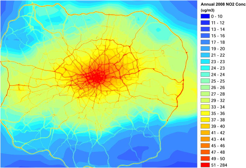
The predicted 2008 annual mean NO2 concentrations in London are shown in Fig. 1. These results show the heterogeneity of air pollution, with areas close to major roads visible as NO2 concentrations of greater than ∼40 μg m−3. NO2 (and NOX) concentrations also decrease according to distance from central London, where the highest concentrations occur and at suburban background locations concentrations of NO2 are ∼15 μg m−3. As expected, the spatial distribution of O3 concentrations (not shown) show the opposite of the NO2 concentration pattern, with the minimum concentration being in the central urban area and close to road sources.
Fig. 1.
Annual 2008 mean NO2 concentrations for London (μg m−3).
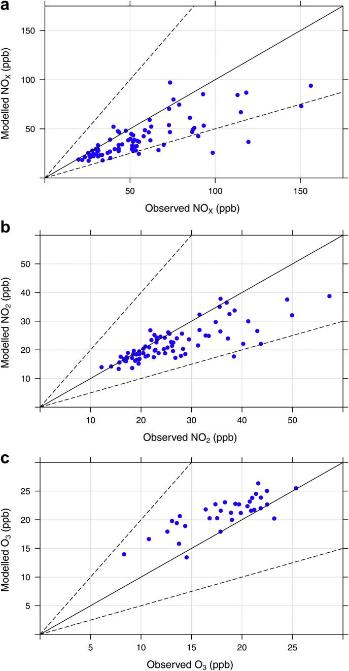
The annual mean scatter plots of NOX, NO2 and O3 are given in Fig. 2 and include a 1:1 solid black line and 1:0.5 and 1:2 dashed lines. The scatter plots in Fig. 2 show that whilst at background locations the model performs reasonably well, under predicting NOX and NO2 by ∼22% and 9%, respectively, the roadside and kerbside sites under predict observations by a larger margin of ∼32% and 22%, respectively. As expected, the opposite is true for O3 where there is an over prediction by the model, especially close to roads of ∼18%.
Fig. 2.
Scatter plots of annual mean NOX (a), NO2 (b) and O3 (c) concentrations (ppb) in London in 2006. The black line represents the 1:1 relationship and the dashed lines the 1:2 and 1:0.5 relationships.
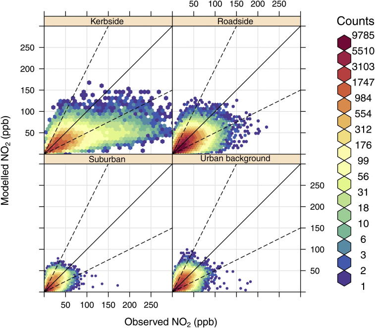
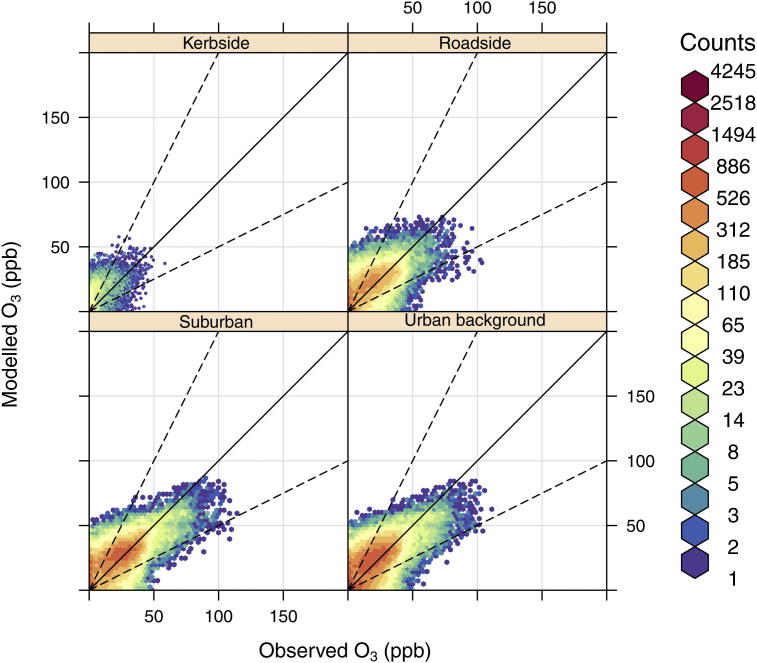
Scatter plots of the model vs. observed hourly NO2 and O3 concentrations, split into kerbside, roadside, suburban and urban background measurement site locations are shown in Figs. 3 and 4. Because it is difficult to distinguish the relationship in a scatter plot that includes thousands of points and uses only one colour, we have included a red to blue scale which reflects the number of hourly model–measurement pairs. The Figs. 3 and 4 show that the highest density of data (coloured red) is within ±FAC2 (dashed lines) for both NO2 and O3 and the results appear to show that the model predicts NO2 and O3 reasonably well at most site locations. However, a large negative bias in NO2 concentrations is observed at kerbside sites, especially at high concentrations, and a positive bias of O3 concentrations exists across all site types.
Fig. 3.
Scatter plots of hourly observed and modelled NO2 concentrations (ppb), at kerbside, roadside, urban background and suburban sites in 2006. The colour scale gives the hourly frequency within each scatter plot to allow clearer interpretation of the results. The black line represents the 1:1 relationship and the dashed lines the 1:2 and 1:0.5 relationships. (For interpretation of the references to colour in this figure legend, the reader is referred to the web version of this article.)
Fig. 4.
Scatter plots of observed and modelled O3 concentrations (ppb), at kerbside, roadside, urban background and suburban sites in 2006. The colour scale gives the hourly frequency within each scatter plot to allow clearer interpretation of the results. The black line represents the 1:1 relationship and the dashed lines the 1:2 and 1:0.5 relationships. (For interpretation of the references to colour in this figure legend, the reader is referred to the web version of this article.)
A summary of statistical measures of model performance, associated with Figs. 3 and 4, are shown in Table 1. FAC2 values indicate that for the ‘All sites’ category, more than 70% of modelled NO2 concentrations and 60% of modelled O3 concentrations are within factor of two of the observations. On average the model under predicts NO2 with a mean bias (MB) of approximately 5 ppb and a normalised mean bias (NMB) of −17%. The root mean squared error (RSME) and R value for NO2 are ∼18% and 0.6, respectively. In contrast, O3 is over predicted by approximately 3ppb giving a NMB of 15%, a RMSE of 12% and an r value of 0.64.
Table 1.
Statistical measures of model performance in 2006 at KS-kerbside sites, RS-roadside sites, SU-suburban sites and UB-urban background sites.
| Pollutant | Site | n | FAC2 | MB (ppb) | NMB | RMSE (%) | r |
|---|---|---|---|---|---|---|---|
| NO2 | All | 80 | 0.73 | −4.7 | −0.17 | 17.7 | 0.58 |
| O3 | All | 34 | 0.61 | 2.8 | 0.15 | 12.1 | 0.64 |
| NO2 | KS | 7 | 0.64 | −19.0 | −0.39 | 38.1 | 0.58 |
| NO2 | RS | 38 | 0.75 | −5.0 | −0.17 | 16.3 | 0.56 |
| NO2 | SU | 13 | 0.71 | −0.8 | −0.05 | 10.8 | 0.58 |
| NO2 | UB | 22 | 0.74 | −2.1 | −0.10 | 12.3 | 0.55 |
| O3 | KS | 1 | 0.37 | 5.6 | 0.68 | 11.1 | 0.50 |
| O3 | RS | 9 | 0.60 | 3.0 | 0.17 | 11.9 | 0.59 |
| O3 | SU | 10 | 0.66 | 2.7 | 0.13 | 12.4 | 0.65 |
| O3 | UB | 14 | 0.61 | 2.6 | 0.14 | 12.1 | 0.64 |
Overall the model vs. measured results, across the range of site categories, show that the model performance deteriorates as you move from background to roadside locations, with the kerbside sites showing the poorest performance of any site type. The evaluation of NO2 predictions at kerbside sites give the FAC2, MB, NMB, RMSE and r results of 0.64, −19 ppb, 0.39, 38% and 0.58, respectively, and represents an important reduction in performance, even when compared to roadside sites. Likewise the O3 results at kerbside locations are in poor agreement with observations.
4. Diagnostic evaluation of the CMAQ-urban model
Further diagnostic evaluation of the model has been used to establish the reasons for the model's performance in London. The diagnostic evaluation has focused on four areas: Hour of the week and month of the year temporal variations of NOX, NO2 and O3; comparison of the predicted and observed NOX, NO2 and O3 relationship at the Marylebone Road kerbside site; the impact of WRF wind speed predictions on modelled NOX, NO2 and O3 concentrations and the likely influence of the road traffic emissions used in the model.
4.1. Comparison of modelled and observed hourly NOX at Marylebone road
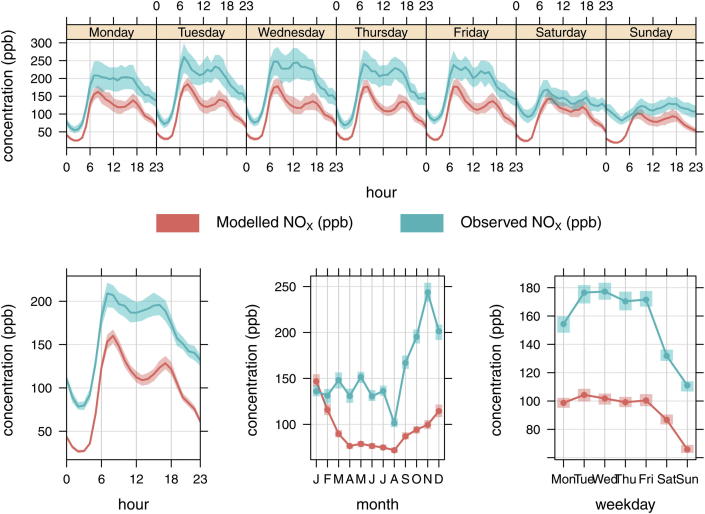
Hour of the week and month of the year modelled and observed NOX concentrations are plotted in Fig. 5 and show a negative bias across all periods of the week (top row plot) and a reasonable hourly emissions profile (bottom left plot). The consistent under prediction of NOX suggests that it is at least partly associated with an under prediction of road traffic NOX emissions. There is also evidence that the assumed reduction in emissions at weekends, compared with weekdays, is underestimated and does not compare well with measurements (bottom row right hand plot). Finally, the monthly bias increases during the period between September and December (bottom row middle plot) and this requires further investigation.
Fig. 5.
Observed and modelled NOX (ppb) at the Marylebone road kerbside site, for hour of the day, day of the week and month of the year. The shaded area represents the 95% confidence interval in the mean.
Evidence from the model results at Marylebone Road which suggest that road traffic NOX emissions are underestimated is supported by work undertaken by Carslaw et al. (2011a, 2011b) who showed that for 10 long running roadside NOX measurement sites in London, the period after 2004 had a median downward trend of between 0.6 and 1.7%/year and was associated with little or no improvement in the NOX emissions performance of light duty diesel vehicles. By comparing the emissions in London over the same period, Beevers et al. (2012) has shown the downward trend in NOX emissions for road traffic to be too large resulting in the under prediction of NOX emissions of ∼31% by 2008. This would suggest that NOX emissions in London (and the UK) are under predicted in 2006 by a large margin.
4.2. The effect of predictions of WRF wind speed on CMAQ-urban concentrations
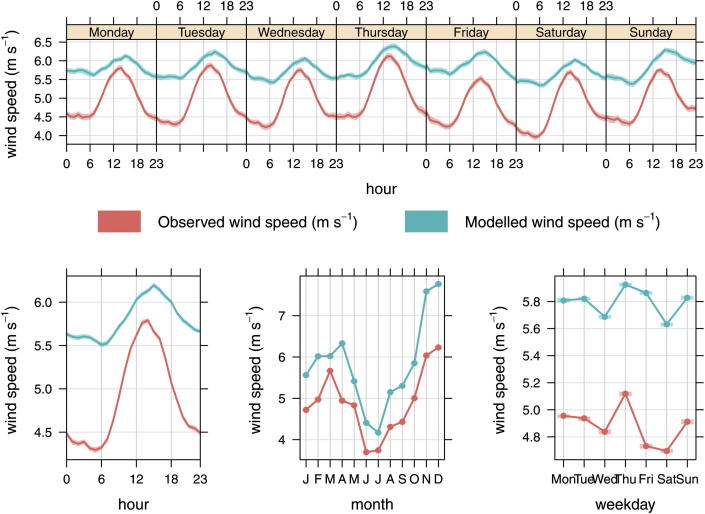
Modelled and observed wind speeds at 10 m height were compared at 147 ground based UK meteorological office stations (http://badc.nerc.ac.uk) summarised in Fig. 6. The sites are predominantly in rural locations, 103 of the 147, with 14 in urban locations and the rest coastal sites. The trend plots by hour of the week show that despite the use of observational nudging, there remains a positive bias in WRF predictions of wind speed compared with observations (top row plot). This is consistent with WRF predictions without nudging, which are not shown. The positive wind speed bias is small (∼9%) during the day, but during the overnight and morning periods the positive wind speed bias increases. Monthly comparisons also show that the bias increases slightly during winter months compared with the summer period (bottom row middle plot). Whilst, the results suggest that the model does not reflect the wind speed during overnight periods well, the nudging of temperature results in good agreement across all hours of week and months of the year.
Fig. 6.
Average WRF modelled (with observational nudging) and measured wind speeds (m s−1) for 147 ground based meteorological stations across the UK. The shaded area represents the 95% confidence interval in the mean.
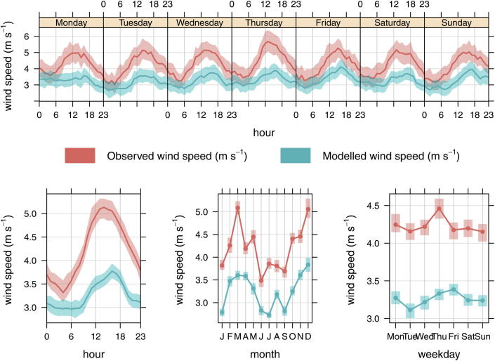
However, the performance of WRF at the London Heathrow site is different, and given that results at this site are likely to be more useful in interpreting the performance of CMAQ-urban we have separated out the WRF wind speed predictions at Heathrow and summarised them in Fig. 7. At Heathrow, using a combination of WRF and observational nudging has the effect of reducing the positive bias during the overnight period seen in Fig. 6, but causes the model to under predict the daytime wind speed by approximately 1.5 m s−1 (Fig. 7 – bottom row left plot). This is repeated at other UK urban sites. A reasonably consistent negative bias appears to exist by month of the year (bottom row middle plot) and by day of the week (bottom row right plot). The prediction of temperature at 2 m agrees with measurements at Heathrow for all hours of the week, with residuals (modelled–observed) being <0.5 °C, and reaching ∼1 °C during summer months.
Fig. 7.
Average WRF modelled and measured wind speeds at the Heathrow Airport ground based meteorological station close to London. The model includes observational nudging. The shaded area represents the 95% confidence interval in the mean.
The improvements in temperature predictions using observational nudging is reflected in increases in boundary layer heights compared with the without nudging case. However, a lack of observations of boundary layer height limits any conclusions that can be drawn about WRF's performance.
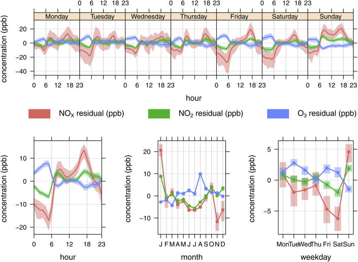
Assuming that the performance of WRF at Heathrow is reflected widely in London, we have sought to demonstrate the influence of WRF wind speed predictions on NOX, NO2 and O3 concentrations at the central London background monitoring site at Kensington and Chelsea. The reason for choosing a background site is that these data are less affected by any bias that local traffic emissions may have. The residual (modelled–observed) concentrations at Kensington and Chelsea are summarised in Fig. 8.
Fig. 8.
NOX, NO2 and O3 residuals (ppb) (modelled–observed) at the Kensington and Chelsea urban background monitoring site. The shaded area represents the 95% confidence interval in the mean.
The average hour of daytime series in the bottom left hand corner of Fig. 8 shows that during the morning period in particular there is a negative bias in NOX (and NO2) concentrations and this has lead to an over prediction of O3. The bias in NOX, NO2 and O3 are not likely to be linked with the WRF wind speed forecasts, which are well predicted during this period, and these results would suggest that the under prediction of road transport emissions of NOX are important at the Kensington monitoring site. The assumption that the CMAQ model bias during the early morning is driven by an under estimate in the NOX emissions inventory is further supported by the hour of week plot at the top of Fig. 8, which shows that Friday and Saturday morning in particular, are poorly predicted. Given that WRF wind speed predictions during all morning hours have a similarly small bias (Fig. 7) points to the NOX and NO2 emissions being the most likely cause. There is a positive bias in the model results during Sundays as well as a tendency to over predict during daytime periods in the remainder of the week (Fig. 8 – top row plot). During the daytime periods a negative bias in WRF predicted wind speed (Fig. 7) is one likely source of the error, and would counteract the effect of under predicting NOX emissions. The negative bias in wind speed during the day would also counteract the low emissions of NOX at Marylebone Road, discussed in Section 4.1. Finally, the monthly average residuals (bottom row middle plot) suggest that the model under predicts in November and December and over predicts during January for which further investigation is required.
4.3. The evaluation of a simple chemical scheme for predicting NO2 and O3 close to roads in London
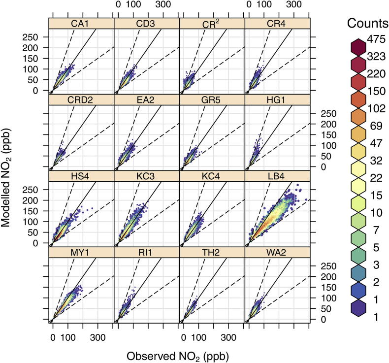
At roadside locations in London a simple NOX–NO2–O3 chemistry scheme has been used. Despite having been evaluated elsewhere, see Carslaw (2005) and Carslaw and Beevers (2005), we have evaluated the model in 2006 and 2008 using two approaches. First, we have compared the relationship between modelled and measured 2006 NO2 and O3 concentrations as a function of NOX at the Marylebone Road kerbside site and second, we have produced regression plots of the hourly NO2 predictions at 16 roadside sites in London, having constrained the model to the hourly NOX measurements.
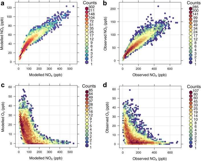
In the first analysis the hourly modelled and observed NO2 and O3 concentrations have been plotted against NOX concentrations and the results summarised in Fig. 9. The comparison between modelled (Fig. 9 (a)) and observed (Fig. 9 (b)) hourly NOX and NO2 concentrations show that the model tends to under predict both NOX and NO2 concentrations resulting in smaller concentration ranges. The maximum concentration of NOX is ∼500 ppb (model) and 600 ppb (observed) and for NO2 is ∼110 ppb (model) and 150 ppb (observed). The model also misses a large group of the highest NO2 concentrations (>80 ppb). The under prediction of NO2 at Marylebone Road is consistent with the results at other kerbside and roadside sites and with the under prediction of NOX and NO2 emissions discussed in Section 4.1.
Fig. 9.
Scatter plots of hourly observed and modelled NOX vs. NO2 and NOX vs. O3 (ppb) at the Marylebone Road kerbside site in 2006. The colour scale gives the hourly frequency within each scatter plot to allow clearer interpretation of the results. (For interpretation of the references to colour in this figure legend, the reader is referred to the web version of this article.)
The comparison between modelled (Fig. 9 (c)) and observed (Fig. 9 (d)) hourly NOX and O3 concentrations shows the model predicts a large number of O3 concentrations in the 0–150 ppb NOX range and 10–30 ppb O3 range, with the equivalent zone of observed concentrations having smaller numbers of hourly values. Furthermore, the zone with the highest number of observed O3 concentrations is in the ∼100–400 ppb NOX range and within the 0–5 ppb O3 range. This high number of low O3 concentrations is typical of kerbside locations, but is not replicated by the model which has a smaller number of the lowest O3 concentrations.
Whilst the comparison between NOX, NO2 and O3 for both modelled and observed concentrations is informative it is less helpful in identifying weaknesses in the chemistry model itself. Hence, for the second part of the chemistry scheme evaluation a regression analysis has been undertaken for each hour of 2008 at a subset of 16 London monitoring sites (Table 2), chosen to represent a complete range of roadside concentrations in London. In this case the model was constrained by using the measured hourly NOX concentrations at each site and the proportion of directly emitted NO2 from the LAEI, removing the uncertainty in predicting NOX and further isolating the chemical mechanism. The model vs. observed hourly NO2 concentrations are given as scatter plots in Fig. 10 and show good agreement, with the colour scale confirming that whilst scatter exists, the majority of points lie close to the 1:1 line. Regression statistics for the hourly NO2 concentrations give R2 values in the range of 0.81 (Camden 3) to 0.96 (Marylebone Road) and this confirms the good performance of the constrained model across virtually all sites. However, at the Croydon 2 site where the R2 value is 0.66, the model performs less well although the average NO2 concentrations are in close agreement. In contrast, at the Lambeth 4 site the model under predicts observations by 20%. However, Lambeth 4 sits 1–2 m from the kerb on a road with a frequent bus service, all of which have been fitted with regenerating particle traps and emit a large proportion of NOX as NO2 (Carslaw and Beevers, 2005), making this a difficult location to predict NO2. In conclusion, by isolating the NOX–NO2–O3 chemical scheme, we have demonstrated that the model compares well with roadside observations in London, despite its simplicity.
Table 2.
List of 16 roadside and kerbside sites used in the evaluation of the street scale NO–NO2–O3 chemistry model, including the R2 estimate between modelled and observed NO2 in 2008, the average modelled and observed NO2 in 2008 and the emissions based estimate of the exhaust NO2–NOX ratio.
| Site code | Site name | Site type | R2 | Observed NO2 (ppb) | Modelled NO2 (ppb) | Exhaust NO2:NOX |
|---|---|---|---|---|---|---|
| CA1 | Camden 1 – Swiss Cottage | Kerbside | 0.93 | 40 | 39 | 0.21 |
| CD3 | Camden 3 – Shaftesbury Avenue | Roadside | 0.81 | 41 | 38 | 0.19 |
| CR2 | Croydon 2 – Purley Way | Roadside | 0.66 | 24 | 24 | 0.16 |
| CR4 | Croydon 4 – George Street | Roadside | 0.84 | 26 | 26 | 0.26 |
| CRD2 | Kens and Chelsea 2 – Cromwell Rd | Roadside | 0.85 | 35 | 35 | 0.19 |
| EA2 | Ealing 2 – Acton Town Hall | Roadside | 0.85 | 29 | 31 | 0.24 |
| GR5 | Greenwich 5 – Trafalgar Road | Roadside | 0.83 | 27 | 26 | 0.22 |
| HG1 | Haringey 1 – Town Hall | Roadside | 0.87 | 19 | 21 | 0.23 |
| HS4 | Hounslow 4 – Chiswick High Rd | Roadside | 0.89 | 38 | 35 | 0.23 |
| KC3 | Kens and Chelsea 3 – Knightsbridge | Roadside | 0.92 | 48 | 49 | 0.24 |
| KC4 | Kens and Chelsea 4 – Kings Rd | Roadside | 0.86 | 48 | 50 | 0.26 |
| LB4 | Lambeth 4 – Brixton Road | Kerbside | 0.93 | 113 | 90 | 0.25 |
| MY1 | Marylebone Rd – Baker St | Kerbside | 0.96 | 61 | 55 | 0.20 |
| RI1 | Richmond 1 – Castlenau | Roadside | 0.89 | 23 | 23 | 0.24 |
| TH2 | Tower Hamlets 2 – Mile End Rd | Roadside | 0.90 | 32 | 29 | 0.20 |
| WA2 | Wandsworth Town hall | Roadside | 0.85 | 25 | 26 | 0.21 |
Fig. 10.
Scatter plots of hourly model vs. measured NO2 (ppb) at 16 roadside and kerbside sites in London. The colour scale gives the hourly frequency within each scatter plot to allow clearer interpretation of the results. The black line represents the 1:1 relationship and the dashed lines the 1:2 and 1:0.5 relationships. (For interpretation of the references to colour in this figure legend, the reader is referred to the web version of this article.)
5. Double counting
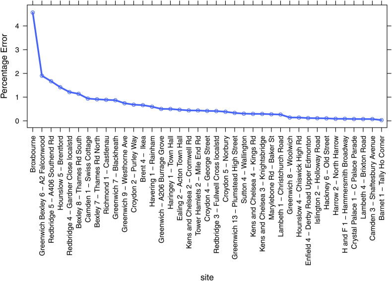
As a consequence of coupling the CMAQ and ADMS models a degree of double counting exists. The reason for this is that the CMAQ model, used for the background concentration estimates, includes all of the emissions sources in London and superimposed upon this background is the ADMS predicted concentrations, which use emissions from the major roads in London. Hence we are effectively counting the major road emissions twice. However, we have demonstrated that this has limited influence on the model predictions, by first, limiting the spatial domain of the roadside model to 225 m from each road source. The 225 m limit in this case is taken to be the limit at which one can measure the annual average influence of a single road above background concentrations and beyond 225 m of a road, the CMAQ concentrations remain unchanged. However, it is accepted that the applicability of the 225 m limit will depend on atmospheric stability and for some hours of the year the local influence of major roads will extend well beyond this limit. Second, whist we accept that some double counting still exists close to roads, it can be tested in a straight forward way. To do this we have used the NOX emissions and observations at 39 roadside and kerbside sites closest to the largest roads in London. For each measurement site the 2006 NOX emissions and length of road was taken from the LAEI. Where a single road was >3 km long in the LAEI the length was limited to 3 km to be consistent with the size of the CMAQ grids. Using the LAEI estimate, an equal mass of NOX emissions was released into a volume source of dimensions 3 km × 3 km × 14 m, equivalent to the lowest layer in the CMAQ model, and the volume source average concentration predicted using the ADMS volume source model (v4.1). The volume average concentration, which represents the magnitude of the double counting effect, was then expressed as a percentage of the roadside NOX measurements and the results summarised in Fig. 11.
Fig. 11.
The percentage error in the CMAQ-urban model associated with double counting NOX emissions at 39 London roadside sites.
The results of double counting show a small range at most of the roadside locations with the median percentage error of 0.42% across all sites. This represents a very small error and of little importance in predicting roadside concentrations. One site (Broxbourne) has a larger percentage error of 4.5%, and this is a site outside of the M25 motorway, one of the largest traffic sources in the UK. The site is also at ∼60 m from the centre of the motorway and so sits between a roadside and background site location. At this location the M25 motorway passes through an area of relatively low NOX emissions, from other sources, and as such the site represents a worst case location for double counting. Despite the worst case location the error of 4.5% is approximately half the magnitude of the measurement error for NOX.
6. Conclusions
A coupled CMAQ and ADMS modelling system, CMAQ-urban, has been developed for London to give fine temporal and spatial scale (hourly and 20 m × 20 m) NOX, NO2 and O3 concentrations. The model used a combination CMAQ v4.6 to predict background concentrations and the ADMS roads model (v2.3) to represent the dispersion from road traffic. Highly detailed road traffic emissions were taken from the LAEI 2006 and 2008 and the model evaluated against 80 measurement sites in London. The majority of tests were undertaken for 2006, although some results for 2008 are presented to support the model evaluation.
The model was able to capture the spatial heterogeneity of NO2 and O3 concentrations across London. Using observations from 80 monitoring sites at locations which included urban background, suburban, roadside and kerbside sites, the model predicted NO2 and O3 concentrations reasonably well, although at kerbside sites the model under predicted NO2 by a large margin and especially at high hourly concentrations.
By using diagnostic tests such as average modelled and measured concentrations by month of the year and hour of the week, for WRF and CMAQ, we have been better able to differentiate the likely source of model error. For example, the under prediction of NOX and NO2 concentrations at the Kensington and Chelsea urban background sites during the overnight period is likely to be a result of underestimated road traffic NOX emissions, which is also reported elsewhere (Carslaw et al., 2011a), whilst the over prediction of NOX concentrations during the day at Kensington is a combination of under prediction of wind speed and underestimated road traffic NOX emissions.
The contrast in WRF performance across the UK, which are dominated by rural locations, and those in more urban settings such as Heathrow is confusing and is likely to be as a consequence of the effectiveness of the observational nudging approach adopted within the model. The initial aim of nudging was to resolve the (un-nudged) WRF positive bias in overnight wind speed. However, observational nudging proved to be ineffective at the majority of rural sites, where the over prediction of wind speed remained, but was influential at urban sites such as Heathrow. The unintended consequence of using nudging was to artificially create one negative bias (daytime at Heathrow), whilst attempting to solve the overnight positive bias. The performance of WRF is very important if good CMAQ model performance is to be achieved and care should be taken when using nudging techniques with the WRF model.
A comprehensive evaluation of the simple chemistry model used to predict roadside NO2 and O3 has been reported elsewhere (Carslaw and Beevers, 2005). However, by constraining the model using measured NOX concentrations, and effectively isolating the chemical scheme we have shown the model to be able to predict the hourly NO2 very well close to roads, despite its simplicity. This is a reflection of the limited time available for other atmospheric components, such as VOC's, to significantly influence concentrations such as O3 and also reflects the modest level of photochemistry experienced in the UK. Hence care should be taken when applying the model to a range of climates.
The influence of double counting was also tested comprehensively across 39 roadside and kerbside sites and for the vast majority of sites this effect is very small. The median double counting error represents 0.42% of the roadside concentration of NOX. At a ‘worst case’ location close to one of the UK's largest motorways the error of 4.5% of roadside concentrations is still half of the measurement error of NOX. This is an important finding as it confirms that the one way coupling method described is reasonable, simplifies the combination of the local scale and regional scale models and does not influence the workings of the CMAQ model itself.
The double counting error incurred by coupling the two models is also likely to be smaller for other pollutants such as PM, given that the addition of PM10 exhaust and PM10 non-exhaust emissions are approximately 5–10% of NOX. In addition, by coupling the models, use can be made of larger grid sizes without loss of predictive capability. For example, approximately the same results of NOX, NO2 and O3 concentrations in London can be obtained using a CMAQ grid of 9 × 9 km, instead of 3 × 3 km, which has the potential to reduce the double counting error by up to a factor of 9 as well as reducing the CMAQ run times.
Any number of additional reasons could be made for the errors occurring at locations close to road traffic, such as the effect of multi-lane roads and the existence of tidal traffic flows, the simplicity of ADMS roads model and the street canyon model within it, as well as defining street canyon characteristics, all of which are potential sources of error. These have not been investigated in this paper and will be the subject of future analysis.
Despite the model errors discussed, we have demonstrated that the use of CMAQ-urban for the prediction of O3 and NOX/NO2 concentrations in London is promising. And that at the spatial and temporal scale described this model can be used for health impact assessments, epidemiological study, detailed human exposure assessments and to assess compliance with air quality legislation. Finally, forecasts of PM concentrations, using similar methods and version 5 of CMAQ, will be the subject of future work.
Acknowledgements
The authors would like to acknowledge USEPA and NCEP/NCAP for CMAQ/WRF models, Department of Environment, Food and Rural Affairs (DEFRA) for the UK emissions and monitoring data and King's College for road traffic emissions and monitoring data in London. Also thanks go to the AQMEII project for use of their hourly emissions profiles. We also acknowledge the Natural Environment Research Council, Medical Research Council, Economic and Social Research Council, Department of Environment, Food and Rural Affairs and Department of Health for the funding received for the Traffic Pollution and Health in London project (NE/I008039/1), funded through the Environmental Exposures & Health Initiative (EEHI).
References
- AEA . DEFRA; 2009. Evaluating the Performance of Air Quality Models. AEAT/ENV/R/2793. [Google Scholar]
- Ashmore M. 2005. Quantification of Population Exposure Benefits of Reducing Roadside and Urban Background Pollution Concentrations Final Report March 2005 (Reports of the UK Department of Health Policy Research Programme)http://collections.europarchive.org/tna/20100509080731http://www.dh.gov.uk/prod_consum_dh/groups/dh_digitalassets/@dh/@en/documents/digitalasset/dh_092835.pdf Available at: (accessed 19.07.11.) [Google Scholar]
- Beevers S.D., Westmoreland E., de Jong M.C., Williams M.L., Carslaw D.C. Trends in NOX and NO2 emissions from road traffic in Great Britain. Atmospheric Environment. 2012;54:107–116. [Google Scholar]
- Builtjes P. 2005. Review of Methods for Assessing Air Quality at Regional/Continental Scale. 6th Framework Programme: Air4EU, Deliverable D5.1. [Google Scholar]
- Byun D.W., Ching J.K.S. U.S. Environmental Protection Agency, Office of Research and Development; 1999. Science Algorithms of the EPA Models-3 Community Multiscale Air Quality (CMAQ) Modeling System. EPA/600/R-99/030. [Google Scholar]
- Carslaw D.C., Beevers S.D. Estimations of road vehicle primary NO2 exhaust emission fractions using monitoring data in London. Atmospheric Environment. 2005;39:167–177. [Google Scholar]
- Carslaw D.C., Ropkins K. Openair – an R package for air quality data analysis. Environmental Modelling & Software. 2012;27–28:52–61. [Google Scholar]
- Carslaw D.C., Beevers S.D., Tate J.E., Westmoreland E., Williams M.L. Recent evidence concerning higher NOx emissions from passenger cars and light duty vehicles. Atmospheric Environment. 2011;45:7053–7063. [Google Scholar]
- Carslaw D.C., Beevers S.D., Westmoreland E., Williams M.L., Tate J.E., Murrells T., Stedman J., Li Y., Grice S., Kent A., Tsagatakis I. 2011. Trends in NOX and NO2 Emissions and Ambient Measurements in the UK.http://uk-air.defra.gov.uk/library/reports?report_id=673 Version: July 2011. (accessed 31.05.11.) [Google Scholar]
- Carslaw D.C. Evidence of an increasing NO2/NOX emissions ratio from road traffic emissions. Atmospheric Environment. 2005;39(26):4793–4802. (accessed 03.11.11.) [Google Scholar]
- Carslaw D.C. 2011. DEFRA Urban Model Evaluation Analysis – Phase 1.http://uk-air.defra.gov.uk/library/reports?report_id=654 (accessed 13.12.11.) [Google Scholar]
- CERC . Cambridge Environmental Research Consultants Ltd; Cambridge: 2006. AMDS-Roads an Air Quality Management System User Guide.http://www.cerc.co.uk/environmental-software/assets/data/doc_userguides/CERC_ADMS-Roads%20Extra3.1_User_Guide.pdf (accessed 03.01.12.) [Google Scholar]
- Chang J.C., Hanna S.R. Air quality model performance evaluation. Meteorology and Atmospheric Physics. 2004;87:167–196. [Google Scholar]
- Chen F., Dudhia J. Coupling an advanced land-surface/hydrology model with the Penn State/NCAR MM5 modeling system. Part I: model description and implementation. Monthly Weather Review. 2001;129:569–585. [Google Scholar]
- EC Directive 2008/50/EC, ambient air quality and cleaner air for Europe. Official Journal of the European Communities. 2008 L 152/1, 11 June 2008. [Google Scholar]
- Georgopoulos A source-to-dose assessment of population exposure to fine PM and ozone in Philadelphia, PA, during a summer 1999 episode. Journal of Exposure Analysis and Environmental Epidemiology. 2005;15:439–457. doi: 10.1038/sj.jea.7500422. [DOI] [PubMed] [Google Scholar]
- Greater London Authority (GLA) 2010. The London Atmospheric Emissions Inventory 2008.http://data.london.gov.uk/laei-2008 (accessed 31.05.11.) [Google Scholar]
- Greater London Authority (GLA) 2010. Cleaning the Air.http://www.london.gov.uk/sites/default/files/Air%20Quality%20Strategy%20v3.pdf (The Mayors Air Quality Strategy). (accessed 31.05.11.) [Google Scholar]
- Grice S., Stedman J., Kent A., Hobson M., Norris J., Abbott J., Cooke S. Recent trends and projections of primary NO2 emissions in Europe. Atmospheric Environment. 2009;43(13):2154–2167. http://www.sciencedirect.com/science/article/B6VH3-4VDS8MT-3/2/4a692307ac35ebf6ba37560cf32b4cf9 [Google Scholar]
- Guenther A., Hewitt C.N., Erickson D., Fall R., Geron C., Graedel T., Harley P., Klinger L., Lerdau M., McKay W.A., Pierce T., Scholes B., Steinbrecher R., Tallamraju R., Taylor J., Zimmerman P. A global model of natural volatile organic compound emissions. Journal of Geophysical Research. 1995;100:8873–8892. [Google Scholar]
- Hong S.-Y., Noh Y., Dudhia J. A new vertical diffusion package with an explicit treatment of entrainment processes. Monthly Weather Review. 2006;134:2318–2341. [Google Scholar]
- Isakov V., Touma J.S., Burke J., Lobdell D., Palma T., Rosenbaum A., Özkaynak H. Combining regional- and local-scale air quality models with exposure models for use in environmental health studies. Journal of the Air & Waste Management Association. 2009;59:461–472. doi: 10.3155/1047-3289.59.4.461. [DOI] [PubMed] [Google Scholar]
- Kain J.S. The Kain–Fritsch convective parameterization: an update. Journal of Applied Meteorology. 2004;43:170–181. [Google Scholar]
- Kelly F.J., Anderson H.R., Armstrong B., Atkinson R.W., Barratt B., Beevers S.D., Mudway I.S., Green D., Derwent R.G., Tonne C., Wilkinson P. Health Effects Institute; 2011. The Impact of the Congestion Charging Scheme on Air Quality in London.http://pubs.healtheffects.org/view.php?id=358 [PubMed] [Google Scholar]
- Maheswaran R., Pearson T., Smeeton N.C., Beevers S.D., Campbell M.J., Wolfe C.D. Impact of outdoor air pollution on survival after stroke population-based cohort study. Stroke. 2010 doi: 10.1161/STROKEAHA.109.567743. [DOI] [PubMed] [Google Scholar]
- Mlawer E.J., Taubman S.J., Brown P.D., Iacono M.J., Clough S.A. Radiative transfer for inhomogeneous atmosphere: RRTM, a validated correlated-k model for the longwave. Journal of Geophysical Research. 1997;102(D14):16663–16682. [Google Scholar]
- Molitor J., Su J.G., Molitor N.T., Rubio V.G., Richardson S., Hastie D., Morello-Frosch R., Jerrett M. Identifying vulnerable populations through an examination of the association between multipollutant profiles and poverty. Environmental Science and Technology. 15 Sep 2011;45:7754–7760. doi: 10.1021/es104017x. http://dx.doi.org/10.1021/es104017x [DOI] [PubMed] [Google Scholar]
- Murrells T.P., Passant N.R., Thistlethwaite G., Wagner A., Li Y., Bush T., Norris J., Walker C., Stewart R.A., Tsagatakis I., Whiting R., Conolly C., Okamura S., Peirce M., Sneddon S., Webb J., Thomas J., MacCarthy J., Choudrie S., Brophy N. Report Produced for Department for Environment, Food and Rural Affairs (DEFRA); 2010. UK Emissions of Air Pollutants 1970 to 2008.http://uk-air.defra.gov.uk/reports/cat07/1009030925_2008_Report_final270805.pdf (accessed 31.05.11.) [Google Scholar]
- NEDC . 2001. Directive 2001/81/EC of the European Parliament and of the Council, on National Emissions Ceilings for Certain Atmospheric Pollutants.http://ec.europa.eu/environment/air/pollutants/ceilings.htm (accessed 03.11.11.) [Google Scholar]
- Roselle, S.J., Schere, K.L., Pleim, J.E., 1999. Chapter 14: photolysis rates for CMAQ. In: Science Algorithms of the EPA Models-3 Community Multiscale Air Quality (CMAQ) Modeling System. EPA/600/R-99/030.
- Sanderson M.G. UK Meteorological Office; 2002. Emission of Isoprene, Monoterpenes, Ethene and Propene by Vegetation. Hadley Centre Technical Note 40. [Google Scholar]
- Shao X., Stein M., Ching J. Statistical comparisons of methods for interpolating the output of a numerical air quality model. Journal of Statistical Planning and Inference. 2007;137:2277–2293. [Google Scholar]
- Skamrock W.C., Klemp J.B., Dudhia J., Gill D.O., Barker D.M., Duda M.G., Huang X.-Y., Wang W., Powers J.G. 2008. A Description of the Advanced Research WRF Version 3. NCAR/TN–475+STR. [Google Scholar]
- Tonne C., Beevers S.D., Kelly F.J., Jarup L., Wilkinson P., Armstrong B. An approach for estimating the health effects of changes over time in air pollution: an illustration using cardio-respiratory hospital admissions in London. Occupational and Environmental Medicine. 2010;67:422–427. doi: 10.1136/oem.2009.048702. [DOI] [PMC free article] [PubMed] [Google Scholar]
- UNECE . 1999. United Nations Economic Commission for Europe, Convention on Long Range Transboundary Air Pollution.http://www.unece.org/env/lrtap/multi_h1.html Protocol to Combat Acidification, Eutrophication and Ground-level Ozone, United Nations, Geneva. (accessed 03.11.11.) [Google Scholar]
- Woodcock J., Roberts I., Edwards P., Armstrong B., Banister D., Beevers S.D., Chalabi Z., Cohen A., Franco O., Haines A., Hickman R., Lindsay G., Mittal I., Mohan D., Tiwari G., Tonne C., Woodward A. Impact on public health effects of strategies to reduce greenhouse gas emissions: urban land transport. Lancet. 2009;374:1930–1943. doi: 10.1016/S0140-6736(09)61714-1. [DOI] [PubMed] [Google Scholar]
- Yarwood G., Rao S.T., Yocke M., Whitten G. US EPA, Res. Tri. Park; 2005. Updates to the Carbon Bond Chemical 476 Mechanism: CB05, Report, Rpt. RT-0400675. [Google Scholar]


