Histology image analysis for carcinoma detection and grading

Abstract

This paper presents an overview of the image analysis techniques in the domain of histopathology, specifically, for the objective of automated carcinoma detection and classification. As in other biomedical imaging areas such as radiology, many computer assisted diagnosis (CAD) systems have been implemented to aid histopathologists and clinicians in cancer diagnosis and research, which have been attempted to significantly reduce the labor and subjectivity of traditional manual intervention with histology images. The task of automated histology image analysis is usually not simple due to the unique characteristics of histology imaging, including the variability in image preparation techniques, clinical interpretation protocols, and the complex structures and very large size of the images themselves. In this paper we discuss those characteristics, provide relevant background information about slide preparation and interpretation, and review the application of digital image processing techniques to the field of histology image analysis. In particular, emphasis is given to state-of-the-art image segmentation methods for feature extraction and disease classification. Four major carcinomas of cervix, prostate, breast, and lung are selected to illustrate the functions and capabilities of existing CAD systems.

1. Introduction

Histology is the study of the microscopic anatomy of cells and tissues of organisms. Histological analysis is performed by examining a thin slice (section) of tissue under a light (optical) or electron microscope [47,74,80,104,127]. In the present research, the study of histology images is regarded as the gold standard for the clinical diagnosis of cancers and identification of prognostic and therapeutic targets. Histopathology, the microscopic study of biopsies to locate and classify disease, has roots in both clinical medicine and in basic science [104]. In histology image analysis for cancer diagnosis, histopathologists visually examine the regularities of cell shapes and tissue distributions, decide whether tissue regions are cancerous, and determine the malignancy level. Such histopathological study has been extensively employed for cancer detection and grading applications, including prostate [41,42,105,106,108], breast [6,43,109], cervix [56,57,79,122], and lung [75,78,87,131] cancer grading, neuroblastoma categorization [61,81,83,84], and follicular lymphoma grading [34,82,134]. In this paper we use examples of one class of cancers that originates from epithelial cells, i.e., carcinoma, to illustrate common histopathology image analysis functions. For other cancers, for example, sarcoma from muscle cells [19,99], melanoma from melanocytes of the skin [14,32,46], or astrocytoma from brain cell [51,59], interested readers are referred to the references. These various applications share similar computer techniques to support clinicians by automatic histology image feature extraction and classification.

As for radiology and cytology image analysis, histopathology problems attract researchers from the disciplines of clinical medicine, biology, chemistry, and computing. Computer-based image analysis has become an increasingly important field because of the high rate of production and the increasing reliance on these images by the biomedical community. Medical image processing and analysis in radiology (e.g. X-ray, ultrasound, computed tomography (CT), and magnetic resonance image (MRI)) and cytology have been active research fields for several decades, and numerous systems [5,55,65,158] and products^1,2,3 [72,90] have been developed. However, the use of these systems in histology analysis is not straightforward due to the significantly different imaging techniques and image characteristics. Fig. 1 shows one example for CT, cytology, and histology images. Histology images differ from radiology images in having a large amount of objects of interest (cells and cell structures, such as nuclei) widely distributed and surrounded by various tissue types (for example, in the cervix, epithelium and stroma). In contrast, radiology image analysis usually focuses on a few organs in the image,⁴ which tend to be more predictably located. A histology image usually has a size (~10⁹ pixels) significantly larger than that of a radiology image (~10⁵ pixels). In addition, histology tissues are generally stained with different colors while radiology images usually contain only gray intensities. Cytology images have some similarities to histology images; both have multiple cells distributed in the images. However, histology images are usually taken at a much lower magnification level. This lower magnification allows analysis at the tissue level, such as classification of epithelium versus stroma, and identification of the boundary between tissue types; the histology magnification level is sufficient to allow some analysis at the cell level, such as nucleus counting and identification of gross deformities in the nucleus, but cannot provide the in-depth information of internal cell structure available to cytology. The complexity of histological images is driven by several factors, including overlapping tissue types and cell boundaries and nuclei corrupted by noise; some structures, such as cell boundaries, may appear connected or blurred. These factors make it rather difficult to extract cell regions (e.g. nuclei and cytoplasm) by traditional image segmentation approaches. On the other hand, cytology images are taken at a high magnification level which results in clearly identified cell “compartments”. Computer-based histology analysis systems generally exploit a much larger quantity of image features to derive clinically meaningful information than similar systems for radiology and cytology. Nevertheless, the image analysis systems for these three domains generally consist of a common sequence of steps of image restoration, segmentation, feature extraction, and pattern classification (see Section 3).

Fig. 1.

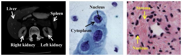
Image examples for radiology CT (left), cytology (middle), and histology (right) (Fig. 1 of [69]).

While histology image interpretation continues to be the standard for cancer diagnosis, current computer technology towards this task falls behind clinical need. Manual analysis of histology tissues is still the primary diagnosis method, and depends heavily on the expertise and experience of histopathologists. Such manual intervention has the disadvantages of (a) being very time consuming and (b) being difficult to grade in a reproducible manner; empirically, it is known that there are substantial intra- and inter-observation variations among experts. Factors which impede the development of effective computer-based histology analysis include: (a) the large diversity and high complexity of histology traits make it difficult to develop a universal computer system to analyze images of different cancers; (b) the fact that advanced image processing systems for radiology and cytology applications cannot be directly adopted for histology images due to the different imaging technologies and image characteristics; (c) the scarcity of “ground truth” for cancerous tissue identification and classification, which makes algorithm evaluation largely subjective or only dependable to minimal confidence testing. Nonetheless, the large and impractical demands on experts’ time to interpret the images are making computer assisted diagnosis (CAD) systems increasingly important. Compared to manual analysis, computer-based systems may provide rapid and consistent cancer detection and grading results. In this paper, we choose four major carcinomas, i.e., lung, prostate, breast, and cervix, as examples of histology image analysis for cancer detection and grading. Although a number of research papers on histology image interpretation and analysis have been published, few of these specifically survey image processing methods for histology analysis [2,60,95,110,115,155], and these usually focus on specific domain users such as computer scientists [2,115] or clinicians [95,110]. In addition, most works do not provide an up-to-date introduction to current advanced image analysis techniques. To meet the needs of a larger range of users, we aim to provide an overview of recent image analysis techniques in the domain of histopathology, in addition to the relevant background information about the technical procedures for tissue image production. For histology image analysis, besides a general description of current CAD functional modules as in the recent survey [60], we also provide a detailed, though introductory, example of the image segmentation module, by illustrating the performance of our methods and nine commonly used approaches. In particular, with a real histology image, we provide both qualitative and quantitative performance comparisons of the selected methods. Implicit in the comparative results that we provide is our effort in constructing a standard dataset to benchmark different algorithms. This addresses the issue of the scarcity of standard datasets and ground truth of histology applications for segmentation validation. Last but not least, we introduce practical histology cases (four carcinomas) and products to show real world CAD applications. We hope that our description of histology imaging technologies and major histopathology problems will provide important and challenging research topics for computer scientists.

This paper is organized as follows. Section 2 briefly introduces the technical procedures and several imaging technologies to prepare and produce digitized histology images. Section 3 presents the functional modules of commonly used CAD systems for histology image analysis, with a detailed introduction to current major image segmentation methods. Section 4 reviews the CAD systems for the four selected carcinomas detection and classification. We summarize this paper in Section 5.

2. Background

A histology image analysis system generally consists of a complex combination of hardware and software [155]. We roughly divide it into two sequential subsystems: (a) tissue preparation and image production; followed by (b) image processing and analysis. In this section we introduce the first subsystem, including several major histology imaging technologies. Fig. 2 shows the overall functions of the first subsystem. More details of the subsystem can be seen in our earlier work [69]. Current image processing and analysis techniques will be reviewed in Section 3.

Fig. 2.

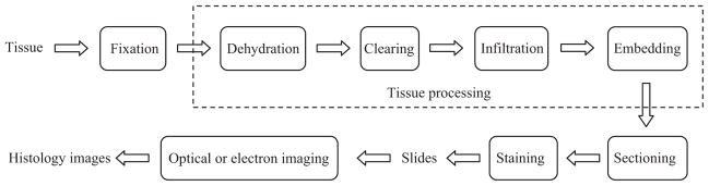
Histology tissue preparation and image production (Fig. 2 of [69]).

2.1. Histology tissue preparation procedures

After collecting tissue samples in vivo (e.g. for surgical pathology), fixation is the first stage of preparation for subsequent procedures, which should be conducted in real time to preserve the samples as well as possible. Depending on the imaging and analysis goals, different fixatives (e.g. precipitant and crosslinking) or methods (e.g. heat fixation and immersion) may be used. For example, the precipitant fixatives (e.g. methanol, ethanol, acetone, and chloroform) dehydrate the tissue samples, removing lipid and reducing the solubility of proteins. After fixation, the tissue must be adequately supported, e.g. frozen or embedded in a solid mold, to allow sufficiently thin sections to be cut for microscopic examination. Common treatments employ a series of reagents to process the fixed tissue and embed it in a stable medium such as paraffin wax, plastic or resin. Such treatments include the main steps of dehydration, clearing, infiltration, and embedding [28,111,155]. The embedded tissue sample is finally cut into thin sections (e.g. 5 μm for light microscopy and 80–100 nm for electron microscopy) to be placed on a slide. The transparent sections are usually produced with a microtome, an apparatus feeding the hardened blocks through a blade with high precision. After cutting, the sections are floated in warm water to smooth out any wrinkles. Then they are mounted (by heating or adhesives) on a glass slide ready for staining, which helps to enhance the contrast and highlight specific intra- or extra-cellular structures. A variety of dyes and associated staining protocols are used. The routine stain for light microscopy is hematoxylin and eosin (H&E); other stains are referred to as “special stains” for specific diagnostic needs. Each dye binds to particular cellular structures, and the color response to a given stain can vary across tissue structures. For example, hematoxylin stains the nuclear components of cells dark blue and eosin stains the cytoplasmic organelles varying shades of pink, red or orange. A detailed description of common laboratory stains can be seen in [80,127]. After staining, a coverslipping procedure is applied to cover the stained section on the slide with a thin piece of plastic or glass to protect the tissue and provide better visual quality for microscope examination.

2.2. Histology imaging technologies

After the tissue preparation process, light and electron microscopes, equipped with a variety of imaging technologies [107,144], are used to take digital histology images on the stained sections.

2.2.1. Light microscopy

The light microscope is the most commonly used instrument to magnify the tissue structures and produce high-resolution histology images. The essential components of a light microscope include an illumination system and an imaging system. The illumination system uses visible light to uniformly highlight the tissue slide; it either transmits light through the sample, or provides reflected light from the sample. This light then passes through one or multiple lenses of the imaging system. The resulting magnified view of the sample is either observed directly by the operator or captured digitally by a CCD camera.

Fluorescence microscopy

Fluorescence microscopy [52,71,94] is used to examine specimens using the absorption and subsequent re-radiation phenomena of fluorescence or phosphorescence. The emission of light through the fluorescence process is nearly simultaneous with the absorption of the excitation light due to a relatively short time delay (less than 1 μs) between photon absorption and emission. Since most tissue specimens do not fluoresce by themselves, a fluorescent molecule called a fluorophore (or fluorochrome) is needed to label the objects of interest such as molecules or subcellular components. A single fluorophore (color) is imaged at a time, and a multi-color image of several fluorophores is constructed by combining several single-color images. Variations and extensions of fluorescence microscopy include immunofluorescence microscopy [124], and two- or multi-photon microscopy [38,96,113].

Confocal microscopy

Confocal microscopy [107,118] restricts the final image to the same focus as the point of focus (i.e., focal plane) in the specimen, so that the objects of interest are “confocal”. Specifically, the out-of-focus light that originates in objects above or below the focal plane is filtered out with a spatial pinhole. Traditionally, the signal produced by normal fluorescence microscopy is from the full thickness of the specimen, which does not allow most of it to be in focus to the observer. In contrast, a confocal microscope uses point illumination and a pinhole situated in front of the image plane, which acts as a spatial filter and allows only the in-focus portion of the light to be imaged. As only light produced by fluorescence very close to the focal plane can be detected, the image resolution is much better than that of traditional fluorescence microscopes. However, since the amount of light from sample fluorescence is greatly blocked (up to 90–95%) at the pinhole, the intensity of the final image is significantly decreased. This can be compensated for with a stronger light source such as laser, a longer exposure, or a highly sensitive photosensor. Since only a single point of excitation light (or sometimes a group of points) is applied, 2D or 3D imaging requires scanning across the specimen, e.g. a rectangular raster.

Hyperspectral and multispectral microscopy

In recent years, biologists and pathologists have begun to exploit hyperspectral and multispectral imaging technologies [18,29,100,123] for microscopy image analysis. These technologies employ visible light, as well as ultraviolet and infrared, to acquire more comprehensive information from specimens. With this richer data, tissue constituents can be more easily identified by using their unique spectral signatures. Each hyperspectral or multispectral image is a 3D data cube with an extra spectral coordinate representing the wavelength of the excitation light. Hyperspectral data is usually a set of contiguous bands collected by one sensor, and multispectral is a set of discrete spectral bands that are optimally chosen and can be collected from multiple sensors. The primary disadvantages of these technologies are high cost and complexity for processing and storage.

2.2.2. Electron microscopy

Because of diffraction and aberrations of the optical system, a light microscopy image is usually not identical with the original sample. Moreover, the wavelength of the applied visible light limits the resolution of a light microscope (approximately 200 nm), which can differentiate cells but not the details of cell organelles. For higher resolution, more expensive electron microscopy [86,107] is needed; this technology employs electrons to “illuminate” specimens with a much smaller wavelength (less than 1 nm). The electrons can be generated by applying a high voltage to a hot wire; they are then accelerated by a high electric field and focused by electromagnets. After penetrating a sample, the electrons are diffracted to form a diffraction pattern, which is then transformed with a lens to obtain the sample image.

Transmission electron microscopy (TEM)

TEM transmits a beam of electrons through a specimen; the specimen-modulated beam is then detected by a fluorescent screen, and can be recorded on film. Since electrons interact strongly with matter, very thin sections (less than 100 nm) are needed to avoid large attenuation when the electrons pass through the slide. Based on TEM, high resolution electron microscopy (HREM) was invented; HREM uses “phase-contrast” techniques to achieve a resolution of approximately 0.2 nm, which is sufficient to provide atomic-scale resolution.

Scanning electron microscopy (SEM)

SEM transmits a fine beam of electrons onto a specimen and collects the secondary electrons that are reflected by the sample surface to produce a 3D image, i.e., an intensity map as a function of electron-beam position. Therefore, larger and thicker structures can be seen under the SEM as the electrons do not have to pass through the sample in order to form the image. This has poorer resolution than TEM, but is useful for studying surface morphology or measuring particle size. Nonconductive samples require an evaporated gold or graphite coating over the sample to prevent charging effects that would distort the electric fields in the electron microscope.

3. Histology image processing and analysis

After the tissue preparation and image production through different imaging technologies, the resulting digital histology images are ready for analysis by clinicians or CAD systems. As indicated in Section 1, manual analysis is generally very time consuming depending on the experience levels of the histopathologists. In addition, the inconsistent and variable responses from the observers, including both intra- and inter-observer variations, are not uncommon in practice. To ameliorate these problems, CAD systems are increasingly employed in histopathology with the objective of instant and consistent disease identification and analysis. These systems are constructed to apply computer programs to process medical data collected by different technologies such as radiology, histology, and genomics/proteomics, with the ultimate goal of assisting clinicians in rendering the best diagnosis (identifying disease), prognosis (predicting disease evolution outcomes), and theragnosis (predicting therapy outcomes). A typical CAD system for histology image analysis is shown in Fig. 3. This system consists of conventional image processing and analysis tools, including preprocessing, image segmentation, feature extraction, feature dimension reduction, feature-based classification, and postprocessing. Unlike Fig. 2, the sequential order of these functional modules may be changed in practical applications. For example, texture image segmentation requires that texture features should be computed before segmentation. Meanwhile, some modules may be omitted in particular systems, and other application specific modules not shown here, may be included. This section describes the modules in Fig. 3, followed by four computer-based histopathology applications in Section 4.

Fig. 3.

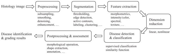
Computer assisted diagnosis flowchart.

3.1. Image preprocessing

As discussed in Section 2, current high resolution histology imaging technologies allow very high throughput production of high content images. Keeping up with the demands to produce diagnoses for such large quantities of very big and complex images is a significant challenge for the histopathology community. To process such images with CAD systems, image preprocessing can be applied to reduce the computational cost through multi-scale image decomposition such as subsampling or wavelet transform [53]. Then the low resolution images obtained this way can be first analyzed to roughly locate the regions of interest, and only these regions go to the higher resolution processing step. In case of poor quality input, e.g. severe noise, low intensity contrast with weak edges, and intensity inhomogeneity, other preprocessing techniques such as image smoothing, denoising, and enhancement may be applied for image restoration. Image smoothing usually refers to spatial filtering to highlight the major image structure by removing image noise and fine details, such as Gaussian filtering [53] and bilateral filtering [143]. Image denoising techniques are used to remove the noise introduced in the process of image acquisition, filtering, compression and reconstruction. Major categories of image denoising methods include partial differential equation (PDE)-based anisotropic diffusion [120], variational methods [129], robust statistics [12], and wavelet thresholding [39]. A review of current denoising methods is given in [4,151]. Image enhancement [53] is used to increase the contrast between the foreground (objects of interest) and background. Traditional enhancement techniques include adaptive filters [53] and inverse anisotropic diffusions [49].

3.2. Image segmentation

Image segmentation extracts objects/regions of interest from the background; these objects and regions are the focus for further disease identification and classification. Early segmentation methods (which are still used) include thresholding, edge detection, and region growing [53]. Thresholding approaches [130,135] use a value (threshold) to separate objects from background; this value is typically based on image intensity or its transforms such as Fourier descriptors or wavelets. The threshold is usually identified to satisfy some constraints or to optimize certain objective functions. For example, the commonly used Otsu’s method finds the threshold to maximize the between-class variance [53,135]. For histology image segmentation, multithresholding approaches [53,95,130] are mostly used to extract objects of different classes, e.g. nuclei, cytoplasm, stroma, and background. Edge detection [53] applies spatial filters (e.g. Canny and Sobel filters) to analyze neighboring pixel intensity or gradient differences to determine the border among objects and background. Postprocessing such as edge linking [53] is needed to remove spurious edges and connect broken edge segments to form meaningful boundaries. Region growing [53] groups pixels of similar features (e.g. intensity or texture) into connected areas, each of which is regarded homogenous or smooth according to predefined feature similarities. In recent years, with basic ideas from these previous low level segmentation techniques, more advanced algorithms have been proposed for better performance, including clustering-based techniques [11,44], and active contours [25,64,77,97,147]. For clustering-based methods, when prior knowledge of objects such as training samples or the number of clusters is available, supervised algorithms can be applied to build the classifier, which include artificial neural network, boosting approaches (e.g. AdaBoost [148]), support vector machine (SVM), and decision trees. In addition, Bayesian model-based approaches such as Markov random field (MRF) [105,106], hidden Markov model (HMM) [44], and conditional random field (CRF) [88] are commonly used to label pixels with the constraints of local pixel distribution, e.g. Gibbs distribution. Without a set of labeled samples, unsupervised techniques, such as K-means, fuzzy c-means, ISODATA clustering, Meanshift [40], self-organizing map [63], and adaptive resonance theory [23], can be applied to group image points to different objects. In certain applications such as texture segmentation, feature extraction from the whole image may be applied before segmentation, which can provide more discriminative features for clustering algorithms than regular intensities and colors.

As introduced in Section 1, the direct application of existing radiology image segmentation methods to histology images may not be optimal due to their significantly different characteristics, such as complex object distributions, and noisy and inhomogeneous connective tissue constituents in the stroma or epithelium region. To better understand these challenges, in this section we review the principles of currently commonly used image segmentation methods, including multithresholding [53], clustering-based methods (K-means [44] and mean shift [40]), and state-of-the-art methods using MRF [11,17,158] and active contours [27,93].

3.2.1. Multithresholding

Thresholding methods have been the most commonly used techniques for early image segmentation applications. As mentioned above, multilevel thresholding is necessary to extract different objects from histology images. For example, in the case of K object classes (s₁,s₂, …,s_K) in a digital image I (size X × Y), Otsu’s method finds the thresholds that maximizing the between-class variance

$${\sigma }_B^2=\sum _{k=1}^K{P}_k({\mu }_k-{\mu }_G)$$ (1)

where P_k = Σ_{l ∈ sk} p_l and p_l is the normalized histogram (probability) of intensity l, i.e. p_l = n_l/XY and n_l is the number of pixels with intensity l. μ_k is the current mean of s_k, μ_k = (1/P_k) Σ_{i ∈ sk} lp_l, and μ_G is the whole image intensity mean. The K classes are separated by K − 1 thresholds that maximize ${\sigma }_B^2$.

3.2.2. Clustering

In this section we introduce the segmentation implemented by two clustering methods: the traditional K-means clustering and a recent nonparametric algorithm, mean shift [40] clustering. K-means clustering groups image points into K clusters by minimizing the objective function

$$\sum _{k=1}^K\sum _{i\in s_k}{\mid I_i-{\mu }_k\mid }^2$$ (2)

where I_i is the intensity of the image point x_i in the class s_k.

Unlike K-means clustering, the mean shift algorithm does not assume prior knowledge of the number of clusters. For image segmentation, the image points in a d-dimensional (d = 3 for color image) feature space can be characterized by certain probability density function where dense regions correspond to the local maxima (modes) of the underlying distribution. Image points associated to the same mode (by a gradient ascent procedure) are grouped into one cluster. Notionally, the kernel density estimator for n points (x_i, i = 1,2,…,n) is defined as

$$f(x)=\frac{1}{{nh}^d}\sum _{i=1}^{n}K\left(\frac{\mathbf{x}-{\mathbf{x}}_i}{h}\right),$$ (3)

where K(x) is the kernel with the bandwidth h. In practice, radially symmetric kernels such as Epanechnikov and Gaussian kernels are usually used for clustering. The gradient ascent procedure is guaranteed to converge to a point where ∇f(x) = 0, i.e., a local maximum (mode).

3.2.3. Bayesian segmentation with MRF

When certain a priori knowledge of image intensity distribution is available, the image segmentation problem can be formulated as a maximum a posterior estimation with Bayesian model. In principle, given the observed image I, the objective is to label image pixels to different classes (S = {s₁,s₂,…,s_K}), which maximize the posterior probability of the labeling configuration F given the observation I

$$P(F\mid I)=\frac{P(I\mid F)P(F)}{P(I)}\propto P(I\mid F)P(F)$$ (4)

Because the density function P(I) is a factor to ensure the total probability is one, it can be omitted so that P(F|I) is proportional to the product of the likelihood P(I|F) and the prior probability P(F). The likelihood function characterizes the intensity distributions in different image regions, e.g. Gaussian distributions $P(I\mid F=s_k)=N(I\mid {\mu }_k,{\sigma }_k^2)$, where μk and ${\sigma }_k^2$ are the mean and variance of the class s_k. With MRF models, the prior probability P(F) is constructed on a small neighborhood system for a low computational cost. A MRF model maps a random field (F) to an image (I) in which each pixel is a random variable with all possible labels. According to the Hammersley–Clifford theorem [16], F is an MRF for I if and only if the prior probability is a Gibbs distribution with respect to the neighborhood system, P(F) = (1/Z)exp(−U(F)), where Z is a normalizing constant, and β is a positive constant that controls the interaction between point labels. U(F) is referred to as Gibbs energy which describes the a priori knowledge of interactions between labels assigned to neighboring points, e.g. different labels of neighboring points produce a large energy.

In practice the negative logarithm of the posterior probability is commonly used as the energy functional, which can be minimized by deterministic or stochastic approaches [11]. Compared with stochastic methods (e.g. Metropolis and Gibbs sampling algorithms [11]), in general deterministic algorithms such as iterated conditional modes (ICM) [11] and graph cuts [17] are more sensitive to the initial labeling, but are more computational efficient.

3.2.4. Active contours

Compared with above segmentation techniques, active contour models can achieve subpixel accuracy and always provide closed and smooth contours. Starting from the seminal work of Kass et al. [77] in the late 1980s, variations of the active contour models have been published, which can be categorized into two classes: snakes (also called explicit or parametric active contours) [33,103,157] and level set methods (also called implicit or geometric active contours) [25,27,97,147,149]. A review of recent active contours can be seen in [35,64,102]. In practice, level set methods are commonly used in situations where contour topology changes in deformation, which cannot be simply handled by snakes. Region information (e.g. intensity, color and texture descriptors) is usually used in level set methods [26,27,147,149] for more accurate results than edge-based models [25,97]; in these approaches, the image is usually segmented into multiple regions of interest with certain homogeneity constraints. In addition, region-based models are much less sensitive to contour initialization than edge-based models. Early region-based models, such as the Chan–Vese (CV) model [27], describe an image as a combination of piecewise constant regions that are separated by smooth curves. In [147], more advanced piecewise smooth models have been proposed to improve the performance of the CV model in the presence of intensity inhomogeneity. However, this model has a rather high computational cost. These early methods use global statistics and have difficulty extracting heterogeneous objects [91].

To improve the global model performance with respect to image intensity inhomogeneity, local region-based models [91,93] have been proposed. For example, in [93], a region-scalable fitting (RSF) energy is defined over the neighborhood of each image pixel, and the active contour is deformed to minimize the integration of the RSF energy across the entire image. However, the local models are still sensitive to the initial contour selection [70]. To overcome these disadvantages (and because we specifically seek a method for histology image segmentation), we have developed a localized K-means (LKM) energy to characterize the neighborhood class distributions of each pixel [68], which extends our recent local distribution fitting (LDF) model [70] to histology image segmentation. The LKM and LDF models enable a level set model to be used without initial contour specification, i.e., the level set function can be initialized with a constant instead of a distance function. Therefore, the proposed model improves the initialization sensitivity problem of most level set models. A detailed comparison of our LDF model and other local region-based models [91,93] can be seen in [70].

With recent progress on image segmentation, the above models have also been applied to microscopic image segmentation, such as mean shift clustering for cytology nuclei segmentation [15], MRF-based active contour for glandular boundary extraction [156], and active contours for histology image segmentation [37,62]. Specifically for histology image segmentation, we have developed two other models: Gaussian mixture model based pixel labeling [67] and color clustering [66], in addition to our active contour method [68]. These specialized models conduct multiple tissue segmentation by characterizing tissue distributions in histology images, which usually achieve better performance than the direct applications of classical image segmentation approaches.

3.3. Feature extraction and dimensionality reduction

Image feature extraction and selection is crucial for many image processing and computer vision applications, such as image retrieval [3,145], registration and matching [161], and pattern recognition [11,44]. For a CAD system, after image segmentation, image features are extracted from the regions of interest to detect and grade potential diseases. This is implemented by applying CAD systems to identify particular disease signatures with their image features. As introduced in Section 1, CAD systems for histology image analysis in general exploit a large number of features to derive clinically significant information. Traditional features [3,58,116,145,161] include morphometrics with object size and shape (e.g. compactness and regularities), topological or graph-based features (e.g. Voronoi diagrams, Delaunay triangulation, and minimum spanning trees), intensity and color features (e.g. statistics in different color spaces), and texture features (e.g. Haralick entropy, Gabor filter, power spectrum, co-occurrence matrices, and wavelets). In addition, besides using the image in the spatial domain, many features can also be extracted from other transformed spaces, e.g. frequency (Fourier) domain and wavelet transforms. Table 1 lists the major features employed by current CAD systems for carcinoma histology analysis.

Table 1.

Common image features for histology image analysis.

Morphometry	Area and size [1,48,75,87,105,106,108,121,131], boundary [109], shape (eccentricity, sphericity, elongation, compactness) [48,56,57,76,108,122]
Topological	Voronoi diagram [6,42,43,108,109], Delaunay triangulation [6,42,43,79], minimum spanning tree [6,42,43], skeleton [75]
Intensity/color	Color [41,109], intensity statistics [43]
Texture	Co-occurrence matrices [41,42,75], moments [75], Haralick and Gabor filter features [43], discrete texture, Markovian texture, run length texture [56,57,131], wavelets [41], density [121], Varma-Zisserman texton-based features [6], entropy [78]

With multiple classes of features extracted from large size histology images, the resulting vast quantity of data (e.g. a feature vector with thousands of elements for each pixel) can be prohibitive for feasible analysis, even with current high performance computing machines. Therefore, feature selection or dimensionality reduction (DR) schemes are necessary to determine the most discriminative features. Direct feature selection [137,152] is generally inefficient and suboptimal due to the large amount of features, especially for the blind selection (e.g. exhaustive search) without prior knowledge on individual feature discriminative capabilities. In addition, the general correlations among different features further impede effective feature selections. DR tools are commonly used to transform the feature points to a very low dimension space for a feasible selection and classification, including both linear and nonlinear techniques. A comparative study of major DR techniques can be seen in [92]. Linear techniques, such as principal component analysis (PCA) [36,44,142,160], linear discriminant analysis (LDA) [44], and multidimensional scaling (MDS) [146], are used in cases of linearly separable points in the feature space. These techniques assume Euclidean distance among the feature points. As an unsupervised data analysis tool, PCA finds orthogonal eigenvectors (i.e., principal components) along which the greatest amount of variability in the data lies. However, the projection of feature points to the principal component directions may not separate the data well for classification. In contrast, LDA is a supervised learning tool, which incorporates data label information to find the projections that maximize the ratio of the between-class variance and the within-class variance. MDS, on the other hand, reduces data dimensionality by preserving the least squares Euclidean distance in low-dimensional space. For nonlinear DR techniques such as spectral clustering [136], isometric mapping (Isomap) [140], locally linear embedding (LLE) [128], and Laplacian eigenmaps (LEM) [8], Euclidean relationship among feature points is not assumed. These techniques are more suitable for inherently nonlinear biomedical structures. Spectral clustering algorithms (graph embedding) employ graph theory to partition the graph (image) into clusters and separate them accordingly. The Isomap algorithm estimates geodesic distances among points along the manifold (i.e., a nonlinear surface embedded in the high-dimensional feature space along which dissimilarities between data points are best represented), and preserves the nonlinear geodesic distances (as opposed to Euclidean distances used in linear methods) while projecting the data onto a low-dimensional space. LLE uses weights to preserve local geometry in order to find the global nonlinear manifold structure of the data. Similar to the LLE, the LEM algorithm makes local connections but utilizes the Laplacian to simplify the determination of the locality preserving weights.

Based on the simplified feature vectors obtained by DR techniques, classification algorithms can be applied to identify diseases by comparing the input image features with a set of prederived training sample features. As in segmentation by clustering methods, supervised algorithms [11,44] can be applied to determine and grade disease. SVM [11], for example, which is one of the widely used machine learning tools, finds the hyperplane with maximum distances to the nearest training samples of different clusters. The original linear SVM can also be extended to nonlinear feature space with the Kernel Trick, i.e., kernel functions based on inner products of two feature vectors. In feature similarity computation, a number of metrics [3,11,44] can be applied besides the commonly used Euclidean distance, such as Mahalanobis and Chebyshev distances.

3.4. Postprocessing and results assessment

In practice, certain applications may require postprocessing for the CAD system results. For example, morphological operations such as dilation and erosion can be applied to remove spurious edges and obtain a smooth boundary (e.g. closing gaps in objects or separating connected objects) after thresholding [112]. For further advanced applications like image retrieval, the segmented object shapes may be stored as indexes to be matched with the user query. Similarly, image analysis results may be employed for image annotation and information integration.

After the cancer classification or grading, we can evaluate the performance of CAD systems by comparing their results with ground truth. As introduced in Section 1, unlike radiology image analysis applications, few ground truth data sets are available to evaluate the performance of histology image CAD systems. When a set of training data is available, we can divide the data set into two subsets and use one for training and the other one for testing. With the training subset, classifiers such as SVM are trained to learn the optimal parameter settings. Different schemes are used for accurate performance evaluation such as leave-one-out [137] or more general k-fold cross validation [159]. The grading results on the testing subset can be classified into one of the four categories: true positive (TP), false positive (FP), true negative (TN), and false negative (FN), based on which two performance indexes can be computed: sensitivity = number of TP/(number of TP + number of FN); specificity = number of TN/(number of TN + number of FP). Sensitivity measures the system accuracy in identifying the samples with the specific disease, and specificity measures the system accuracy in identifying the samples without the disease. Thus the higher the sensitivity and the specificity, the more accurate a CAD system is. A combination of the sensitivity and specificity is obtained as the area under a receiver operating characteristic (ROC) curve [119], which plots the sensitivity versus one minus the specificity and again, the larger the area, the better the system.

3.5. Microscopy image processing software

As stated in Section 1, while numerous image processing software systems have been developed for radiology and cytology applications, few systems target histology image analysis. Due to the specific imaging technologies and unique image characteristics of histology, most existing image processing systems cannot be applied directly to histology images. As one example, the open source cytology image analysis software, CellProfiler [90], is designed for biologists to quantitatively measure phenotypes in thousands of images automatically. The software is developed with Matlab^™, and all of the system functions are implemented by independent modules. For example, image segmentation can be implemented by configuring the ApplyThreshold or IdentifyPrimManual modules for manual segmentation, or using the IdentifyPrimAutomatic module for automatic segmentation. For automatic segmentation, five different thresholding methods are included in the module: Otsu’s method, the Mixture of Gaussian method, the Background method, the Robust Background method and the Ridler–Calvard method. Thus in practice, a specific application consists of a sequence of modules (a pipeline) to complete the task. This architecture allows the system flexibility in adapting to different tasks by selecting particular modules for the processing chain and setting their parameters for the particular task at hand.

Another important open source platform is Open Microscopy Environment (OME)⁵ [73,116,138], which is a software package and a set of standards for image informatics—the collection, maintenance, and analysis of biological images and the associated data. The aim of this system is to standardize how image information is stored, extracted and transported among different software applications, including both commercial and non-commercial products. OME is designed with standard client-server architecture. Fig. 4 shows the system architecture of the OMEv1.0 (Fig. 2 of [138]), in which client desktops are connected to an Oracle or PostgreSQL database through a middle layer that consists of a variety of applications, including import and export routines, data analysis and visualization tools, and other ancillary software. These applications enable users to access images by queries of content and meaning. For example, the Importer/Exporter provides interfaces to input images from other environments and save them in an OME XML file for output conforming to public web-compliant standards. The XML file format is defined to save the input images in a standard format for simple transport and storage, which follows the OME data model that consists of three parts: binary image data, metadata, and data type semantics. Image and data analysis are implemented by the analysis chain modules in the Analysis Subsystem.

Fig. 4.

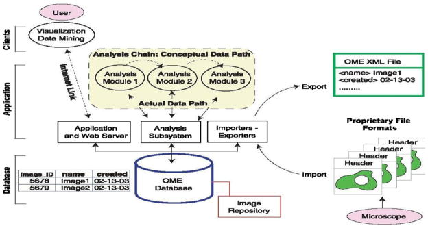
OME system architecture. (From [138]. Reprinted with permission from AAAS.)

In the current version of OME 2.6.x [139], the applications in the middle layer have been grouped into two modules: an image server (OMEIS) and a data server (OMEDS). OMEIS is an interface to a repository where image pixels, original image files, and other large binary objects are stored. OMEDS stores all meta-data and the derived knowledge about the images in a database. These servers are accessed using a web user interface via a Java API (web client), or by using a plugin for ImageJ (Java client) [73]. The major task of OME is not to create novel image analysis algorithms, but instead to develop of a structure that allows applications to access and use any data associated with, or generated from, digital microscope images. With this said, OME does provide a powerful image processing package, WND-CHARM [116,117], which extracts 1025 image features of intensity, texture, structure and objects from the image and its wavelet, Fourier, and Chebyshev transforms. Based on these features, region and image classification can be conducted for annotation. Both CellProfiler and OME work well on cytology images with separated cells and clear background, but have difficulties for histology image processing. For example, with the traditional thresholding methods included in the image segmentation modules, CellProfiler produces results similar to standard multithresholding or K-means clustering, which is not as accurate as the histology-oriented segmentation algorithms.

4. Carcinoma detection, grading, and CAD

In this section we describe detection, grading, and CAD systems for four carcinoma types: cervix [56,57,76,79,122], prostate [41,42,105,106,108], breast [6,43,109], and lung [75,78,87,131].

4.1. Cervix carcinoma histology analysis

Cervical carcinoma refers to cancer forming tissues of the uterine cervix, and is believed to be almost always caused by human papillomavirus (HPV) infection. Before the introduction of Pap testing and colposcopic examination in 1950s, it was a major cause of cancer death for American women. Since then, the death rate from cervical cancer has been significantly reduced.^6,7 This screening procedure can detect early cervical disease, based on which appropriate treatment such as Loop electrosurgical excision, cryotherapy, or laser ablation can be applied. Early cervical epithelial abnormalities are termed carcinoma in situ (CIS) [20] or dysplasia [125] that is further graded as mild, moderate, or severe degree [22,133]. To make the standard nomenclature more rigorous and consistent [22], a single diagnostic category was introduced in 1968, namely cervical intraepithelial neoplasia (CIN) [126]. CIN is divided into grades 1, 2 and 3, which correspond to mild dysplasia, moderate dysplasia, and severe dysplasia/CIS, respectively. In practice, final diagnosis of CIN is conducted not by Pap test, but by histopathology analysis of cervix tissues. CIN severity is based on the proportion of the epithelium with abnormal cells. For example, atypical cells are seen mostly in the lower third of the epithelium for CIN 1, lower half or two thirds of the epithelium for CIN 2, and full thickness of the epithelium for CIN 3. Fig. 5 shows H & E stained examples of normal, CIN 1, 2, and 3 histology images.

Fig. 5.

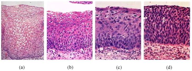
CIN examples: (a) normal; (b) CIN 1; (c) CIN 2; (d) CIN 3.

These images were published in “Robbins & Cotran Pathologic Basis of Disease”, Vinay Kumar, Abul Abbas, Nelson Fausto, and Jon Aster, Chapter 22 The Female Genital Tract, Figure 22–17 Spectrum of cervical intraepithelial neoplasia, p. 1020, Copyright Elsevier (2009).

To address the problem of large intra- and inter-pathologist variations in CIN grading, CAD systems [56,57,79,122] have been developed with the goal of providing unbiased and reproducible grading. The machine vision system in [79] automatically scores an input histology image for CIN degree. After thresholding to locate all nuclei, morphological features are computed to determine the CIN grade. 18 features are derived and LDA is applied to differentiate (a) normal and CIN 3, (b) koilocytosis and CIN 1, and (c) all CIN cases. The classification of normal versus CIN 3 achieves the best result (98.7%). In [56], about 120 morphometric and texture features are used for similar classification experiments. In [122], a Bayesian belief network is used to construct a decision support system to automatically determine the CIN grades. The Bayesian belief network consists of 8 histological features that are independently linked to a common decision node by a conditional probability matrix. The membership functions are used to derive the probabilities (likelihood) of alternative feature outcomes, based on which the diagnostic belief is computed for the decision of normal, koilocytosis, and CIN 1, 2, 3 grades.

4.2. Prostate carcinoma histology analysis

Prostate carcinoma refers to cancer forming in male prostate tissues, and is the second most common type of cancer among American men.^8,9 Annually there are more than 186,000 men in the U.S. diagnosed with prostate cancer and over 43,000 deaths [106]. Since the late 1980s, the overall death rate from prostate cancer has been significantly reduced, and in 2004, the estimated number of prostate cancer survivors was about two million in the U.S. This improved state for prostate health may reasonably be attributed to early detection and treatment, in particular by use of prostate-specific antigen (PSA) testing. Treatments include prostatectomy (surgery), chemotherapy, hormone therapy, and radiation therapy.¹⁰

Currently, visual analysis of prostate tissue samples remains the gold standard for cancer diagnosis. The Gleason grading scheme [50] is commonly used to grade the degree of malignancy on a scale of 1 (well differentiated glands) to 5 (poorly differentiated glands). The Gleason grades are determined by tissue characteristics such as the size and shape variations of nuclei and gland structures. Fig. 6 shows Dr. Gleason’s own annotated drawing of the five grades. Two major tissue patterns are usually selected from the specimen, and a Gleason grade is assigned to each one. An overall Gleason score is computed as a sum of these two grades, with a range from 2 to 10.

Fig. 6.

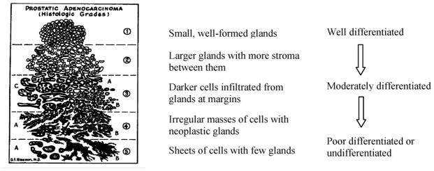
Gleason’s grades for prostate cancer.

To obtain higher sensitivity and better performance than previous methods in prostate cancer detection, a variation of MRF [106] replaces the commonly used potential functions (i.e. Gibbs distributions) with probability distributions. An automated detection method is proposed in [41], which employs the AdaBoost algorithm to combine the most discriminative features in a multi-scale way. After the detection step, researchers have applied machine learning and pattern classification techniques, such as SVM [42,108] and MRF [105], for automated grading.

4.3. Breast carcinoma histology analysis

Breast carcinoma includes cancers such as ductal or lobular carcinoma. Except for skin cancer, breast cancer is the most commonly diagnosed cancer for women in the U.S.^11,12 Each year more than 192,000 American women are diagnosed with breast cancer; about 90% of these will survive for at least 5 years. Regular mammographic examination for early detection is crucial for mortality reduction. For early stage treatment, mastectomy has now been replaced by breast-conserving surgery (lumpectomy) followed by local radiotherapy. Other treatments include combinations of chemotherapy and hormonal therapy.

In the U.S., breast cancer is classified by the Bloom–Richardson (BR) grading scheme [13],¹³ which includes low grade (nearly normal, well differentiated, slowly growing cells), intermediate grade (semi-normal, moderately differentiated cells), and high grade (abnormal, poorly differentiated, fast growing cells). The BR grade is based on three features: the proportion of tumor forming tubular structure; tumor mitotic degree (cell division rate); the regularity and uniformity of cell nuclei size and shape. A score of 1 (nearly normal) to 3 (high malignancy) is assigned to each feature. For example, >75% tumor cells in tubules is assigned a value of 1 for the first feature; a value of 2 is assigned to the second feature when the number of mitoses is between 10 and 20 in 10 high power fields; irregular large cell nuclei with multiple nucleoli is assigned a value of 3 for the third feature. The sum of the three scores results in a range of 3–9, which maps to the BR grading scheme, i.e. 3–5 for low grade, 6–7 for intermediate grade, and 8–9 for high grade. Fig. 7 shows histology examples of normal and three BR grades.

Fig. 7.

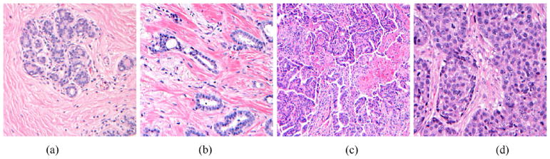
Breast carcinoma histology examples: (a) normal; (b) grade 1; (c) grade 2; (d) grade 3.

Illustration courtesy of Meenakshi Singh, MD, Department of Pathology, Stony Brook University Medical Center.

Existing CAD systems [1,6,21,43,109,121] for breast carcinoma detection and grading follow the common flowchart in Fig. 3. In [121], after cell nuclei detection, nine morphology and texture features are computed. The two most discriminative features are identified for degree classification. Four classifiers (linear, quadratic, neural network, and decision tree) are tested, with the quadratic classifier achieving minimum error. Similarly, in other CAD systems [1,6,109], after image segmentation to extract the regions of interest, a variety of features are computed, for example, area histograms [1], gland boundary features [109], graph-based features [6,43,109], and textural features [6,43]. The features extracted by these CAD systems are generally of large quantity (e.g. 1050 “bins” in [1] and over 3400 features in [43]), and because of this large size, they cannot be fed into the classifiers directly. Therefore, DR techniques (e.g. PCA [109] or graph embedding [43]) are usually applied to identify the most discriminative features. The reduced data is then fed to supervised classification tools such as SVM [1,6,43,109] for carcinoma detection and grading. For the specific case of nuclei segmentation in breast cancer tissues, [21] has a processing pipeline that includes preprocessing, watershed-based region growing for segmentation, and postprocessing for final shape extraction. A review of morphometric image analysis for breast cancer diagnosis is given in [48].

4.4. Lung carcinoma histology analysis

Lung carcinoma refers to the cancer forming in lung tissues, and is the third most common cancer for both men and women in the U.S.^14,15 Lung cancer causes more deaths for both men and women than any other cancers, which accounts for 29% of all cancer deaths in the U.S.¹⁶ Screening is generally done by chest X-ray. Treatment includes surgery, chemotherapy, and radiotherapy. Comprehensive and accurate lung tumor classification is required for selection of the appropriate treatment protocol.

Since the initial classification of lung cancer into four histological groups (i.e., squamous carcinoma, adenocarcinoma, and small and large cell undifferentiated carcinoma) in 1924 [89], a variety of standards have been proposed, including the World Health Organization (WHO) classifications of 1967 [153], 1981 [85], 1999 [141], and 2004 [154], the classification of the Veterans Administration Lung Cancer Chemotherapy Study Group (VALG) [101], the classification of the Working Party for Therapy of Lung Cancer (WP-L) [101], and that in the Armed Forces Institute of Pathology Fascicle by Carter and Eggleston [24]. Due to the rather complex tumor variations, current lung carcinoma classifications are usually organized with a hierarchical structure, i.e., main headings are followed by subtypes. The above classifications differ significantly in the organization of cases, even between the main groups [89]. For a practical application, it is important to select the classification that provides the most reproducible results for diagnosis. For example, the WHO classification of 2004 is currently widely accepted by clinicians and pathologists. This classification mainly uses two groups of carcinomas: small cell lung carcinoma and non-small cell carcinoma (i.e., adenocarcinoma, squamous carcinoma, and large cell carcinoma). Fig. 8 shows examples of these principal lung carcinomas.

Fig. 8.

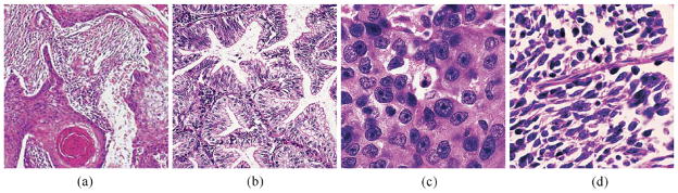
Lung carcinoma histology examples: (a) squamous cell carcinoma; (b) adenocarcinoma; (c) large cell carcinoma; (d) small cell carcinoma.

Figure (a) was published in “Pathology of the Lungs”, Bryan Corrin and Andrew G. Nicholson, Chapter 12 Tumors, Fig. 12.1.13 Squamous cell carcinoma, p. 543, Copyright Elsevier (2005). Figures (b)–(d) were published in “Rosai and Ackerman’s Surgical Pathology”, Juan Rosai, Chapter 7 Respiratory Tract, Fig. 7.129 Adenocarcinoma, p. 392, Fig. 7.131 Large cell carcinoma, p. 393, and Fig. 7.143 Small Cell Carcinoma, p. 399, Copyright Elsevier (2004).

Lung carcinoma histological diagnoses, like those for cancers in other tissues, may have significant intra- and inter-pathologist variations. CAD systems [75,78,87,131] attempt to improve on this variability for reproducible assessments. A training image set is constructed in [78] for different histological classes, and nine texture and morphometry features are used to compare test images with the training set for classification of tumor and non-tumor cases. In [131], four most discriminative features are selected from 114 texture features using LDA. These features describe the granularity and compactness of nuclear chromatin. The effectiveness of the selected features was evaluated by classifying lung carcinomas, specifically for neuroendocrine tumors. The authors argue that morphological features are not sufficient for discrimination of neuroendocrine tumors and, instead, that mitotic counts and presence of necrosis should be used for classification. In [87], five morphometric features were used for malignancy assessment of lung squamous carcinoma. A prognostic index was constructed, based on the mean nuclear volume. This index provides a functional tool for separating prognostically poor from prognostically favorable cases, and for predicting the 5-year survival rate. In [75], chromatin texture, morphological and densitometrical features are applied for neuroendocrine tumor classification. For survival analysis, five chromatin features were selected to construct the Cox variable [9].

Though histology image analysis provides a potent tool for lung carcinoma classification, it usually focuses on main headings with relatively clear cases. This is not sufficient for the more challenging subtype classification, especially for the new categories like neuroendocrine lung tumors [75]. In addition, lung cancers usually show histological heterogeneity, i.e., mixed cell types in different sections of the same tumor, which pose a significant challenge for histology image analysis. To address these issues, more fundamental and accurate knowledge at the molecular level, such as gene expression profiles [7,10,54] or proteomic signatures [132], are usually applied for a finer, hierarchical classification. Microarray methods are frequently used to find effective prognosis markers at the molecular level. Machine learning techniques including hierarchical clustering, SVM, and LDA, are used to analyze gene, chromatin, or protein for lung carcinoma classification and survival analysis. For the four carcinomas, Table 2 summarizes the early diagnosis and treatment methods, commonly used grading features and standards, and main machine learning and pattern classification techniques used by current CAD systems.

Table 2.

Diagnosis, grading, and algorithms for the four carcinomas.

	Early diagnosis and treatments	Grading standard	Features for grading	Learning tools and classifiers for CAD systems
Cervix	Pap test and colposcopic examination; Loop electrosurgical excision, cryotherapy, and ablation by laser heating	CIN: 1, 2, 3; TBS: LSIL, HSIL	Nuclear-cytoplasmic ratio in epithelium	LDA [56,57,79], Bayesian belief network [122]
Prostate	PSA test; prostatectomy, chemotherapy, hormone therapy, and radiation therapy	Gleason grading scheme: 1–5 (Gleason score: sum of two grades 2–10)	Size and shape distributions of nuclei and glands	MRF [105,106], AdaBoost [41], SVM [42,108], Bayesian classifier [108]
Breast	Mammographic screening; mastectomy, lumpectomy, chemotherapy, hormonal therapy	BR: low, intermediate, high (BR score: sum of three grades 3–9)	The proportion of tumor forming tubular structure; Tumor mitotic degree (cell division rate); The regularity and uniformity of cell nuclei size and shape.	LDA, forward & backward search, linear, quadratic, neural network, decision tree [121], PCA, Bayesian classifier, SVM [6,109], graph embedding, SVM [43], SVM [1]
Lung	Chest X-ray; surgery, chemotherapy, and radiotherapy	WHO 2004	Small cell lung carcinoma and non-small cell carcinoma (adenocarcinoma, squamous carcinoma, and large cell carcinoma)	LDA [54,131], PCA, SVM [132], K-Nearest Neighbor [10], hierarchical clustering [7]

5. Summary

Computer-based image analysis has become an increasingly important field because of the high rate of image production and the increasing reliance on these images by the biomedical community. This paper presents a survey for the application of histology image analysis to carcinoma detection and grading. Current histology technical procedures and imaging technologies to prepare tissue images were introduced in the beginning. We then reviewed the common processing steps of CAD systems, with a focus on image segmentation techniques. Specifically, nine commonly used approaches including mean shift clustering, Markov random field-based Bayesian segmentation, and level set models were presented as examples of state-of-the-art techniques, and their results are compared with those of traditional multithresholding and K-means clustering, as well as our three recent methods specifically designed for histology image segmentation. We provided both qualitative and quantitative comparison of these major approaches. We expect that this comparative study provides a concrete picture of the performance of currently available segmentation methods, and that our presentation is appropriate for readers in the computing and clinical communities.

In addition to the overview of CAD system functional modules, we also discussed practical histology applications and products. Four major carcinomas were selected to demonstrate the function of current computer assisted diagnosis systems, which help analyze the screening results to automatically determine the presence and malignancy of cancer. Compared with traditional medical image processing and analysis, histology image analysis is a new area with more challenging problems, and focuses on high throughput microscopic images with complex content and high resolution. A histology image usually has a much more complex structure than a radiological or a cytological one, with a number of objects of interest extensively distributed in the image. In addition, histology images are usually corrupted by noise and other gross structures, which result in spurious edges and blur boundaries for a rather difficult image segmentation and analysis. Most current CAD systems for histology image analysis are based on revising and adjusting existing image processing techniques (for radiology or cytology images) for the new applications, which may not be optimal for histology image processing requirements. Moreover, these systems usually use a set of heuristic procedures, which are empirically determined for specific applications. This significantly restricts the application of a CAD system for more general cases. A potential solution to address these difficulties is to develop algorithms specifically for histopathology applications. For the histology image segmentation example presented in Section 3, we showed that our models, which target histology images, improve the performance of other generative models. Based on these segmentation results, we are currently constructing a CAD system for automated CIN detection and grading, which includes two steps of epithelium region detection in histology slides and automated CIN grading. In the first step, we apply color (hue) and texture (moments [53], Gabor [98] and Haar [148] descriptors, and local binary patterns [114]) features to train supervised classifiers such as AdaBoost [148], adaptive neural network [11], and support vector machine [11]. Manifold learning techniques, including PCA, MDS, Isomap, LLE, and LEM, are employed to reduce the feature dimensionality. With our current experiments on the National Cancer Institute (NCI) ALTS¹⁷ project, AdaBoost outperforms others with the hue and LBP features. From the detected epithelium regions, we are working on the second phase to extract the density features (e.g. Voronoi diagrams and Delaunay triangles) of the segmented nuclei, which will be applied to train the classifiers for CIN grading.

For other possible solutions addressing the above histology image analysis challenges, more sophisticated strategies may be further exploited, which may be implemented in two directions: (a) technology combinations to enhance current algorithm and system performance, e.g. hierarchical processing and multiple classifier combination [84]; and (b) information integration to combine more comprehensive information from different resources for more accurate diagnosis and prognosis, e.g. multi-feature integration [41] or multi-modal [30]/multi-stain [34] image registration. In summary, to develop histopathology CAD systems for successful cancer detection and grading, future works should address the following open problems in the field; these problems usually require a close and consistent collaboration of computer scientists, clinicians and pathologists.

• Lack of quantitative imaging measurements for image generation and processing. For example, the tissue preparation and image production, and annotation and labeling procedures need to be standardized for a common protocol that may be adopted and reproduced by different parties.

• Lack of algorithm reproducibility and generality. To date, although many systems have been developed, it is difficult to apply them to similar or related problems, e.g. it is not clear which particular feature or algorithm is suitable for a specific histology sub-domain. There is no good understanding, for example, of the extent to which algorithms developed for prostate image analysis are useful for analyzing images of the uterine cervix. Unless it becomes possible to develop more general algorithms, automated histology image analysis will remain highly compartmentalized and carried out by “islands” of research groups which do not benefit greatly from each other’s work.

• Lack of standards and ground truth as reference for algorithm validation and comparison. So far the community has not developed any reference data sets that may be used to validate and compare algorithms. This is a common shortcoming in evaluation of biomedical image processing techniques, but seems to be especially acute for histology. It is crucial to understand how large such data sets would need to be and what range of variations they would need to cover, e.g. different imaging modalities and cancers. Can the existing methods to estimate ground truth that have been established for radiology images, e.g. STAPLE [150], be applied to histological applications. In addition, how can the community construct publication standards for histology image data, like DICOM for radiology images and MIAME 2.0 for microarray data?

• Lack of software and tools to process large quantity of data sets. Although there are numerous well developed tools, such as ImageJ, to process single images, tools to process large data sets with very large size images (e.g. histology slides) are lacking. Collaborations between computer scientists and pathologists are necessary to process the results of large scale studies such as the NCI ALTS project. One under-explored area is looking at existing technology in other, non-biomedical scientific groups which deal with very large image data analysis; for example, this may include geo-imagery acquired from satellites. What are the main gaps existing tools have, such as the OME and CellProfiler?

• Lack of integration with other mature platforms, e.g. ITK/VTK. The ITK and VTK play an important role in facilitating research and development in medical imaging and image analysis. Microscopy imaging would benefit from a similar effort. The NIH funded project, FARsight,¹⁸ is the one of the first such efforts for the study of complex and dynamic tissue microenvironments that are imaged by current optical microscopes. Can ITK/VTK be extended to microscopy, and can FARsight and other histology analysis systems be integrated with ITK/VTK? In addition, emerging imaging annotation standards, such as the NCI’s Annotation Imaging Markup (AIM) should be investigated for possible use as an image information interchange system for histology.

• Finally, computing requirements for histology image analysis algorithms can be substantial, so much so, that they impact the number algorithmic alternatives that can be investigated. Cheap, high-performance computing hardware is becoming available in the form of graphical processing units (GPUs) that may be hosted on consumer-grade computers, and offer a possible solution for off-loading compute-intensive algorithms. The principal cost is not hardware, but the development of algorithms with the specialized architecture to execute efficiently on the hardware. If libraries of basic image processing functions are developed for these GPU systems, and a method of pipelining large volume image data is developed, we will have a potentially large step taken in the direction of overcoming the current obstacles in the computing time required for algorithmic experimentation on large collections of histology images.

References

- 1.Adiga U, Malladi R, Fernandez-Gonzalez R, de Solorzano CO. High-throughput analysis of multispectral images of breast cancer tissue. IEEE Transactions on Image Processing. 2006;15(8):2259–2268. doi: 10.1109/tip.2006.875205. [DOI] [PubMed] [Google Scholar]
- 2.Albe X, Cornu MB, Margules S, Bisconte JC. Software package for the quantitative image analysis of histological sections. Computers and Biomedical Research. 1985;18(4):313–333. doi: 10.1016/0010-4809(85)90011-4. [DOI] [PubMed] [Google Scholar]
- 3.Antani S, Kasturi R, Jain R. A survey on the use of pattern recognition methods for abstraction, indexing and retrieval of images and video. Pattern Recognition. 2002;35(4):945–965. [Google Scholar]
- 4.Aubert G, Kornprobst P. Mathematical Problems in Image Processing: Partial Differential Equations and the Calculus of Variations. Springer; 2006. pp. 59–127. [Google Scholar]
- 5.Bankman I, editor. Handbook of Medical Image Processing and Analysis. 2. Academic Press; 2008. [Google Scholar]
- 6.Basavanhally A, Agner S, Alexe G, Bhanot G, Ganesan S, Madabhushi A. Manifold learning with graph-based features for identifying extent of lymphocytic infiltration from high grade HER2+ breast cancer histology. Workshop on Microscopic Image Analysis with Applications in Biology; 2008. [Google Scholar]
- 7.Beer DG, Kardia SLR, Huang C, Giordano TJ, Levin AM, Misek DE, Lin L, Chen G, Gharib TG, Thomas DG, Lizyness ML, Kuick R, Hayasaka S, Taylor JMG, Iannettoni MD, Orringer MB, Hanash S. Gene-expression profiles predict survival of patients with lung adenocarcinoma. Nature Medicine. 2002;8(8):816–824. doi: 10.1038/nm733. [DOI] [PubMed] [Google Scholar]
- 8.Belkin M, Niyogi P. Laplacian eigenmaps for dimensionality reduction and data representation. Neural Computation. 2003;15(6):1373–1396. [Google Scholar]
- 9.Bewick V, Cheek L, Ball J. Statistics review 12: survival analysis. Critical Care. 2004;8(5):389–394. doi: 10.1186/cc2955. [DOI] [PMC free article] [PubMed] [Google Scholar]
- 10.Bhattacharjee A, Richards WG, Staunton J, Li C, Monti S, Vasa P, Ladd C, Beheshti J, Bueno R, Gillette M, Loda M, Weber G, Mark EJ, Lander ES, Wong W, Johnson BE, Golub TR, Sugarbaker DJ, Meyerson M. Classification of human lung carcinomas by mRNA expression profiling reveals distinct adenocarcinoma subclasses. Proceedings of the National Academy of Sciences of the United States of America. 2001;98(24):13790–13795. doi: 10.1073/pnas.191502998. [DOI] [PMC free article] [PubMed] [Google Scholar]
- 11.Bishop CM. Pattern Recognition and Machine Learning. Springer; 2006. [Google Scholar]
- 12.Black M, Sapiro G, Marimont D, Heeger D. Robust anisotropic diffusion. IEEE Transactions on Image Processing. 1998;7(3):421–432. doi: 10.1109/83.661192. [DOI] [PubMed] [Google Scholar]
- 13.Bloom HJ, Richardson WW. Histological grading and prognosis in breast cancer; a study of 1409 cases of which 359 have been followed for 15 years. British Journal of Cancer. 1957;11(3):359–377. doi: 10.1038/bjc.1957.43. [DOI] [PMC free article] [PubMed] [Google Scholar]
- 14.Blum A, Zalaudek I, Argenziano G. Digital image analysis for diagnosis of skin tumors. Seminars in Cutaneous Medicine and Surgery. 2008;27(1):11–15. doi: 10.1016/j.sder.2007.12.005. [DOI] [PubMed] [Google Scholar]
- 15.Bergmeir C, Silvente MG, López-Cuervo JE, Benítez JM. Segmentation of cervical cell images using mean-shift filtering and morphological operators. SPIE Medical Imaging. 2010:7623. [Google Scholar]
- 16.Besag J. Spatial interaction and the statistical analysis of lattice systems. Journal of the Royal Statistical Society Series B. 1974;36(2):192–236. [Google Scholar]
- 17.Boykov Y, Veksler L, Zabih R. Fast approximate energy minimization via graph cuts. IEEE Transactions on Pattern Analysis and Machine Intelligence. 1995;17(2):158–171. [Google Scholar]
- 18.Boucheron LE, Bi Z, Harvey NR, Manjunath B, Rimm DL. Utility of multispectral imaging for nuclear classification of routine histopathology imager. BMC Cell Biology. 2007;8(Suppl 1):S8. doi: 10.1186/1471-2121-8-S1-S8. [DOI] [PMC free article] [PubMed] [Google Scholar]
- 19.Brinkhuis M, Wijnaendts LCD, van der Linden JC, van Unnik AJM, Voûte PA, Baak JPA, Meijer CJLM. Peripheral primitive neuroectodermal tumour and extra-osseous Ewing’s sarcoma; a histological, immunohistochemical and DNA flow cytometric study. Virchows Archiv. 1995;425:611–616. doi: 10.1007/BF00199351. [DOI] [PubMed] [Google Scholar]
- 20.Broders AC. Carcinoma in situ contrasted with benign penetrating epithelium. Journal of American Medical Association. 1932;99(20):1670–1674. [Google Scholar]
- 21.Brook A, El-Yaniv R, Isler E, Kimmel R, Meir R, Peleg D. Technical report. Technion - Israel Institute of Technology; 2006. Breast cancer diagnosis from biopsy images using generic features and SVMs. [Google Scholar]
- 22.Buckley CH, Butler EB, Fox H. Cervical intraepithelial neoplasia. Journal of Clinical Pathology. 1982;35(1):1–13. doi: 10.1136/jcp.35.1.1. [DOI] [PMC free article] [PubMed] [Google Scholar]
- 23.Carpenter GA, Grossberg S. Adaptive resonance theory. In: Arbib MA, editor. The Handbook of Brain Theory and Neural Networks. 2. MIT Press; 2003. pp. 87–90. [Google Scholar]
- 24.Carter D, Eggleston JC. Tumours of the Lower Respiratory Tract (Atlas of Tumour Pathology 2nd Series) Armed Forces Institute of Pathology; Washington DC: 1980. [Google Scholar]
- 25.Caselles V, Kimmel R, Sapiro G. Geodesic active contours. International Journal of Computer Vision. 1997;22(1):61–79. [Google Scholar]
- 26.Chan TF, Sandberg B, Vese LA. Active contours without edges for vector-valued images. Journal of Visual Communication and Image Representation. 2000;11:130–141. [Google Scholar]
- 27.Chan TF, Vese LA. Active contour without edges. IEEE Transactions on Image Processing. 2001;10(2):266–277. doi: 10.1109/83.902291. [DOI] [PubMed] [Google Scholar]
- 28.Chandler D, Roberson RW. Bioimaging: Current Techniques in Light & Electron Microscopy. Jones & Bartlett Publishers; 2008. [Google Scholar]
- 29.Chang C. Hyperspectral Imaging: Techniques for Spectral Detection and Classification. Springer; 2003. [Google Scholar]
- 30.Chappelow J, Madabhushi A, Rosen M, Tomasezweski J, Feldman M. Multimodal image registration of ex vivo 4 Tesla prostate MRI with whole mount histology for cancer detection. SPIE Medical Imaging. 2007;6512:S1–S12. [Google Scholar]
- 31.Chen T, Zhang W, Good S, Zhou K, Comaniciu D. Automatic follicle quantification from 3D ultrasound data using global/local context with database guided segmentation. IEEE Intl. Conf. on Computer Vision; 2009. [Google Scholar]
- 32.Claridge E, Cotton S, Hall P, Moncrieff M. From colour to tissue histology: physics-based interpretation of images of pigmented skin lesions. Medical Image Analysis. 2003;7(4):489–502. doi: 10.1016/s1361-8415(03)00033-1. [DOI] [PubMed] [Google Scholar]
- 33.Cohen L. On active contour models and balloons. CVGIP: Image Understanding. 1991;52(2):211–218. [Google Scholar]
- 34.Cooper L, Sertel O, Kong J, Lozanski G, Huang K, Gurcan MN. Feature-based registration of histopathology images with different stains: an application for computerized follicular lymphoma prognosis. Computer Methods and Programs in Biomedicine. 2009;97(3):182–192. doi: 10.1016/j.cmpb.2009.04.012. [DOI] [PMC free article] [PubMed] [Google Scholar]
- 35.Cremers D, Rousson M, Deriche R. A review of statistical approaches to level set segmentation: integrating color, texture, motion and shape. International Journal of Computer Vision. 2007;72(2):195–215. [Google Scholar]
- 36.Dai JJ, Lieu L, Rocke D. Dimension reduction for classification with gene expression microarray data. Statistical Applications in Genetics and Molecular Biology. 2006;5(1):1–15. doi: 10.2202/1544-6115.1147. [DOI] [PubMed] [Google Scholar]
- 37.Degerman J, Faijerson J, Althoff K, Thorlin T, Rodriguez JH, Gustavsson T. A comparative study between level set and watershed image segmentation for tracking stem cells in time-lapse microscopy. Microscopic Image Analysis with Applications in Biology. 2006 [Google Scholar]
- 38.Diaspro A. Confocal and Two-Photon Microscopy: Foundations, Applications and Advances. Wiley-Liss; 2001. [Google Scholar]
- 39.Donoho DL. De-noising by soft thresholding. IEEE Transactions on Information Theory. 1995;41:613–627. [Google Scholar]
- 40.Comaniciu D, Meer P. Mean shift: a robust approach towards feature space analysis. IEEE Transactions on Pattern Analysis and Machine Intelligence. 2002;24(5):603–619. [Google Scholar]
- 41.Doyle S, Madabhushi A, Feldman M, Tomaszeweski J. A boosting cascade for automated detection of prostate cancer from digitized histology. 13th Intl. Conf. on Medical Image Computing and Computer Assisted Intervention; 2006. pp. 504–511. [DOI] [PubMed] [Google Scholar]
- 42.Doyle S, Hwang M, Shah K, Madabhushi A, Tomasezweski J, Feldman M. Automated grading of prostate cancer using architectural and textural image features. 4th IEEE International Symposium on Biomedical Imaging; 2007. pp. 1284–1287. [Google Scholar]
- 43.Doyle S, Agner S, Madabhushi A, Feldman M, Tomaszewski J. Automated grading of breast cancer histopathology using spectral clustering with textural and architectural image features. 5th IEEE International Symposium on Biomedical Imaging; 2008. pp. 496–499. [Google Scholar]
- 44.Duda RO, Hart PE, Stork DG. Pattern Classification. 2. Wiley; 2000. [Google Scholar]
- 45.Elston CW, Ellis IO. Pathological prognostic factors in breast cancer. I. The value of histological grade in breast cancer: experience from a large study with long-term follow-up. Histopathology. 1991;19:403–410. doi: 10.1111/j.1365-2559.1991.tb00229.x. [DOI] [PubMed] [Google Scholar]
- 46.Ganster H, Pinz A, Röhrer R, Wildling E, Binder M, Kittler H. Automated melanoma recognition. IEEE Transactions on Medical Imaging. 2001;20(3):233–239. doi: 10.1109/42.918473. [DOI] [PubMed] [Google Scholar]
- 47.Gartner LP, Hiatt JL. Color Textbook of Histology: With Student Consult Online Access. 3. Saunders; 2006. [Google Scholar]
- 48.Gil J, Wu H, Wang BY. Image analysis and morphometry in the diagnosis of breast cancer. Microscopy Research and Technique. 2002;59(2):109–118. doi: 10.1002/jemt.10182. [DOI] [PubMed] [Google Scholar]
- 49.Gilboa G, Sochen N, Zeevi Y. Forward-and-backward diffusion processes for adaptive image enhancement and denoising. IEEE Transactions on Image Processing. 2002;11(7):689–703. doi: 10.1109/TIP.2002.800883. [DOI] [PubMed] [Google Scholar]
- 50.Gleason DF. Classification of prostatic carcinomas. Cancer Chemotherapy Reports. 1966;50(3):125–128. [PubMed] [Google Scholar]
- 51.Glotsos D, Spyridonos P, Cavouras D, Ravazoula P, Dadioti PA, Nikiforidis G. Automated segmentation of routinely hematoxylin–eosin-stained microscopic images by combining support vector machine clustering and active contour models. Analytical and Quantitative Cytology and Histology. 2004;26(6):331–340. [PubMed] [Google Scholar]
- 52.Goldys EM. Fluorescence Applications in Biotechnology and Life Sciences. Wiley-Blackwell; 2009. [DOI] [PubMed] [Google Scholar]
- 53.Gonzalez RC, Woods RE. Digital Image Processing. 3. Pearson Prentice Hall; 2008. [Google Scholar]
- 54.Gordon GJ, Jensen RV, Hsiao L, Gullans SR, Blumenstock JE, Ramaswamy S, Richards WG, Sugarbaker DJ, Bueno R. Translation of microarray data into clinically relevant cancer diagnostic tests using gene expression ratios in lung cancer and mesothelioma. Cancer Research. 2002;62:4963–4967. [PubMed] [Google Scholar]
- 55.Greenberg SD, editor. Computer-Assisted Image Analysis Cytology. S. Karger AG; 1984. [Google Scholar]
- 56.Guillaud M, Cox D, Malpica A, Staerkel G, Matisic J, Niekirk DV, Adler-Storthz K, Poulin N, Follen M, MacAulay C. Quantitative histopathological analysis of cervical intra-epithelial neoplasia sections: methodological issues. Cellular Oncology. 2004;26:31–43. doi: 10.1155/2004/238769. [DOI] [PMC free article] [PubMed] [Google Scholar]
- 57.Guillaud M, Adler-Storthz K, Malpica A, Staerkel G, Matisic J, Niekirkd DV, Cox D, Poulina N, Follen M, MacAulaya C. Subvisual chromatin changes in cervical epithelium measured by texture image analysis and correlated with HPV. Gynecologic Oncology. 2005;99:S16–S23. doi: 10.1016/j.ygyno.2005.07.037. [DOI] [PubMed] [Google Scholar]
- 58.Gurevich IB, Koryabkina IV. Comparative analysis and classification of features for image models. Pattern Recognition and Image Analysis. 2006;16(3):265–297. [Google Scholar]
- 59.Guo AC, Cummings TJ, Dash RC, Provenzale JM. Lymphomas and high-grade astrocytomas: comparison of water diffusibility and histologic characteristics. Radiology. 2002;224(1):177–183. doi: 10.1148/radiol.2241010637. [DOI] [PubMed] [Google Scholar]
- 60.Gurcan M, Boucheron L, Can A, Madabhushi A, Rajpoot N, Yener B. Histopathological image analysis: a review. IEEE Reviews in Biomedical Engineering. 2009;2:147–171. doi: 10.1109/RBME.2009.2034865. [DOI] [PMC free article] [PubMed] [Google Scholar]
- 61.Gurcan MN, Pan T, Shimada H, Saltz J. Image analysis for neuroblastoma classification: segmentation of cell nuclei. 28th Annual Intl. Conf. of the IEEE Engineering in Medicine and Biology Society Conference; 2006. pp. 4844–4847. [DOI] [PubMed] [Google Scholar]
- 62.Hafiane A, Bunyak F, Palaniappan K. Level set-based histology image segmentation with region-based comparison. Microscopic Image Analysis with Applications in Biology. 2008 [Google Scholar]
- 63.Haykin S. Neural Networks—A Comprehensive Foundation. 2. Prentice-Hall; 1999. Self-organizing maps. [Google Scholar]
- 64.He L, Peng Z, Everding B, Wang X, Han C, Weiss K, Wee WG. A comparative study of deformable contour method in medical image segmentation. Image and Vision Computing. 2008;26(2):141–163. [Google Scholar]
- 65.He L. Towards Image Understanding: Deformable Contour and Graph-based Image Segmentation and Recognition. Lambert Academic Publishing; 2009. [Google Scholar]
- 66.He L, Long LR, Antani S, Thoma GR. Local and global Gaussian mixture models for hematoxylin and eosin stained histology image segmentation. IEEE 10th Intl. Conf. on Hybrid Intelligence Systems; 2010. [Google Scholar]
- 67.He L, Long LR, Antani S, Thoma GR. Distribution fitting-based pixel labeling for histology image segmentation. SPIE Medical Imaging, Computer-Aided Diagnosis Conference; 2011. [Google Scholar]
- 68.He L, Long LR, Antani S, Thoma GR. Multiphase level set model with local K-means energy for biomedical image segmentatio. IEEE Intl. Conf. Healthcare Informatics, Imaging, and Systems Biology; 2011. [Google Scholar]
- 69.He L, Long LR, Antani S, Thoma G. Computer Assisted Diagnosis in Histopathology. In: Zhao Z, editor. Sequence and Genome Analysis: Methods and Applications. iConcept Press; 2010. pp. 271–287. [Google Scholar]
- 70.He L, Zheng S, Wang L. Boundary extraction by level set integration of neighborhood-based distribution information. Journal of Visual Communication and Image Representation. 2010;21(4):343–354. [Google Scholar]
- 71.Herman B. Fluorescence Microscopy. 2. Garland Science; 1997. [Google Scholar]
- 72.Ibanez L, Schroeder W. The ITK Software Guide 2.4. Kitware; 2005. [Google Scholar]
- 73.Johnston J, Nagaraja A, Hochheiser H, Goldberg IG. A flexible framework for web interfaces to image databases: supporting user-defined ontologies and links to external databases. 3rd IEEE International Symposium on Biomedical Imaging; 2006. pp. 1380–1383. [Google Scholar]
- 74.Jungueira L, Carneiro J. Basic Histology: Text & Atlas. 11. McGraw-Hill Medical; 2005. [Google Scholar]
- 75.Jütting U, Gais P, Rodenacker K, Böhm J, Koch S, Präuer HW, Höfler H. Diagnosis and prognosis of neuroendocrine tumors of the lung by means of high resolution image analysis. Analytical Cell Pathology. 1999;18(2):109–119. doi: 10.1155/1999/695907. [DOI] [PMC free article] [PubMed] [Google Scholar]
- 76.Kalof AN, Cooper K. Our approach to squamous intraepithelial lesions of the uterine cervix. Journal of Clinical Pathology. 2007;60:449–455. doi: 10.1136/jcp.2005.036426. [DOI] [PMC free article] [PubMed] [Google Scholar]
- 77.Kass M, Witkin A, Terzopoulos D. Snakes: active contour models. International Journal of Computer Vision. 1988;1(4):321–331. [Google Scholar]
- 78.Kayser G, Riede U, Werner M, Hufnagl P, Kayser K. Towards an automated morphological classification of histological images of common lung carcinomas. Electronic Journal of Pathology and Histology. 2002;8(2):22–30. [Google Scholar]
- 79.Keenan SJ, Diamond J, McCluggage WG, Bharucha H, Thompson D, Bartels PH, Hamilton PW. An automated machine vision system for the histological grading of cervical intraepithelial neoplasia (CIN) Journal of Pathology. 2000;192(3):351–362. doi: 10.1002/1096-9896(2000)9999:9999<::AID-PATH708>3.0.CO;2-I. [DOI] [PubMed] [Google Scholar]
- 80.Kiernan JA. Histological and Histochemical Methods: Theory and Practice. 4. Cold Spring Harbor Laboratory Press; 2008. [Google Scholar]
- 81.Kong J, Shimada H, Boyer K, Saltz J, Gurcan MN. Image analysis for automated assessment of grade of neuroblastic differentiation. 4th IEEE International Symposium on Biomedical Imaging; 2007. pp. 61–64. [Google Scholar]
- 82.Kong J, Sertel O, Lozanski G, Boyer K, Saltz J, Gurcan MN. Automated detection of follicular centers for follicular lymphoma grading. Advancing Practice, Instruction, and Innovation Through Informatics Conference; 2007. [Google Scholar]
- 83.Kong J, Sertel O, Shimada H, Boyer K, Saltz J, Gurcan MN. A multi-resolution image analysis system for computer-assisted grading of neuroblastoma differentiation. SPIE Medical Imaging. 2008;6915:69151T.1–69151T.11. [Google Scholar]
- 84.Kong J, Sertel O, Shimada H, Boyer KL, Saltz JH, Gurcan MN. Computer-aided evaluation of neuroblastoma on whole-slide histology images: classifying grade of neuroblastic differentiation. Pattern Recognition. 2009;42(6):1080–1092. doi: 10.1016/j.patcog.2008.10.035. [DOI] [PMC free article] [PubMed] [Google Scholar]
- 85.Kreyberg L, Liebow AA, Uehlinger EA. Histological Typing of Lung Tumours. 2. WHO; Geneva: 1981. [Google Scholar]
- 86.Kuo J. Electron Microscopy: Methods and Protocols (Methods in Molecular Biology) 2. Humana Press; 2007. [Google Scholar]
- 87.Ladekarl M, Boek-Hansen T, Henrik-Nielsen R, Mourifzen C, Henriques U, Sørensen FB. Objective malignancy grading of squamous cell carcinoma of the lung: stereologic estimates of mean nuclear size are of prognostic value, independent of clinical stage of disease. Cancer. 1995;76(5):797–802. doi: 10.1002/1097-0142(19950901)76:5<797::aid-cncr2820760513>3.0.co;2-m. [DOI] [PubMed] [Google Scholar]
- 88.Lafferty J, McCallum A, Pereira F. Conditional random fields: probabilistic models for segmenting and labeling sequence data. 18th Intl. Conf. on Machine Learning; 2001. pp. 282–289. [Google Scholar]
- 89.Lamb D. Histological classification of lung cancer. Thorax. 1984;39:161–165. doi: 10.1136/thx.39.3.161. [DOI] [PMC free article] [PubMed] [Google Scholar]
- 90.Lamprecht MR, Sabatini DM, Carpenter AE. CellProfiler: free, versatile software for automated biological image analysis. Biotechniques. 2007;42(1):71–75. doi: 10.2144/000112257. [DOI] [PubMed] [Google Scholar]
- 91.Lankton S, Tannenbaum A. Localizing region-based active contours. IEEE Transactions on Image Processing. 2008;17(11):2029–2039. doi: 10.1109/TIP.2008.2004611. [DOI] [PMC free article] [PubMed] [Google Scholar]
- 92.Lee G, Rodriguez C, Madabhushi A. Investigating the efficacy of nonlinear dimensionality reduction schemes in classifying gene and protein expression studies. IEEE/ACM Transactions on Computational Biology and Bioinformatics. 2008;5(3):368–384. doi: 10.1109/TCBB.2008.36. [DOI] [PMC free article] [PubMed] [Google Scholar]
- 93.Li C, Kao C, Gore J, Ding Z. Minimization of region-scalable fitting energy for image segmentation. IEEE Transactions on Image Processing. 2008;17(10):1940–1949. doi: 10.1109/TIP.2008.2002304. [DOI] [PMC free article] [PubMed] [Google Scholar]
- 94.Lichtman JW, Conchello J. Fluorescence microscopy. Nature Methods. 2005;2(12):910–919. doi: 10.1038/nmeth817. [DOI] [PubMed] [Google Scholar]
- 95.Loukas CG, Linney A. A survey on histological image analysis-based assessment of three major biological factors influencing radiotherapy: proliferation, hypoxia and vasculature. Computer Methods and Programs in Biomedicine. 2004;74(3):183–199. doi: 10.1016/j.cmpb.2003.07.001. [DOI] [PubMed] [Google Scholar]
- 96.Mainen ZF, Maletic-Savatic M, Shi SH, Hayashi Y, Malinow R, Svoboda K. Two-photon imaging in living brain slices. Methods. 1999;18(2):231–239. doi: 10.1006/meth.1999.0776. [DOI] [PubMed] [Google Scholar]
- 97.Malladi R, Sethian J, Vemuri B. Shape modeling with front propagation. IEEE Transactions on Pattern Analysis and Machine Intelligence. 1995;17(2):158–171. [Google Scholar]
- 98.Manjunath BS, Ma WY. Texture features for browsing and retrieval of image data. IEEE Transactions on Pattern Analysis and Machine Intelligence. 1996;18(8):837–842. [Google Scholar]
- 99.Mankin HJ, Hornicek FJ. Diagnosis classification, and management of soft tissue sarcomas. Cancer Control. 2005;12(1):5–21. doi: 10.1177/107327480501200102. [DOI] [PubMed] [Google Scholar]
- 100.Masood K, Rajpoot N. Texture based classification of hyperspectral colon biopsy samples using CBLP. International Symposium on Biomedical Imaging; 2009. pp. 1284–1287. [Google Scholar]
- 101.Mathews MJ. Problems in morphology and behaviour of broncho-pulmonary malignant disease. In: Israel L, Chahinian P, editors. Lung Cancer-Natural History, Prognosis and Therapy. Academic Press; 1976. pp. 23–63. [Google Scholar]
- 102.McInerney T, Terzopoulos D. Deformable models in medical image analysis: a survey. Medical Image Analysis. 1996;1(2):91–108. doi: 10.1016/s1361-8415(96)80007-7. [DOI] [PubMed] [Google Scholar]
- 103.McInerney T, Terzopoulos D. T-Snakes: topologically adaptive snakes. Medical Image Analysis. 2000;4:73–91. doi: 10.1016/s1361-8415(00)00008-6. [DOI] [PubMed] [Google Scholar]
- 104.Mills SE. Histology for Pathologists. 3. Lippincott Williams & Wilkins; 2006. [Google Scholar]
- 105.Monaco J, Tomaszewski J, Feldman M, Moradi M, Mousavi P, Boag A, Davidson C, Abolmaesumi P, Madabhushi A. Detection of prostate cancer from whole-mount histology images using Markov random fields. Workshop on Microscopic Image Analysis with Applications in Biology; 2008. [Google Scholar]
- 106.Monaco J, Tomaszewski J, Feldman M, Mehdi M, Mousavi P, Boag A, Davidson C, Abolmaesumi P, Madabhushi A. Probabilistic pair-wise Markov models: application to prostate cancer detection. SPIE Medical Imaging. 2009;7259:725903-1–725903-12. [Google Scholar]
- 107.Murphy DB. Fundamentals of Light Microscopy and Electronic Imaging. Wiley-Liss; 2001. [Google Scholar]
- 108.Naik S, Doyle S, Madabhushi A, Tomaszewski J, Feldman M. Gland segmentation and Gleason grading of prostate histology by integrating low-, high-level and domain specific information. Workshop on Microscopic Image Analysis with Applications in Biology; 2007. [Google Scholar]
- 109.Naik S, Doyle S, Agner S, Madabhushi A, Feldman M, Tomaszewski J. Automated gland and nuclei segmentation for grading of prostate and breast cancer histopathology. 5th IEEE International Symposium on Biomedical Imaging; 2008. pp. 284–287. [Google Scholar]
- 110.Nattkemper TW. Automatic segmentation of digital micrographs: a survey. 11th World Congress on Medical Informatics; 2004. pp. 847–852. [PubMed] [Google Scholar]
- 111.Nelson DL, Cox MM. Lehninger Principles of Biochemistry. 4. W.H. Freeman; 2004. [Google Scholar]
- 112.Nedzved A, Ablameyko S, Pitas I. Morphological segmentation of histology cell images. Intl. Conf. on Pattern Recognition; 2000. pp. 500–503. [Google Scholar]
- 113.Oheim M, Michael DJ, Geisbauer M, Madsen D, Chow RH. Principles of two-photon excitation fluorescence microscopy and other nonlinear imaging approaches. Advanced Drug Delivery Reviews. 2006;58(7):788–808. doi: 10.1016/j.addr.2006.07.005. [DOI] [PubMed] [Google Scholar]
- 114.Ojala T, Pietikäinen M, Mäenpää T. Multiresolution gray-scale and rotation invariant texture classification with local binary patterns. IEEE Transactions on Pattern Analysis and Machine Intelligence. 2002;24(7):971–987. [Google Scholar]
- 115.Ong SH, Jin XC, Jayasooriah R. Sinniah, Image analysis of tissue sections. Computers in Biology and Medicine. 1996;26(3):269–279. doi: 10.1016/0010-4825(96)00004-2. [DOI] [PubMed] [Google Scholar]
- 116.Orlov N, Johnston J, Macura T, Shamir L, Goldberg I. Computer vision for microscopy applications. In: Obinata G, Dutta AV, editors. Vision Systems—Segmentation and Pattern Recognition. ARS Press; 2007. pp. 221–242. [Google Scholar]
- 117.Orlov N, Shamir L, Macura T, Johnston J, Eckley DM, Goldberg IG. WND-CHARM: multipurpose image classification using compound image transforms. Pattern Recognition Letter. 2008;29:1684–1693. doi: 10.1016/j.patrec.2008.04.013. [DOI] [PMC free article] [PubMed] [Google Scholar]
- 118.Pawley JB. Handbook of Biological Confocal Microscopy. 3. Springer; 2006. [Google Scholar]
- 119.Pepe MS. The Statistical Evaluation of Medical Tests for Classification and Prediction. Oxford University Press; 2004. [Google Scholar]
- 120.Perona P, Malik J. Scale-space and edge detection using anisotropic diffusion. IEEE Transactions on Pattern Analysis and Machine Intelligence. 1990;12(7):629–639. [Google Scholar]
- 121.Petushi S, Garcia FU, Haber MM, Katsinis C, Tozeren A. Large-scale computations on histology images reveal grade-differentiating parameters for breast cancer. BMC Medical Imaging. 2006;6(14) doi: 10.1186/1471-2342-6-14. [DOI] [PMC free article] [PubMed] [Google Scholar]
- 122.Price GJ, Mccluggage WG, Morrison ML, Mcclean G, Venkatraman L, Diamond J, Bharucha H, Montironi R, Bartels PH, Thompson D, Hamilton PW. Computerized diagnostic decision support system for the classification of preinvasive cervical squamous lesions. Human Pathology. 2003;34(11):1193–1203. doi: 10.1016/s0046-8177(03)00421-0. [DOI] [PubMed] [Google Scholar]
- 123.Radosevich AJ, Bouchard MB, Burgess SA, Chen BR, Hillman EMC. Hyperspectral in vivo two-photon microscopy of intrinsic contrast. Optics Letters. 2008;33(18):2164–2166. doi: 10.1364/ol.33.002164. [DOI] [PMC free article] [PubMed] [Google Scholar]
- 124.Ramjiawan B, Ariano RE, Mantsch HH, Maiti P, Jackson M. Immunofluorescence imaging as a tool for studying the pharmacokinetics of a human monoclonal single chain fragment antibody. IEEE Transactions on Medical Imaging. 2002;21(10):1317–1323. doi: 10.1109/TMI.2002.806275. [DOI] [PubMed] [Google Scholar]
- 125.Reagan JW, Seidermann IL, Saracusa Y. The cellular morphology of carcinoma in situ and dysplasia or atypical hyperplasia of the uterine cervix. Cancer. 1953;6:224–235. doi: 10.1002/1097-0142(195303)6:2<224::aid-cncr2820060203>3.0.co;2-h. [DOI] [PubMed] [Google Scholar]
- 126.Richart RM. Natural history of cervical intraepithelial neoplasia. Clinical Obstetrics and Gynecology. 1967;10(4):748–784. [Google Scholar]
- 127.Ross M, Kaye GI, Pawlina W. Histology: a Text and Atlas. 4. Lippincott Williams & Wilkins; 2002. [Google Scholar]
- 128.Roweis S, Saul L. Nonlinear dimensionality reduction by locally linear embedding. Science. 2000;290(5500):2323–2326. doi: 10.1126/science.290.5500.2323. [DOI] [PubMed] [Google Scholar]
- 129.Rudin L, Osher S, Fatemi E. Nonlinear total variation based noise removal algorithms. Physica D. 1992;60:259–268. [Google Scholar]
- 130.Sahoo PK, Soltani S, Wong AKC. Survey: a survey of thresholding techniques. Computer Vision Graphics Image Processing. 1988;41:233–260. [Google Scholar]
- 131.Schmid K, Angerstein N, Geleff S, Gschwendtner A. Quantitative nuclear texture features analysis confirms WHO classification 2004 for lung carcinomas. Modern Pathology. 2006;19:453–459. doi: 10.1038/modpathol.3800541. [DOI] [PubMed] [Google Scholar]
- 132.Seike M, Kondo T, Fujii K, Okano T, Yamada T, Matsuno Y, Gemma A, Kudoh S, Hirohashi S. Proteomic signatures for histological types of lung cancer. Proteomics. 2005;5:2939–2948. doi: 10.1002/pmic.200401166. [DOI] [PubMed] [Google Scholar]
- 133.Sellors JW, Sankaranarayanan R, editors. Colposcopy and Treatment of Cervical Intraepithelial Neoplasia: A Beginner’s Manual. IARC; 2003. [Google Scholar]
- 134.Sertel O, Kong J, Lozanski G, Catalyurek U, Saltz J, Gurcan MN. Computerized microscopic image analysis of follicular lymphoma. SPIE Medical Imaging. 2008;6915:6915-1–6915-11. [Google Scholar]
- 135.Sezgin M, Sankur B. Survey over image thresholding techniques and quantitative performance evaluation. Journal of Electronic Imaging. 2003;13(1):146–165. [Google Scholar]
- 136.Shi J, Malik J. Normalized cuts and image segmentation. IEEE Transactions on Pattern Analysis and Machine Intelligence. 2000;22(8):888–905. [Google Scholar]
- 137.Spyridonos P, Ravazoula P, Cavouras D, Berberidis K, Nikiforidis G. Computer-based grading of haematoxylin-eosin stained tissue sections of urinary bladder carcinomas. Medical Informatics and the Internet in Medicine. 2001;26(3):179–190. doi: 10.1080/14639230110065757. [DOI] [PubMed] [Google Scholar]
- 138.Swedlow JR, Goldberg IG, Brauner E, Sorger PK. Informatics and quantitative analysis in biological imaging. Science. 2003;300:100–102. doi: 10.1126/science.1082602. [DOI] [PMC free article] [PubMed] [Google Scholar]
- 139.Swedlow JR, Goldberg IG, Eliceiri KW. the OME Consortium, Bioimage informatics for experimental biology. Annual Review of Biophysics. 2009;38:327–346. doi: 10.1146/annurev.biophys.050708.133641. [DOI] [PMC free article] [PubMed] [Google Scholar]
- 140.Tenenbaum J, de Silva V, Langford JC. A global geometric framework for nonlinear dimensionality reduction. Science. 2000;290(5500):2319–2322. doi: 10.1126/science.290.5500.2319. [DOI] [PubMed] [Google Scholar]
- 141.Travis WD, Colby TV, Corrin B, Shimosato Y, Brambilla E, Sobin LH. Histological Typing of Lung and Pleural Tumours. 3. WHO; Geneva: 1999. [Google Scholar]
- 142.Truntzer C, Mercier C, Este‘ve J, Gautier C, Roy P. Importance of data structure in comparing two dimension reduction methods for classification of microarray gene expression data. BMC Bioinformatics. 2007;8(90) doi: 10.1186/1471-2105-8-90. [DOI] [PMC free article] [PubMed] [Google Scholar]
- 143.Tomasi C, Manduchi R. Bilateral filtering for gray and color images. IEEE Intl. Conf. Computer Vision; 1998. pp. 839–846. [Google Scholar]
- 144.Török P, Kao F. Optical Imaging and Microscopy. 2. Springer; 2007. [Google Scholar]
- 145.Veltkamp RC, Tanase M, Sent D. Features in content-based image retrieval systems: a survey. In: Veltkamp RC, Burkhardt H, Kriegel H-P, editors. State-of-the-Art in Content-Based Image and Video Retrieval. Kluwer Academic Publishers; 2001. pp. 97–124. [Google Scholar]
- 146.Venna J, Kaski S. Local multidimensional scaling. Neural Networks. 2006;19:889–899. doi: 10.1016/j.neunet.2006.05.014. [DOI] [PubMed] [Google Scholar]
- 147.Vese LA, Chan TF. A multiphase level set framework for image segmentation using the Mumford and Shah model. International Journal of Computer Vision. 2002;50(3):217–293. [Google Scholar]
- 148.Viola P, Jones M. Rapid object detection using a boosted cascade of simple features. IEEE Conference Computer Vision and Pattern Recognition; 2001. pp. 511–518. [Google Scholar]
- 149.Wang X, He L, Wee WG. Deformable contour method: a constrained optimization approach. International Journal of Computer Vision. 2004;59(1):87–108. [Google Scholar]
- 150.Warfield SK, Zou KH, Wells WM. Simultaneous truth and performance level estimation (STAPLE): an algorithm for the validation of image segmentation. IEEE Transactions on Medical Imaging. 2004;23(7):903–921. doi: 10.1109/TMI.2004.828354. [DOI] [PMC free article] [PubMed] [Google Scholar]
- 151.Weickert J. Anisotropic Diffusion in Image Processing. Teubner-Verlag; 1998. [Google Scholar]
- 152.Weyn B, Wouwer GV, Daele AV, Scheunders P, Dycy DV, Marck EV, Jacob W. Automated breast tumor diagnosis and grading based on wavelet chromatin texture description. Cytometry. 1998;33(1):32–40. doi: 10.1002/(sici)1097-0320(19980901)33:1<32::aid-cyto4>3.0.co;2-d. [DOI] [PubMed] [Google Scholar]
- 153.World Health Organisation. Histological Typing of Lung Tumours. 1. WHO; Geneva: 1967. [Google Scholar]
- 154.World Health Organisation. WHO Classification of Tumors, Pathology and Genetics of Tumors of the Lung, Pleura, Thymus and Heart. 4. WHO; Geneva: 2004. [Google Scholar]
- 155.Wootton R, Springall DR, Polak JM, editors. Image Analysis in Histology: Conventional and Confocal Microscopy. Cambridge University Press; 1995. [Google Scholar]
- 156.Xu J, Monaco JP, Madabhushi A. Markov random field driven region-based active contour model (MaRACel): application to medical image segmentation. Intl. Conf. on Medical Image Computing and Computer Assisted Intervention; 2010. pp. 197–204. [DOI] [PubMed] [Google Scholar]
- 157.Xu C, Prince J. Snakes, shapes, and gradient vector flow. IEEE Transactions on Image Processing. 1998;7(3):359–369. doi: 10.1109/83.661186. [DOI] [PubMed] [Google Scholar]
- 158.Yoo TS. Registration, and Image Analysis. AK Peters; 2004. Insight into Images: Principles and Practice for Segmentation. [Google Scholar]
- 159.Zhou ZH, Jiang Y, Yang YB, Chen SF. Lung cancer cell identification based on artificial neural network ensembles. Artificial Intelligence in Medicine. 2002;24(1):25–36. doi: 10.1016/s0933-3657(01)00094-x. [DOI] [PubMed] [Google Scholar]
- 160.Zhu Y, Wu R, Sangha N, Yoo C, Cho KR, Shedden KA, Katabuchi H, Lubman DM. Classifications of ovarian cancer tissues by proteomic patterns. Proteomics. 2006;6:5846–5856. doi: 10.1002/pmic.200600165. [DOI] [PubMed] [Google Scholar]
- 161.Zitová B, Flusser J. Image registration methods: a survey. Image and Vision Computing. 2003;21(11):977–1000. [Google Scholar]