Genotype imputation via matrix completion

Abstract

Most current genotype imputation methods are model-based and computationally intensive, taking days to impute one chromosome pair on 1000 people. We describe an efficient genotype imputation method based on matrix completion. Our matrix completion method is implemented in MATLAB and tested on real data from HapMap 3, simulated pedigree data, and simulated low-coverage sequencing data derived from the 1000 Genomes Project. Compared with leading imputation programs, the matrix completion algorithm embodied in our program MENDEL-IMPUTE achieves comparable imputation accuracy while reducing run times significantly. Implementation in a lower-level language such as Fortran or C is apt to further improve computational efficiency.

Modern genomics studies almost invariably deal with massive amounts of data. Data sets collected on single nucleotide polymorphisms (SNPs), next-generation sequencing (NGS), copy number variations (CNV), and RNA-seq all fall into this category. In spite of the universal occurrence of missing data, downstream analysis methods usually depend on complete data. For instance, in genome-wide association studies (GWAS), genotype imputation is essential not only for predicting the occasionally missing genotypes in a SNP panel but also for combining data from different panels typed on different platforms. Exploiting these in silico genotypes can boost the power of association studies, encourage finer-scale gene mapping, and enable meta-analysis.

Several software packages are available for genotype imputation, notably fastPHASE (Scheet and Stephens 2006), MaCH (Li and Abecasis 2006; Li et al. 2009, 2010), IMPUTE2 (Marchini et al. 2007; Howie et al. 2009), BEAGLE (Browning and Browning 2009), and Mendel (Ayers and Lange 2008). Recent reviews provide comprehensive comparisons of these methods (Nothnagel et al. 2009; Marchini and Howie 2010). All existing packages rely on a probabilistic model of linkage disequilibrium to construct and connect underlying haplotypes. Genotype imputation is based on either inferred haplotypes or a set of reference haplotypes read into the programs. At the genomic scale, computation is highly intensive. Imputing a single chromosome with about 10⁵ SNPs typically takes hours for 100 individuals and days for 1000 individuals. Because NGS routinely yields at least a few orders of magnitude more SNP data than genotyping chips, genotype imputation may well hit a computational wall in the near future.

In the machine learning community, matrix completion is a popular and effective imputation tool in many domains outside of genetics (Candès and Recht 2009; Cai et al. 2010; Mazumder et al. 2010). Matrix completion aims to recover an entire matrix when only a small portion of its entries are actually observed. In the spirit of Occam's razor, it seeks the simplest matrix consistent with the observed entries. This criterion conveniently translates into searching for a low rank matrix with a small squared error difference over the observed entries. The celebrated Netflix Challenge represented a typical application to recommender systems (Koren et al. 2009). The Netflix data consist of ratings (1, 2, 3, 4, or 5) of 480,189 customers on 17,770 movies. Each customer rated only a small number of movies. The training set contains just 100,480,507 ratings. The goal of the challenge was to impute a 480,189-by-17,770 matrix with nearly 99% missing entries.

Imputing missing genotypes shares many features with the Netflix Challenge. Genotypes can be coded as 0, 1, or 2 by counting reference alleles and entering the counts into a matrix whose rows are labeled by individuals and whose columns are labeled by SNPs. Despite matrix completion's purely empirical nature, it seemed natural to investigate its application to a central problem in modern genetics research. At the outset, we hoped to see gains in computational speed. We were pleasantly surprised to discover that, with appropriate implementation, matrix completion can achieve good accuracy in an order of magnitude less time.

Haplotype reference panels from the HapMap and 1000 Genomes Project (1KGP) (1000 Genomes Project Consortium 2010) improve the accuracy and computational efficiency of model-based imputation. Unfortunately, standard reference panels are unavailable for other genomes (fruit fly, mouse, and plants) and other omics data such as CNVs. Explicit models enjoy the advantage of delivering an inferred haplotype pair for each sample person. Although it is likely that the same information is encoded in the right singular vectors of matrix completion, it is currently unclear how to extract haplotype information. With the exception of BEAGLE (Browning and Browning 2009), which can handle trios or duos, most model-based methods assume that sample individuals are unrelated. Extending imputation models to full pedigrees is apt to be extraordinarily challenging given the complications of evaluating pedigree likelihoods (Lange 2002). Even if pedigree methods can be derived, cryptic relatedness between study participants may well undermine their effectiveness. In any case, developing and implementing appropriate genetic models is a demanding enterprise. For instance, imputation of X-linked genotypes currently cannot be handled in a straightforward way. In contrast, matrix completion is simple to implement and requires almost no changes to deal with a wide variety of data types.

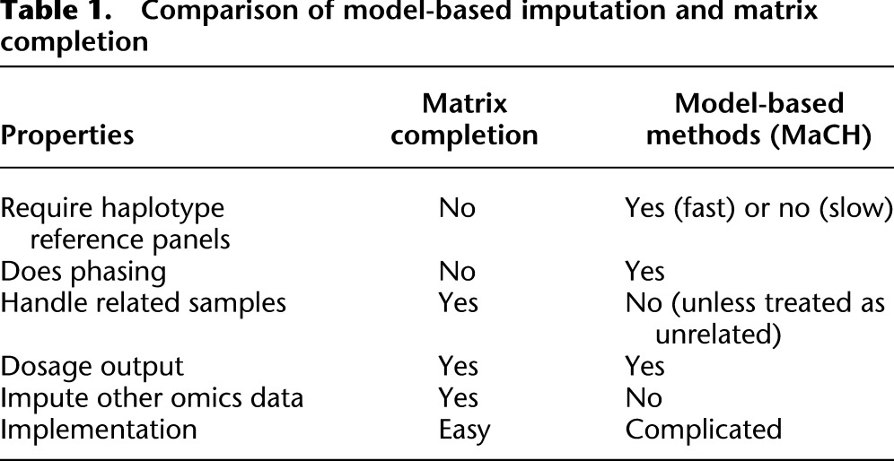
Table 1 compares the virtues of model-based imputation versus matrix completion. As just emphasized, the matrix completion method is off-the-shelf and model agnostic. It does not require reference haplotypes, although it can exploit reference individuals. In principle, it applies to imputation of any genetic data, including human leukocyte antigen (HLA) alleles, CNVs, and insertions and deletions (indels). Its success is predicated on a low rank structure in the data. In the case of genotype data, this assumption is valid over relatively short windows of contiguous SNPs due to linkage disequilibrium. Our judicious implementation of matrix completion in a sliding window yields an effective and fast imputation algorithm. A full description of the algorithm and our program MENDEL-IMPUTE implementing it appear in the Methods section.

Table 1.

Comparison of model-based imputation and matrix completion

Before discussing our results in detail, we briefly review previous applications of machine learning algorithms in genotype imputation. Yu and Schaid (2007) compared several off-the-shelf statistical methods including least angle regression, a machine learning technique that seeks to find the best compromise between model fit and complexity. Matrix completion methods were not among the methods investigated. They concluded that the model-based package fastPHASE by Scheet and Stephens (2006) offered the most accurate and efficient imputations. The gap observed in performance between model-based and machine learning methods may be due to the extreme simplicity of the methods chosen from the latter category. Owing to computational concerns, Yu and Schaid (2007) used only a handful of neighboring SNPs (on the order of tens) to impute any given SNP. Our matrix completion approach allows efficient exploitation of hundreds of neighboring SNPs. We also tune our matrix completion more carefully at the local level because some regions exhibit richer haplotype architectures than other regions. Thus, adaptive tuning is one key to successful application of matrix completion.

Motivated by an earlier Li and Stephens (2003) model, Wen and Stephens (2010) introduced a fast and accurate algorithm based on modeling allele frequencies by a multivariate normal distribution. Their new model relies on a sparse covariance matrix derived by zeroing out weak correlations between SNPs. The general idea is similar to matrix completion. The main difference conceptually and practically is that Wen and Stephens seek parsimony in the SNP domain, whereas we seek parsimony via a low-rank approximation to the observed data. Nonetheless, both methods demonstrate that accurate and fast estimates can be achieved by imposing parsimony at the local level.

Results

We compared MENDEL-IMPUTE to several established software packages in four realistic scenarios. The first two scenarios ignore reference individuals. Scenario 1 relies on a panel of unrelated individuals, while Scenario 2 relies on a moderately sized panel of related individuals. We designed the first two scenarios to assess the raw accuracy of different imputation schemes. The last two scenarios exploit a reference panel from the 1KGP. Scenario 3 considers imputation with a high-density SNP array, while Scenario 4 considers imputation with low-coverage sequencing data. The last two scenarios allow assessment of imputation performance in downstream association analysis. All computations under the four scenarios were done on a multicore computer with four 3.2 GHz Intel Core i7 processors and 12 GB of RAM. The matrix completion algorithm was coded in MATLAB (R2011a). Running times are recorded in seconds using the tic/toc functions of MATLAB.

GWAS without a reference panel

We compared MENDEL-IMPUTE to the popular MaCH software (Li and Abecasis 2006; Li et al. 2009, 2010), considered by many to be the gold standard for imputation accuracy, on the two HapMap panels of 139 Han Chinese (CHB) and 209 Nigerians (YRI). We also included a comparison with fastPHASE (Scheet and Stephens 2006) in Scenario 1, where we imputed genotypes of unrelateds in the absence of a reference panel. In Scenario 1, our goal is to assess imputation accuracy for genotypes missing sporadically. Modern genotyping technology is very accurate, in excess of 98%, and such missing genotypes are relatively rare (Browning and Browning 2007). However, missing values do occur, and it would be a shame to remove individuals or typed markers with a small fraction of missing entries simply as a quality control measure. Dropping such people or SNPs can severely reduce the power of an association study.

We used the unphased genotype data from HapMap. The CHB panel contains only unrelated people, while the YRI panel contains unrelateds plus parent–offspring duos and trios. These two groups also diverge in linkage disequilibrium, with the CHB population exhibiting more and the YRI population exhibiting less. The genotype file merges data from Phase I + II and III HapMap, release 28, build 36 (International HapMap 3 Consortium 2010). Since other popular methods such as BEAGLE and IMPUTE2 have similar accuracy and efficacy trade-offs (Nothnagel et al. 2009), it seemed fair to focus on MaCH as representative for this scenario and the next. The latter two scenarios involving reference panels consider BEAGLE and IMPUTE2 as well.

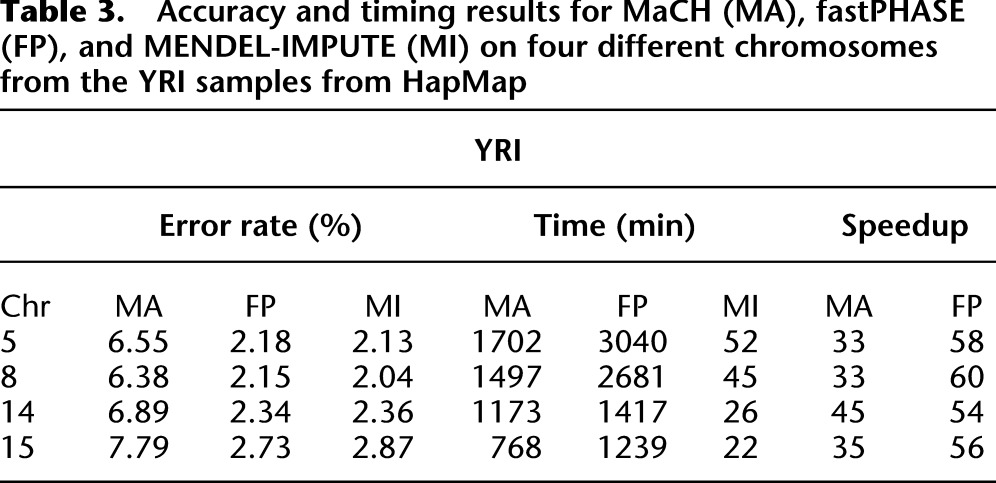
Because subjects were typed on different platforms, the HapMap reference genotype data have almost 50% missing data. To evaluate the performance of the imputation methods on sporadic genotyping errors, however, we randomly masked 1% of the genotyped entries on four randomly selected chromosomes in each group. We then ran the three imputation algorithms on the masked panel and compared imputed entries with masked entries. We defined a genotype error as failing to impute both alleles correctly. Details on experimental setup can be found in the Methods section. Tables 2 and 3 show the accuracy and timing results for MaCH, fastPHASE, and MENDEL-IMPUTE, respectively. MENDEL-IMPUTE uniformly displays lower error rates. What is perhaps even more remarkable is that such accuracy is achieved with a 18-fold to 45-fold reduction in run times compared with MaCH and 16-fold to 60-fold reduction in run times compared with fastPHASE. Note, however, that MaCH can obtain better accuracies by increasing the size of the latent state space and increasing the number of MCMC rounds. Thus, the discrepancy in accuracy is a computational issue reflecting MaCH's trade-offs between accuracy and speed. fastPHASE provided lower error rates, but not necessarily significantly better speeds even in comparison to MaCH. In fact, fastPHASE was much slower on CHB chromosome 5 than MaCH compared with the other CHB chromosomes and also uniformly slower than MaCH on all the YRI chromosomes. Understanding the performance differences requires more detailed understanding of fastPHASE, which is given in Supplemental Note 2. The overall better trade-off between accuracy and speed exhibited by MENDEL-IMPUTE follows from the fact that both fastPHASE and MaCH fix the size of the latent haplotype state space that they use for all points along a chromosome. In contrast to these two methods, MENDEL-IMPUTE dynamically adjusts the model complexity or matrix rank as it moves along the chromosome. BEAGLE also enjoys speedups due to taking a similar strategy of adapting state space complexity as it proceeds along a chromosome.

Table 2.

Accuracy and timing results for MaCH (MA), fastPHASE (FP), and MENDEL-IMPUTE (MI) on four different chromosomes from the CHB samples from HapMap

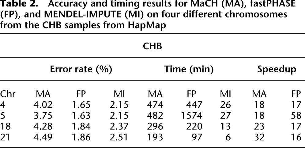
Table 3.

Accuracy and timing results for MaCH (MA), fastPHASE (FP), and MENDEL-IMPUTE (MI) on four different chromosomes from the YRI samples from HapMap

A pedigree sample without a reference panel

We also compared the performance of MaCH and MENDEL-IMPUTE on a sample of moderately sized pedigrees. In the MaCH runs, the subjects are treated as unrelated. The data constitute a subset of 518 individuals spread over 62 pedigrees from a gene mapping study of high plasma angiotensin-1 converting enzyme (Keavney et al. 1998). Genotypes from the original study were ignored. Supplemental Figure 1 displays the distribution of pedigree sizes in our reconfigured sample. Each of the 170 founders in the 62 pedigrees was assigned two unique chromosome 22 haplotypes from the JPT + CHB sample in HapMap 3. Thus, the data reflect realistic genetic assumptions encoded by inferred reference haplotypes rather than observed reference genotypes. We removed SNPs with minor allele frequency below 1% in the 170 founders. This filtering step reduced the original 20,085 typed SNPs to 15,598 SNPs. Finally, we applied the gene dropping option of Mendel 12.0 (Lange et al. 2001) to create synthetic genotypes in the nonfounders consistent with the genotypes of the founders. Gene dropping ignores mutation but includes recombination assuming no interference.

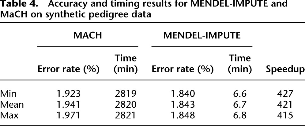
We assessed timing and accuracy for both MaCH and MENDEL-IMPUTE on validation sets formed by holding out a 1% random sample of the data. Details on the parameters used in running MaCH appear in the Methods section. Due to the lengthy run times of MaCH, we report results from just three replicates. For matrix completion, we report results on the same three replicates; timing and error rates were similar on additional replicates. The same set of synthetic genotypes is used in all replicates, and replicates differ only in which entries were masked. Table 4 summarizes our findings. Once again, we see that MENDEL-IMPUTE has a slight edge in imputation accuracy. Both methods may benefit from the perfect typing assumption and the lack of mutation. There is, however, a drastic difference in run times. MENDEL-IMPUTE is more than 400 times faster than MaCH. Compared with Scenario 1, the discrepancy in accuracy is smaller. This scenario is more complicated due to the pedigree structure, but also simpler because we considered a much smaller set of SNPs. In Scenario 1, we considered between 50,000 and 250,000 SNPs. MaCH's improved performance is most likely due to imputing a relatively less diverse set of individuals and also allowing a longer running time for better numerical convergence.

Table 4.

Accuracy and timing results for MENDEL-IMPUTE and MaCH on synthetic pedigree data

There are, of course, ways of imputing missing genotypes in pedigrees that avoid evaluating pedigree likelihoods. The Goradia-Lange algorithm (Lange and Goradia 1987) incorporated in Mendel but not MENDEL-IMPUTE achieves precisely this goal SNP by SNP. The long-range phasing (LRP) algorithm of Kong et al. (2008) exploits whole haplotypes that are identical by descent (IBD). However, pedigree inferences are incapable of resolving all missing genotypes. Methods such as LRP should be viewed as complementary rather than competitive to linkage-disequilibrium methods. In the presence of low genotyping error, the best strategy is apt to be imputation of some genotypes by pedigree methods followed by imputation of remaining genotypes by linkage-disequilibrium methods. In low-coverage sequencing studies, pedigree-based methods may be too error prone to be of much value.

High-coverage genotyping microarray

We next considered the common scenario in GWAS of imputing SNPs from a reference panel typed on a different chip from the study sample. Specifically, we assumed that GWAS data were generated by a high-coverage genotyping microarray, the Illumina's Infinium 2.5M Duo product, which features ∼2.4 million SNPs present in the reference haplotype panel but absent from the chip. The previous two scenarios assessed accuracy at imputing sporadically missing genotype entries, whereas this scenario considers imputing genotypes that are missing because they were not typed.

Both the study panel and the reference haplotypes reflect the 1KGP haplotypes from the March 2012 release of Phase 1. We accordingly downloaded the haplotypes of 1092 1KGP individuals from the IMPUTE2 website (Howie et al. 2009) and split them into a study panel and a reference panel. This division was performed so that the distribution of ethnicities was preserved across both groups. We restricted our attention to 60,000 SNPs from a randomly selected 12-Mb region on chromosome 22 and masked genotypes of all SNPs that were not listed in Illumina's manifest file for the 2.5M Duo. This turned out to be 51,192 SNPs. We then applied MENDEL-IMPUTE, MaCH, BEAGLE, and IMPUTE2 to impute untyped SNPs. We also applied IMPUTE2 after pre-phasing with the rapid haplotype estimator SHAPEIT (Delaneau et al. 2012).

We compared genotype imputation quality in two ways. One reasonable measure is the squared correlation r² between the imputed dosage and the true genotyped dosage at the masked loci. While the unprocessed output of MENDEL-IMPUTE is often sufficient to serve as the imputed dosage for downstream analysis, the immediate estimates are biased toward zero. This is a side effect of the nuclear norm shrinkage applied in our matrix completion algorithm. In cases in which the shrinkage is more pronounced, better performance can be attained by fitting a Gaussian mixture model to the immediate outputs and imputing dosages from the resulting densities. An added benefit of the mixture model is that uncertainty for the imputed values can be assigned. See the Methods section for more details. Here we report results using the mixture model to estimate dosages. The mean r² for MENDEL-IMPUTE was 0.683, while it was 0.751 for MaCH, 0.755 for BEAGLE, 0.801 for IMPUTE2, and 0.779 for SHAPEIT-IMPUTE2. At first blush it appears that MENDEL-IMPUTE is inferior. While imputation inaccuracy does reduce the power of association tests (Pritchard and Przeworski 2001), we provide simulation results that indicate that the loss in power is tolerable given the gains in computational speed. We simulated a quantitative trait arising from a single SNP and checked to see what SNPs came up in an association analysis using the imputed dosages. Details are described in the Methods section.

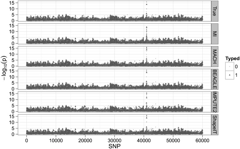
Table 5 shows the resulting comparisons for 10 different trials with different SNPs serving as the trait's major gene. After Bonferroni correction, we checked to see what SNPs were deemed significantly associated with the trait at a significance level of 10⁻³. We refer to the total tally of SNPs deemed significant as “hits.” Table 5 shows that MENDEL-IMPUTE trades a minor dropoff in performance for big reductions in computation time. Thus, despite the excellent agreement in downstream analysis, there is a sizable discrepancy in run times (Table 6). Figure 1 displays the transformed P-values for the 60,000 SNPs when the trait is actually caused by SNP 40,938. For the record, note that MENDEL-IMPUTE may at times produce more hits than the other methods and possibly more false positives. See, for example, the last row in Table 5. There is room for future work in improving how we map MENDEL-IMPUTE's raw output to estimated dosages. We note that SHAPEIT provided noticeable improvement over using IMPUTE2 alone in terms of timing with a small dropoff in accuracy as measured in r². Moreover, although it supports multithreading, we ran SHAPEIT using a single thread for more straightforward comparison with all the other algorithms.

Table 5.

Association analysis results based on Illumina 2.5M microarray data using the 1KGP reference haplotypes

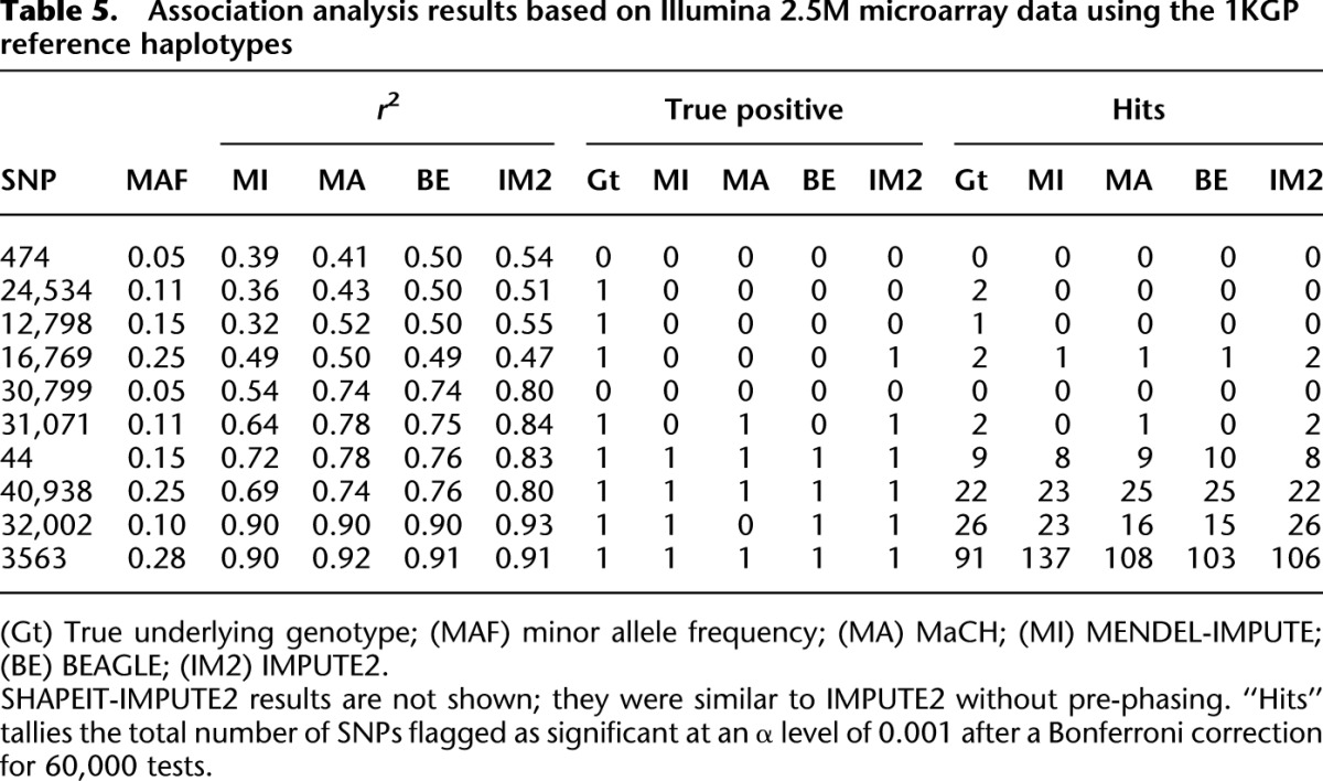
Table 6.

Timing results on high-coverage genotyping microarray data

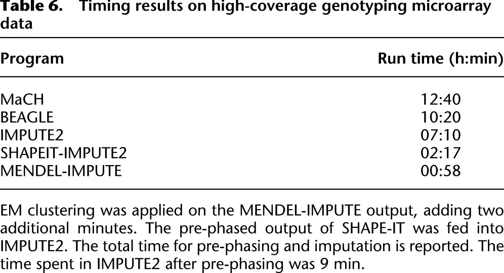
Figure 1.

The negative logarithm of P-values for association when the true signal depends on SNP 40,938. (MI) MENDEL-IMPUTE.

Low-coverage sequencing

We also compared MENDEL-IMPUTE in calling genotypes from low-coverage sequencing data. Pasaniuc et al. (2012) demonstrated that high calling accuracy can be achieved in such data using imputation programs with likelihood scores as inputs. They further demonstrated that the power of imputed genotypes to identify associations in downstream analysis was comparable to that of high-density SNP arrays. Within this framework, we examined how MENDEL-IMPUTE can improve genotype calling of low-coverage sequencing data. In the previous examples, the input to MENDEL-IMPUTE was a matrix with entries drawn from the set {0, 1, 2, missing}. In this scenario, an entry is missing if no reads are recorded for that individual at that locus. Missingness is sporadic as in the first two scenarios but occurs at a much higher rate; in this example, about three-quarters of the entries are missing. The nonmissing input consists of posterior mean dosages with entries in the interval [0, 2]. Dosage levels were computed from paired read counts of the major and minor alleles at each SNP. Details are given in the Methods section.

We used the same study and reference panels as in the previous example, the same 60,000 SNPs on chromosome 22, and the same trait simulations. See the Methods section for details on how the read counts were simulated from the study panel and how posterior mean dosages were computed for input to MENDEL-IMPUTE. As in the previous scenario, accuracy is measured in terms of the r² between the true dosage levels and the estimated dosage levels. In this scenario, since the estimation bias was not as pronounced, we did not re-estimate the dosages via mixture models and instead used the raw MENDEL-IMPUTE output as the estimated dosage. This time the discrepancy in r² was not as drastic as it was 0.854 for MENDEL-IMPUTE, 0.938 for BEAGLE, and 0.80 for IMPUTE2. Tables 7 and 8 report accuracy and timing results for the various programs. MaCH has an extension Thunder for calling genotypes from low-sequencing data, but we did not include it in this example. While it supports input of genotype penetrances, it does not accommodate reference haplotypes. Again, we also assessed the imputation methods on a simulated association testing problem. Compared with BEAGLE and IMPUTE2, MENDEL-IMPUTE suffers marginal decline in association testing and retains a substantial edge in computation time.

Table 7.

Accuracy results on synthetic low-coverage sequencing data

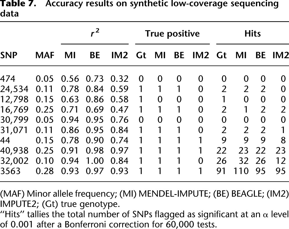
Table 8.

Timing results on synthetic low-coverage sequencing data

Discussion

We have posed genotype imputation as a matrix completion problem and developed an imputation strategy exploiting fast matrix completion algorithms. Numerical experiments demonstrate remarkable accuracy and efficiency for an off-the-shelf method compared with more polished model-based methods. The same strategy readily extends to the imputation of other kinds of omics data such as CNV and RNA-seq. Haplotyping is currently an exception.

Comparing the computational speed of matrix completion to the speed of model-based imputation is complicated by the fundamental differences between the methods. MENDEL-IMPUTE estimates singular vectors that only loosely correspond to a state space of unobserved haplotypes, while model-based methods explicitly invoke haplotypes. The various model-based methods mainly differ in how they simplify their state space. MaCH, IMPUTE2, BEAGLE, and fastPHASE all operate within a hidden Markov model (HMM) framework. The haplotypes that make up the latent state space in MaCH and IMPUTE2 are imperfect mosaics of one another. The complexity of the forward–backward algorithm used to infer latent states scales quadratically in the number of states. IMPUTE2 judiciously chooses a subset of these haplotypes and discards the rest. MaCH chooses a random subset of haplotypes. BEAGLE makes several simplifications to increase scalability: namely, substituting local clusters of haplotypes for latent states, restricting states to emitting only a single type of allele, and restricting the number of possible transitions between states. fastPHASE also simplifies matters by using local haplotype clusters. Thus, the common theme of simplifying the latent state space pervades these HMM programs. MENDEL-IMPUTE adopts an analogous strategy by performing matrix completion over small overlapping windows. The computational complexity of matrix completion scales quadratically in the higher dimension (sample size). This suggests that imputation in large studies be carried out by partitioning the study participants. If good reference haplotypes are provided for each partition, then accuracy may suffer little. In any case, parsimony is achieved by seeking a low-rank approximation over a limited interval of SNPs. For the interested reader, we discuss in Supplemental Note 3 additional illustrative simulation examples that provide some intuition on when MENDEL-IMPUTE is expected to perform both poorly and well. Regardless of the method, however, the moral of the story is that intelligent imposition of parsimony increases speed with little penalty in accuracy.

A possible drawback of matrix completion is that estimated dosages can be biased toward zero. To negate the bias, one can fit mixture models to MENDEL-IMPUTE's immediate output and re-estimate dosages. Doing so also provides estimates for the uncertainty in the estimated dosages. Bias reduction is particularly warranted in imputing untyped SNPs. This is not surprising since the matrix-completion theory gives reconstruction guarantees only when entries are missing at random, which is certainly not the case with untyped SNPs (Candès and Recht 2009). Fortunately, MENDEL-IMPUTE works well after correcting for bias even in a missingness regime not covered by current theory.

Classical quantitative genetics has benefited from rigorous mathematical and statistical models built on Mendelian laws of inheritance and basic principles of population genetics (Elandt-Johnson 1971; Cavalli-Sforza and Bodmer 1999; Lange 2002). These models proved their worth in the era of linkage analysis when data sets were small and matched model assumptions well. As we transition to ever larger and more complex genomics data, it is worth rethinking traditional approaches to statistical analysis. The major stumbling blocks are computational rather than violations of the laws of population genetics. Pedigree data, in particular, will present enormous challenges. Fortunately, the emerging disciplines of data mining and machine learning offer tools for fast prediction, classification, and feature selection in messy high-dimensional data. These tools are desperately needed to fully harvest the fruits of the revolution in experimental data. The balance between modeling and computational feasibility is a delicate one. Fortunately, the information content of modern genomics data is so great that sacrificing some statistical efficiency for finite computation times is not apt to lead geneticists astray.

Methods

Matrix completion

We review the matrix completion problem and describe the algorithm we use to solve it. For the sake of generality, assume that there are p genotyping platforms and that Xⁱ ∈ ℝ^m×n lists the genotyping results for platform i, where m is the number of individuals and n is the number of SNPs. For the sake of simplicity, we assume that all platforms contain the same number of SNPs and that SNPs not typed on a given platform are flagged as missing. Missing entries of Xⁱ arise from several sources. For instance, genotypes can be missing for some entries due to poor genotyping quality. More importantly, a specific platform usually types only a subset of the available SNPs. Thus, many column entries of Xⁱ will be systematically missing. Similarly, many row entries of Xⁱ will be systematically missing because most individuals are typed on only a single platform.

Matrix completion looks for linkage-disequilibrium structure in the matrices Xⁱ over a narrow genomic region. In practice, only a handful of haplotypes occur within a given population over a short region. Accordingly, we expect each Xⁱ to have low rank. One way to impute missing genotypes is to find a low-rank matrix that approximates all Xⁱ well. This suggests the optimization problem

where r denotes an upper bound on the possible rank of Z ∈ ℝ^m×n,

denotes the Frobenius norm of a matrix Y = (y_ij), the set Ω_i indexes the entries that are observed on platform i, and is the projection operator

Besides imputing missing entries in Xⁱ, the optimal Z also effectively resolves inconsistent genotypes among different platforms. Unfortunately, the optimization problem (1) is nonconvex and beset by local minima. Instead, we solve the convex relaxation

where the nuclear norm

(sum of the singular values of Z) serves as a surrogate for the rank function rank(Z), and λ is a positive parameter that tunes the trade-off between model fit and model complexity.

Of the many possible strategies for solving problem (2), we settled on the Nesterov method (Beck and Teboulle 2009) due to its implementation simplicity and good scaling with the dimension of the data. To put its performance in context, the Nesterov method performed slightly better than a close competitor, based on the majorization–minimization (MM) principle (Lange et al. 2000). MM algorithms are widely used in the machine learning, statistics, and signal processing communities because of their numerical robustness, good scaling, and simplicity. Details of our comparison are given in Supplemental Note 1.

Nesterov algorithm

We now describe how we applied Nesterov's algorithm to the matrix completion problem. It simplifies matters to work with a slightly different form of the loss function. Expanding each square in definition (1), it is easy to see that the loss can be rewritten up to an irrelevant constant as

where

and

This formulation has the advantage of permitting incorporation of genotyping quality scores in the model through the weights w_jk. The Nesterov algorithm as summarized in Algorithm 1 consists of two steps per iteration: (a) predicting a search point S^k based on the previous two iterates (line 4); and (b) performing gradient descent from the search point S^k, possibly with a line search (lines 6–11). We first describe Step b. The gradient descent step effectively minimizes the local surrogate function

where c^k is again an irrelevant constant. The first two terms of the surrogate g(Z|S^k, δ) correspond to a linear approximation of f(Z) around the k-th search point S^k. The third term penalizes departures of Z from S^k. This is done to ensure that searching over Z remains within the region for which the linearization of f(Z) is accurate. The nuclear norm penalty is unchanged in moving from f(Z) to g(Z).

Algorithm 1. Nesterov method for minimizing Equation 2.

1 Pre-compute and .

2 Initialize Z⁰, δ > 0, α⁰ = 0, α¹ = 1

3 Repeat

4

5 Repeat

6

7 Compute SVD A_temp = Udiag(a)V^T

8 z ← (a − λδ)₊

9 Z_temp ← Udiag(z)V^T

10 δ ← δ/2

11 until f(Z)_temp ≤ g(Z_temp|S^k, δ)

12 Z^k+1 ← Z_temp

13

14 until objective value converges

The solution to Equation 2 is given by thresholding the singular values of the intermediate matrix S^k − δ∇f(S^k) at λδ. The positive constant δ equals the reciprocal of the Lipschitz constant (f) associated with the gradient of the loss function f(Z). Because this gradient amounts to the Hadamard product

it follows that

with (f) = max_jkw_jk. Consequently, we take δ = (max_jkw_jk)⁻¹. With this specific choice, the linear search described in Algorithm 1 terminates in a single step. Using a larger δ leads to a bigger gradient descent step (line 6), which sometimes must be contracted to send the penalized loss h(Z) = f(Z) + λ‖Z‖ downhill.

We now discuss Step a of Algorithm 1. The search point S^k is found by an extrapolation based on the previous two iterates Z^k and Z^k−1. The Nesterov algorithm accelerates ordinary gradient descent by making this extrapolation. If the global minimum of the penalized loss h(Z) occurs at the point Z*, then the following nonasymptotic bound for the convergence of the objective values

applies (Beck and Teboulle 2009). Without extrapolation, Nesterov's method collapses to a gradient method with the slow nonasymptotic convergence rate of O(k⁻¹) rather than O(k⁻²). Remarkably, the Nesterov method requires essentially the same computational cost per iteration as the unaccelerated gradient method. In practice, convergence is quick for the typical scenarios considered in this study. For example, in the pedigree scenario, the maximum and mean numbers of iterations for a given λ over all imputed windows were 18 and 2.17 iterations.

Matrix completion via MENDEL-IMPUTE

We now describe our strategy for applying matrix completion to genotype imputation. The essential ingredients are imputing genotypes along a sliding window and tuning the penalty constant λ by holding out validation entries of the data matrix.

SNP studies typically consist of 10⁴–10⁶ SNPs and 10²–10⁴ individuals. Since linkage disequilibrium occurs within narrow genomic segments, we apply matrix completion along a sequence of overlapping windows. Each window consists of three subwindows of w SNPs each. Thus, a typical window spans 3w total SNPs. Algorithm 1 is applied to the entire window, but only the middle block of w SNPs is imputed. The window is then shifted over by w SNPs, and the process repeated. The sliding window strategy permits information to propagate from the left and right thirds into the middle third where imputation is performed. The first, second, and last windows are handled somewhat differently. In the first window, the first and middle thirds are simultaneously imputed. The last window encompasses three thirds plus a leftover piece less than w SNPs in length. In the last window, the right third plus the leftover piece are simultaneously imputed.

The tuning constant λ is selected anew for each window by validation in its left and right thirds. In these flanking thirds, we hold out some fraction of entries (typically 10% of the observed entries) and compute the imputation error rate on the masked entries over a grid of λ values. The initial grid always contains k points λ_max, ρλ_max, …, ρ^k−1λ_max determined by a maximum value λ_max and a multiplier ρ ∈ (0, 1). Setting ρ = 1/2 works well in practice. At each of the grid points, we warm start parameter fitting using the values from the previous round of imputation. The grid point with the lowest error rate is then chosen for imputation in the middle third of the window. In practice, a relatively large range of λ yields good accuracy, and a conservative choice of k suffices. Nonetheless, as a safeguard against the possibility that a pre-specified k is too small, we always check whether the error rate bottoms out before we reach the end of the grid ρ^k−1λ_max. If this is not the case, we keep extending the grid downward in a geometric fashion until we see no significant improvement in the error rate. In the results presented in this study, we use k = 11 for our initial grid. Solving Equation 2 for a sequence of λ values suggests using the solution to the problem when λ = ρ^kλ_max as the initial matrix Z⁰ for solving the problem when λ = ρ^k+1λ_max. The benefits of using these warm starts are discussed in more detail in Supplemental Note 1.

Determining the SVD is the most computationally expensive step in the Nesterov algorithm. The Golub-Kahan-Reinsch SVD algorithm implemented in LINPACK/LAPACK and used in MATLAB has computational complexity 4m²n + 8mn² + 9n³ for an m × n matrix (Golub and Van Loan 1996). In our sliding window scheme, we have to choose whether to compute the SVD on a given window or its transpose. The complexity count suggests we should orient matrices so that they are tall and skinny (large m and small n). In our setting, this criterion typically dictates orienting the data matrix so that rows correspond to subjects and columns correspond to SNPs. In this orientation, m is the sample size, and n = 3w is the window width.

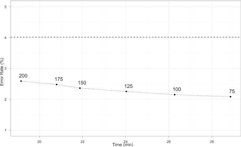
Finally, it remains to determine w. The SVD computation per window takes on the order of 4m²n operations and effectively scales linearly in w rather than cubically. At the same time, however, it takes fewer windows to cover the entire chromosome when windows are wider. Also, imputation accuracy depends on w. To assess the complex trade-offs in accuracy versus run time, we performed a battery of comparisons on HapMap 3 panels over six values of w ranging from 75 to 200. Figure 2 shows results for the Nesterov matrix completion algorithm for the chromosome 4 CHB data from HapMap 3. Error rates are estimated from a 1% hold-out set. Details on the data appear in the next section, where we discuss comparisons with MaCH. Results for additional chromosomes and other ethnic groups are summarized in Supplemental Figures 2 and 3. The bottom line is that model-free imputation is remarkably accurate over a very wide range in w. Both run time and accuracy slightly decrease as w increases over the range investigated. For comparison, the dashed line shows the error rate for MaCH on the same data.

Figure 2.

Accuracy versus time trade-off for the Nesterov algorithm on chromosome 4 from the Chinese Han group in HapMap 3. The numbers indicate the subwindow size w. (Dashed line) Error rate for MaCH on the same data set.

Posterior probabilities, dosage estimates, and estimation error

In this section, we describe how to assign posterior probabilities, and consequently dosage estimates, to the raw output from MENDEL-IMPUTE. Suppose we measure a random scalar attribute x_i for each of n objects 1, …, n. Each object must be assigned to one of k latent clusters. Let C_ij denote the event that object i belongs to cluster j, h_j(x|θ) the density of the attribute conditional on the object belonging to cluster j, and π_j the probability that any object belongs to cluster j. Further suppose that (π₁, …, π_k) has Dirichlet(a₁, …, a_k) prior. If z_ij is the indicator function of the event C_ij, then joint likelihood of the data and parameters is proportional to

If we further assume that the conditional densities h_j(x|θ) are normally distributed with means μ_j and common variance σ², then the EM algorithm for obtaining maximum a posteriori estimates of the μ_j, π_j, and σ² proceeds by cyclically applying the following four updates:

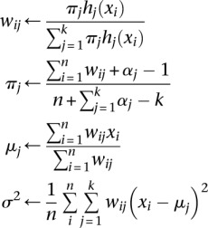until convergence. See the discussion on EM clustering in Lange (2012) for a derivation of these updates. Additional details such as how to initialize the EM algorithm and how to choose the parameters α_j can be found in Supplemental Note 4. With these posterior probabilities in hand, one can then impute the reference allele dosages at a given SNP by computing posterior mean counts of the reference allele. A genotype can be assigned to the cluster with the greatest posterior probability. Moreover, the posterior probabilities calibrate the uncertainty in the imputed dosages. An example, comparing the raw MENDEL-IMPUTE output and the final imputed dosage for a SNP, appears in Supplemental Figure 4.

Experimental details

All reported results for matrix completion rely on a fixed window size of w = 100 and k_min = 11 regularization parameter grid points. As just mentioned, the performance of the matrix completion algorithm is very stable with respect to these settings. Higher efficiency with little compromise in accuracy can be achieved using a larger window size.

HapMap 3

Note that the SNPs reported in HapMap have already undergone quality control screening, including removal of SNPs with low call rates and extreme deviations from Hardy-Weinberg equilibrium. Aside from removing relatively rare indel SNPs, we did no further pre-processing before applying the two imputation methods. Details on quality control screening in the HapMap panels appears in the supplementary section of International HapMap 3 Consortium (2010).

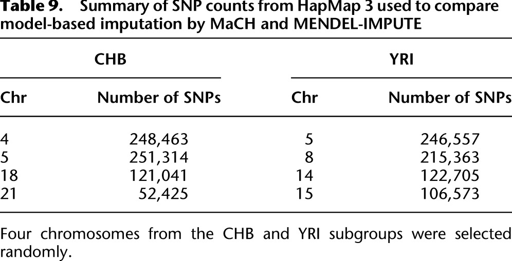
Table 9 summarizes the number of SNPs in each of the four randomly selected chromosomes in our comparisons. For each SNP, a reference allele is given in the HapMap panel. These do not necessarily correspond to the minor or major allele. For our matrix completion algorithm, we used a dosage model based on the reference allele to code entries in the data matrix, namely, 0 for homozygosity in the reference allele, 1 for heterozygosity, and 2 for homozygosity in the nonreference allele. While assigning the minor allele to be the reference allele is a natural choice, doing so is not necessary. Since the matrix completion algorithm returns real values, we mapped these back to elements in the set {0, 1, 2} by simply rounding to the closest integer in the set. Applying the EM-clustering algorithm gave similar results. We ran MaCH using the option flags -geno, -mle, and -compact and omitting a reference panel. We ran fastPHASE 1.4.0 using the option flags -H-4 -T10 -C25 to turn off haplotype estimation, limit the number of random starts and EM iterations, and thus ultimately save on computation time.

Table 9.

Summary of SNP counts from HapMap 3 used to compare model-based imputation by MaCH and MENDEL-IMPUTE

Synthetic pedigree

To assess the performance of MaCH in the synthetic pedigree example, we applied the two-stage procedure recommended for large data sets. Thus, we used a random subsample of 200 individuals to estimate the crossover and error rates. We ran MaCH again over the entire set of 518 individuals, passing in the two parameters estimated from the first stage. In both stages, we used 50 rounds of Monte Carlo sampling and 200 hidden haplotype states.

High-coverage genotyping microarray

The simulated quantitative trait y_i for individual i depends on the dosage x_i of a single SNP according to the model:

where μ = 160, β = 3, σ = 5, and the ɛ_i are i.i.d. standard normal. Ten different SNPs are used to generate the trait signals for 10 different trials. SNPs vary in reference allele frequency and squared correlation r² between their imputed dosages and their true dosages. MaCH, BEAGLE, IMPUTE2, and SHAPEIT-IMPUTE2 were applied using their default values.

Low-coverage sequencing

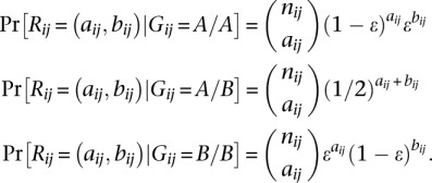
We calculate the likelihoods of genotype dosages using a standard binomial model (Sampson et al. 2011; Pasaniuc et al. 2012). To explain the model, let G_ij denote the latent genotype at SNP i for individual j, A and B the major and minor alleles at the SNP, and R_ij = (a_ij, b_ij) the read count pair for i over A and B, respectively. If there is a fixed per-base per-read error rate of ɛ, and n_ij = a_ij + b_ij, then the conditional likelihoods of R_ij amount to

Sampson et al. (2011) observed that the distribution of coverage was observed to be well described empirically by a negative binomial distribution. They therefore advocated modeling the number of reads N_ij ∼ Poisson(μ × γ_i), where μ denotes the average coverage and γ_i ∼ Γ(α, β) with shape parameter α and scale parameter β = 1/α. In the simulation studies, we sample the number of reads at locus i as Poisson with γ_i ∼ Γ(3.8, 0.8) and μ fixed at 1. This procedure gave coverage statistics in line with those observed in Phase 1 1KGP.

To convert the sequence data into a form suitable for MENDEL-IMPUTE, we constructed a matrix of posterior mean dosages based on the Hardy-Weinberg priors:

where p_A and p_B are the empirical allele frequencies from the reference panel. The Bayes rule implies that the posterior probabilities Pr(G_ij|R_ij, n_ij) can be recovered via

with normalizing constant

Finally, if A is the reference allele, then the posterior mean dosage is expressed as

For low coverage sequencing data, the total reads n_ij at SNP i for person j served as a weight w_ij in the matrix completion criterion:

Reference haplotypes were incorporated in a matrix H with entries h_ij ∈ {0, 1}, and the data matrix X was expanded to . MENDEL-IMPUTE was then applied to the data matrix with weight matrix , where .

For each SNP, a gamma distributed random variable γ was drawn. To determine the number of reads, a Poisson deviate with intensity γ was then drawn. Each haplotype was sampled with equal probability, and errors were introduced in reading with probability ɛ = 0.01. Read data were converted to posterior mean dosages to obtain the matrix X. We then applied MENDEL-IMPUTE to the composite matrix using the weights just described. Finally, we projected the estimated entries z_ij onto the interval [0, 2].

Software availability

Our MATLAB code implementing MENDEL-IMPUTE is freely available at http://www.genetics.ucla.edu/software/. MENDEL-IMPUTE will also be available as an option in the comprehensive genetic analysis software Mendel distributed on the same website.

References

- The 1000 Genomes Project Consortium 2010. A map of human genome variation from population-scale sequencing. Nature 467: 1061–1073 [DOI] [PMC free article] [PubMed] [Google Scholar]
- Ayers KL, Lange K 2008. Penalized estimation of haplotype frequencies. Bioinformatics 24: 1596–1602 [DOI] [PubMed] [Google Scholar]
- Beck A, Teboulle M 2009. A fast iterative shrinkage-thresholding algorithm for linear inverse problems. SIAM J Imaging Sci 2: 183–202 [Google Scholar]
- Browning SR, Browning BL 2007. Rapid and accurate haplotype phasing and missing-data inference for whole-genome association studies by use of localized haplotype clustering. Am J Hum Genet 81: 1084–1097 [DOI] [PMC free article] [PubMed] [Google Scholar]
- Browning BL, Browning SR 2009. A unified approach to genotype imputation and haplotype-phase inference for large data sets of trios and unrelated individuals. Am J Hum Genet 84: 210–223 [DOI] [PMC free article] [PubMed] [Google Scholar]
- Cai J-F, Candès EJ, Shen Z 2010. A singular value thresholding algorithm for matrix completion. SIAM J Optim 20: 1956–1982 [Google Scholar]
- Candès EJ, Recht B 2009. Exact matrix completion via convex optimization. Found Comput Math 9: 717–772 [Google Scholar]
- Cavalli-Sforza L, Bodmer W 1999. The genetics of human populations. Dover Publications, Mineola, NY [Google Scholar]
- Delaneau O, Marchini J, Zagury J-F 2012. A linear complexity phasing method for thousands of genomes. Nat Methods 9: 179–181 [DOI] [PubMed] [Google Scholar]
- Elandt-Johnson RC. 1971. Probability models and statistical methods in genetics. Wiley, New York. [Google Scholar]
- Golub GH, Van Loan CF 1996. Matrix computations, 3rd ed. Johns Hopkins Studies in the Mathematical Sciences. Johns Hopkins University Press, Baltimore [Google Scholar]
- Howie BN, Donnelly P, Marchini J 2009. A flexible and accurate genotype imputation method for the next generation of genome-wide association studies. PLoS Genet 5: e1000529. [DOI] [PMC free article] [PubMed] [Google Scholar]
- The International HapMap 3 Consortium 2010. Integrating common and rare genetic variation in diverse human populations. Nature 467: 52–58 [DOI] [PMC free article] [PubMed] [Google Scholar]
- Keavney B, McKenzie CA, Connell JMC, Julier C, Ratcliffe PJ, Sobel E, Lathrop M, Farrall M 1998. Measured haplotype analysis of the angiotensin-I converting enzyme gene. Hum Mol Genet 7: 1745–1751 [DOI] [PubMed] [Google Scholar]
- Kong A, Masson G, Frigge ML, Gylfason A, Zusmanovich P, Thorleifsson G, Olason PI, Ingason A, Steinberg S, Rafnar T, et al. 2008. Detection of sharing by descent, long-range phasing and haplotype imputation. Nat Genet 40: 1068–1075 [DOI] [PMC free article] [PubMed] [Google Scholar]
- Koren Y, Bell R, Volinsky C 2009. Matrix factorization techniques for recommender systems. Computer 42: 30–37 [Google Scholar]
- Lange K. 2002. Mathematical and statistical methods for genetic analysis, 2nd ed. Statistics for Biology and Health. Springer-Verlag, New York. [Google Scholar]
- Lange K. 2012. Optimization, 2nd ed. Springer Texts in Statistics. Springer-Verlag, New York. [Google Scholar]
- Lange K, Goradia TM 1987. An algorithm for automatic genotype elimination. Am J Hum Genet 40: 250–256 [PMC free article] [PubMed] [Google Scholar]
- Lange K, Hunter DR, Yang I 2000. Optimization transfer using surrogate objective functions. J Comput Graph Statist 9: 1–20 [Google Scholar]
- Lange K, Cantor R, Horvath S, Perola M, Sabatti C, Sinsheimer J, Sobel E 2001. Mendel version 4.0: A complete package for the exact genetic analysis of discrete traits in pedigree and population data sets. Am J Hum Genet 69: 50411462172 [Google Scholar]
- Li Y, Abecasis G 2006. MaCH 1.0: Rapid haplotype reconstruction and missing genotype inference. Am J Hum Genet S79: 2290 [Google Scholar]
- Li N, Stephens M 2003. Modeling linkage disequilibrium and identifying recombination hotspots using single-nucleotide polymorphism data. Genetics 165: 2213–2233 [DOI] [PMC free article] [PubMed] [Google Scholar]
- Li Y, Willer C, Sanna S, Abecasis G 2009. Genotype imputation. Annu Rev Genomics Hum Genet 10: 387–406 [DOI] [PMC free article] [PubMed] [Google Scholar]
- Li Y, Willer CJ, Ding J, Scheet P, Abecasis GR 2010. Mach: Using sequence and genotype data to estimate haplotypes and unobserved genotypes. Genet Epidemiol 34: 816–834 [DOI] [PMC free article] [PubMed] [Google Scholar]
- Marchini J, Howie B 2010. Genotype imputation for genome-wide association studies. Nat Rev Genet 11: 499–511 [DOI] [PubMed] [Google Scholar]
- Marchini J, Howie B, Myers S, McVean G, Donnelly P 2007. A new multipoint method for genome-wide association studies by imputation of genotypes. Nat Genet 39: 906–913 [DOI] [PubMed] [Google Scholar]
- Mazumder R, Hastie T, Tibshirani R 2010. Spectral regularization algorithms for learning large incomplete matrices. J Mach Learn Res 11: 2287–2322 [PMC free article] [PubMed] [Google Scholar]
- Nothnagel M, Ellinghaus D, Schreiber S, Krawczak M, Franke A 2009. A comprehensive evaluation of SNP genotype imputation. Hum Genet 125: 163–171 [DOI] [PubMed] [Google Scholar]
- Pasaniuc B, Rohland N, McLaren PJ, Garimella K, Zaitlen N, Li H, Gupta N, Neale BM, Daly MJ, Sklar P, et al. 2012. Extremely low-coverage sequencing and imputation increases power for genome-wide association studies. Nat Genet 44: 631–635 [DOI] [PMC free article] [PubMed] [Google Scholar]
- Pritchard JK, Przeworski M 2001. Linkage disequilibrium in humans: Models and data. Am J Hum Genet 69: 1–14 [DOI] [PMC free article] [PubMed] [Google Scholar]
- Sampson J, Jacobs K, Yeager M, Chanock S, Chatterjee N 2011. Efficient study design for next generation sequencing. Genet Epidemiol 35: 269–277 [DOI] [PMC free article] [PubMed] [Google Scholar]
- Scheet P, Stephens M 2006. A fast and flexible statistical model for large-scale population genotype data: Applications to inferring missing genotypes and haplotypic phase. Am J Hum Genet 78: 629–644 [DOI] [PMC free article] [PubMed] [Google Scholar]
- Wen X, Stephens M 2010. Using linear predictors to impute allele frequencies from summary or pooled genotype data. Ann Appl Stat 4: 1158–1182 [DOI] [PMC free article] [PubMed] [Google Scholar]
- Yu Z, Schaid D 2007. Methods to impute missing genotypes for population data. Hum Genet 122: 495–504 [DOI] [PubMed] [Google Scholar]