iReckon: Simultaneous isoform discovery and abundance estimation from RNA-seq data

Abstract

High-throughput RNA sequencing (RNA-seq) promises to revolutionize our understanding of genes and their role in human disease by characterizing the RNA content of tissues and cells. The realization of this promise, however, is conditional on the development of effective computational methods for the identification and quantification of transcripts from incomplete and noisy data. In this article, we introduce iReckon, a method for simultaneous determination of the isoforms and estimation of their abundances. Our probabilistic approach incorporates multiple biological and technical phenomena, including novel isoforms, intron retention, unspliced pre-mRNA, PCR amplification biases, and multimapped reads. iReckon utilizes regularized expectation-maximization to accurately estimate the abundances of known and novel isoforms. Our results on simulated and real data demonstrate a superior ability to discover novel isoforms with a significantly reduced number of false-positive predictions, and our abundance accuracy prediction outmatches that of other state-of-the-art tools. Furthermore, we have applied iReckon to two cancer transcriptome data sets, a triple-negative breast cancer patient sample and the MCF7 breast cancer cell line, and show that iReckon is able to reconstruct the complex splicing changes that were not previously identified. QT-PCR validations of the isoforms detected in the MCF7 cell line confirmed all of iReckon's predictions and also showed strong agreement (r² = 0.94) with the predicted abundances.

Accurate methods for RNA-seq data analysis are proving essential for characterization of gene regulation and function, as well as understanding development and disease (Lopezbigas et al. 2005; Kim et al. 2008; Wang et al. 2009). The plethora of alternative isoforms present for many human genes significantly extend the repertoire of proteins, and this source of variation has been linked to human disorders, including cancer (Shah et al. 2012). The identification of the full set of transcripts present in a tissue, especially those present at low abundance, remains challenging. Transcriptome analysis from RNA-seq data typically involves solving two subproblems:

1. Identification of the set of isoforms present in the data, and

2. Estimation of the abundance of these isoforms.

The first problem is challenging due to the incomplete nature of RNA-seq data, with only two (paired) short reads generated from each fragment of RNA. The second problem is complicated by the plethora of sequencing biases present within a typical RNA-seq data set, including base content and location within the isoform, as well as PCR amplification bias, which results in multiple reads generated from a single original fragment.

Some of the earlier methods for RNA-seq analysis addressed either the identification or the quantification problem. For identification, methods such as TopHat (Trapnell et al. 2009) and MapSplice (Wang et al. 2010) align raw sequencing reads to the genome in ways that allow for the discovery of novel isoforms and identification of alternative and aberrant splicing events. For quantification, early methods simply counted the number of fragments mapping to each input isoform to compute its abundance. However, recent methods have significantly improved on this and have allowed for the correction of many systematic biases. One such problem is the interdependence of the assignment of reads to isoforms and the expression of the genes. While the assignment of a read to an isoform clearly changes the abundance prediction of this isoform, the converse is also true: The likelihood that a read was drawn from a particular isoform is proportional to its expression. This problem can be elegantly solved by using the expectation-maximization (EM) algorithm as previously shown in Nicolae et al. (2011) and Li et al. (2010). Here, reads are assigned to isoforms based on an initial estimate of each isoform's abundance, and the estimates are recomputed based on the reads. This process is iterated until it converges. One drawback of the EM-based approaches is overfitting: All isoforms provided to the program are assigned a (possibly very low) abundance, even if they are not expressed.

To prevent overfitting, some approaches, like Cufflinks (Trapnell et al. 2010), rely on parsimony and identify the minimum set of isoforms necessary to explain the observed read data and then reconstruct their abundance. Alternatively, RQuant (Bohnert and Rätsch 2010) uses regularized quadratic optimization to correct for various sequencing biases in the more global coverage signal. One recent approach (Feng et al. 2011) identified the importance of solving the two problems simultaneously. Indeed, accurate estimation of isoform abundance is extremely difficult if not all isoforms are known, as the read pairs generated from unidentified isoforms can affect the quantity estimation of known ones. Abundance estimation can be used to inform isoform reconstruction: Incoherent abundances likely indicate that some isoforms were missed by the reconstruction stage. In this context, IsoInfer/IsoLasso (W Li et al. 2011) was the first tool to simultaneously solve both identification and quantification problems by computing a large set of possible isoforms and then using LASSO (Tibshirani 1996) to select a subset of these that best explain the observed abundances.

In this article, we present iReckon, an algorithm for simultaneous isoform reconstruction and abundance estimation. To our knowledge, our method is the first to combine maximum likelihood–based abundance estimation with analysis of a large number of feasible isoforms in order to allow for novel isoform detection. While the large number of parameters would typically lead to overfitting, our method is based on the regularized EM algorithm (Li et al. 2005) with a novel, nonlinear regularization penalty to eliminate isoforms with marginal support. This allows for the quantification and discovery of novel isoforms even with very low expression. To speed up this algorithm, we introduce several computational heuristics. Additionally, our method is the first to directly model several biological and technical phenomena, including the presence of unspliced pre-mRNA, intron retention, and PCR amplification bias. Supplemental Figure S1 summarizes the key features of iReckon and compares these to other popular tools.

We have evaluated the performance of iReckon using both simulated data, with a known ground truth, and using several real Illumina RNA-seq data sets, where we explore the method's ability to recapitulate previously known human transcripts. Additionally, we apply our method to two cancer transcriptomes and demonstrate its ability to discover complex splicing patterns (confirmed by QT-PCR) that are missed by other methods.

Results

In this section, we first present a brief outline of the iReckon algorithm, with additional details presented in the Methods section. We then evaluate the performance of iReckon on both simulated and real RNA-seq data and compare it to three popular existing algorithms, Cufflinks (Trapnell et al. 2010), SLIDE (J Li et al. 2011), and IsoLasso (W Li et al. 2011). Finally, we use iReckon to explore the transcriptomes of two breast cancer data sets—a patient sample recently sequenced at the BC Genome Sciences Center (Shah et al. 2012) and the MCF7 cell line (accession no. SRX040504) (Sun et al. 2011).

iReckon algorithm overview

The iReckon workflow consists of three stages: (1) the identification of all possible isoforms, (2) realignment of reads to these isoforms, and (3) the reconstruction of abundances of every putative isoform. iReckon then reports isoforms with positive abundances. These three steps are overviewed within the next three subsections. Subsequently, we describe a visualization tool for transcriptomic data that we have developed for use with iReckon or any similar method. The details of the methods and models are described in the Methods section, as are the running time and memory requirements of iReckon.

Reconstruction of possible isoforms

The first step of iReckon is the identification of isoforms possibly present within the sequenced sample. While iReckon will accept a set of annotations, we also align all of the reads to the genome using an algorithm that allows for split-mapping. We used TopHat (Trapnell et al. 2009) for this task, though another tool could be used instead. The alignments and the known isoforms are used to generate the set of all observed and known splice junctions, which in turn are used to construct splicing graphs (Heber et al. 2002) that represent the isoforms possibly present within the sample. Note that the information about splice junctions can help us determine most alternative splicing events (exon skipping, alternative donor/acceptor sites, etc.), except intron retention, which is discussed in Isoforms Reconstruction Model Extensions in the Methods section. For each graph, we then enumerate all paths from each of the possible transcription start sites to the end sites. Each such path corresponds to an isoform, and we further add isoforms corresponding to pre-mRNA and any putative intron retention events detected by our intron retention statistical model (see Isoforms Reconstruction Model Extensions). The total number of paths through the splicing graph can potentially be extremely large. In such rare cases, we prioritize the splice sites based on the number of reads split-mapped across each site and select up to 100,000 paths through the graph with the highest support.

Realigning the reads

For each putative isoform, we extract its corresponding DNA sequence and realign the paired reads to the set of all possible isoforms. This step allows for the direct (without splitting) alignment of each read and allows us to use more sensitive alignment tools, resulting in having more reads correctly aligned. This step also corrects for coverage biases near exon junctions due to alignment difficulty. Note that each read pair can align not just to multiple isoforms within a gene but also to multiple genes. Each pair is assigned an initial affinity for each isoform to which it was aligned. This affinity is based on the alignment score and the inferred insert length (for details, see Alignments and Resulting Optimizations).

Isoform selection and abundances estimation

Finally, we simultaneously determine the set of isoforms present in the data and estimate their abundances by using a regularized EM algorithm on the set of possible isoforms. The standard EM algorithm iteratively estimates the abundance of each isoform based on the read pairs currently assigned to it, and then reallocates the pairs to isoforms based on both alignment scores and the isoforms' estimated expression levels. Because the allocation of reads to isoforms depends on their expression, the process needs to be iterated multiple times until it converges. The standard EM algorithm would assign most isoforms a positive (though possibly very low) abundance. However, this is likely to lead to inaccuracies, especially in our case, as iReckon considers the space of all possible isoforms, with most not expected to be present in the sample. To balance between maximizing the likelihood of the data and the simplicity (number of isoforms) in the model, we introduce a regularization penalty. While the ideal objective would be to directly penalize the number of isoforms (or parameters; L0-norm) (McLachlan and Peel 2000), optimizing such an objective is computationally intractable, so the sum of the parameters (L1-norm, or LASSO) is commonly used as a regularizer. However, as we explain in the Regularized EM Algorithm section in the Methods, this is not appropriate for abundances, so we introduce a novel regularization penalty based on a concave function. We also extend the standard EM algorithm to properly handle PCR duplicates (see Accounting for PCR Duplicates). The isoforms with positive estimated abundances at the convergence of the regularized EM are considered present in the sample and are reported by the algorithm.

Visualization

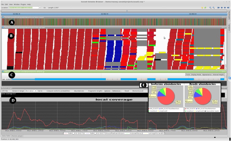
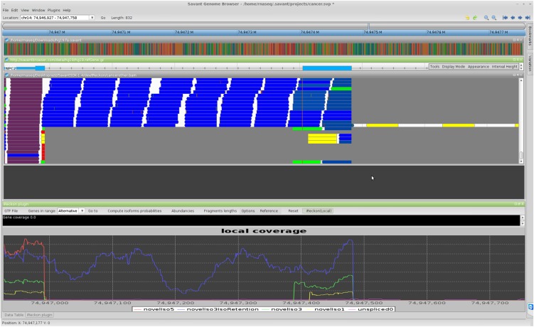
We have found visualization of the RNA-seq data essential during the development of our method and validation of novel isoforms, as well as an effective way to evaluate the tool's performance. To enable effective visualization we have developed an RNA-seq analysis plug-in within the Savant Genome Browser (Fiume et al. 2010, 2012). The RNA-seq Analyzer plug-in displays the reads aligned to the genome, computes for each read the probabilities of isoform of origin (these are visualized by coloring the reads), and visualizes the coverage signal for each isoform. A local version of iReckon is also implemented within the plugin and allows isoforms reconstruction and abundances estimation from the reads' alignments to a single selected gene. Figure 1 displays the interface of this plugin, which can be downloaded from http://savantbrowser.com.

Figure 1.

Screen shot of Savant transcriptome analysis plug-in (RNA-seq Analyzer). (A) Track for the reference genome. (B) Track visualizing aligned reads, with the color representing their isoform of origin probabilities. (C) Known isoform annotation from UCSC. (D) The estimated coverage signal for the various isoforms detected by iReckon. If two RNA-seq data sets are loaded, one can also view differences between abundances of each isoform in the two data sets. Note that the blue isoform has an intron retention event (middle). Because this isoform corresponds to a non-negligible fraction of the overall gene expression level, the failure to identify this event may lead to inaccuracy in quantifying the other isoforms. Additionally, iReckon identifies and quantifies the canonical isoform (in red), the pre-mRNA (in yellow,) and an additional isoform with an alternative donor site (in green). (E) An alternative view of the relative isoform abundances and proportions of reads assigned to each isoform are provided via pie charts. In B and E, black reads are those that could not be assigned to any detected isoforms.

Performance comparison on simulated data

Since there is no ground truth for any real transcriptomic data set, simulating realistic RNA-seq data is a standard method for comparing RNA-seq tools. We generated an RNA-seq data set based on known human isoforms, while also introducing various alternative splicing events (see RNA-seq Data Simulation) and utilized it to quantify the performance of iReckon and three other programs that perform both isoform abundance estimation and novel transcript discovery: Cufflinks, IsoLasso, and SLIDE. We aligned the simulated data with TopHat and gave the four methods the library of all known human isoforms to use as a guide. To compare the methods, we evaluate their recall (TP/(TP + FN); fraction of true isoforms, known or novel, identified by the method), precision (TP/(TP + FP); fraction of reported isoforms, known or novel, that are correct), as well as abundance estimation accuracy. To compute these measures, we consider transcripts with positive abundance reported by each method. We separate isoforms into high, medium, and low abundance, based on the simulated isoform abundance as a fraction of the total simulated data (>10⁻³, 10⁻³ > x > 5 × 10⁻⁵, and <5 × 10⁻⁵, respectively). These three classes make up 5%, 69%, and 26% of all isoforms. In these results, we did not consider isoforms corresponding to unspliced pre-mRNA as this is only discovered and estimated by iReckon.

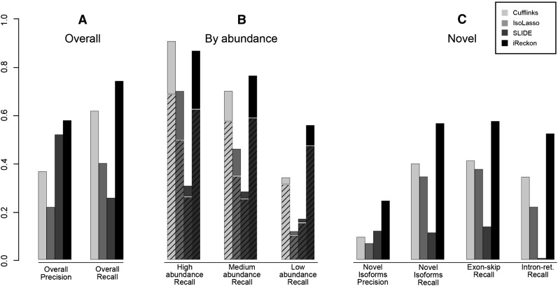
Figure 2A shows a comparison of the four methods at isoform discovery. iReckon achieves the highest recall and precision. Figure 2B demonstrates the method's ability to identify isoforms depending on their level of expression. While all methods perform better at high-abundance isoforms than low-abundance ones, iReckon's performance degrades the least of the four methods. Notably, iReckon's recall for novel low-abundance isoforms is three times that of the other methods (solid section of the bar). This is likely due to the fact that iReckon uses efficient regularization and that isoforms with unambiguous evidence in the data are still reported, even at low abundance. In contrast, all other methods filter out isoforms using abundance thresholds. To compare the power of the different methods at discovering novel isoforms, in Figure 2C, the recall and precision are computed by only considering novel isoforms (novel simulated and novel found). iReckon's precision is ∼200% higher and its recall is 50% higher than other methods of identifying novel isoforms from RNA-seq data.

Figure 2.

Ability of the different methods to discover simulated isoforms. Simulation contains 2533 known isoforms (provided to the methods) and 1006 novel isoforms (811 exon skips, 195 intron retentions). (A) Overall precision and recall for discovering simulated isoforms (known + novel). (B) Recall for isoforms based on level of expression. (Hashed bars) Proportion of known isoforms; (solid bars) novel isoforms. While Cufflinks slightly outperforms iReckon on discovery of known isoforms with high abundance, the results on low-abundance isoforms are reversed, and iReckon outperforms the other methods at identification of all novel isoforms (size of solid sections of bars). (C) Precision and recall for discovery of novel isoforms, as well as recall specific to different types of alternative splicing simulated.

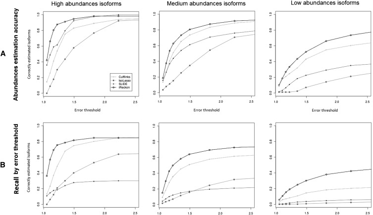
To evaluate the abundance estimation accuracy of each method, we compared the predicted isoform abundance of each correctly identified isoform to its true (simulated) abundance. We computed, for each isoform, the abundance error as the ratio between the true and predicted abundance estimates, larger over smaller. Figure 3A demonstrates the abundance estimation accuracy for each of the four methods depending on the error threshold. Here iReckon clearly outperforms Cufflinks, SLIDE, and IsoLasso across all three abundance classes and for all error thresholds. The full data are presented as scatterplots in Supplemental Figure S11. In terms of median per-isoform abundance deviation (deviation = error − 100%), iReckon outperformed the other methods on high-, medium-, and low-abundance classes with 8%, 14%, and 48% median deviation, respectively. Cufflinks, the second-best method overall, had 18%, 20%, and 70% median deviation on the same classes, and SLIDE has a median deviation of 11% on the fewer high-abundance isoforms it discovers. iReckon thus demonstrated a significantly better global accuracy than Cufflinks (P-value of 8.06 × 10⁻¹⁸, Wilcoxon signed rank test). Box plots associated with these results are presented in Supplemental Figure S12.

Figure 3.

Abundance estimation accuracy and isoform detection recall depending on the acceptable error threshold. (A) Abundance estimation accuracy for correctly predicted isoforms. The three plots show the fraction of correctly estimated isoforms depending on the acceptable error rate (isoforms with error above threshold have incorrect abundances) for high-, medium-, and low-abundance isoforms. While performance is best for high-abundance isoforms for all methods, iReckon outperforms other methods for all three categories and regardless of the error threshold. (B) Isoform detection recall depending on the acceptable error rate (isoforms with error above the threshold are considered “not predicted”). iReckon outperforms the other methods, especially for low-abundance isoforms.

Figure 3B shows each method's recall based on the abundance estimation error. In this case, an isoform is not considered predicted correctly if its abundance is misestimated beyond the given error threshold. Here iReckon also greatly outperforms the other methods, due to both its better overall recall and its higher abundance accuracy.

Performance comparison with Illumina BodyMap2 RNA-seq data

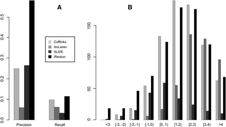
To further test the ability of iReckon to identify novel isoforms in real RNA-seq data, we used an Illumina BodyMap2 muscle transcriptome data set (NCBI SRA accession ERR030876), which consisted of ∼82 × 10⁶ pairs of 50 bp-long reads. Starting with the 36,796 RefSeq human transcripts we left out 7842 random isoforms to be used for testing, while the remaining 28,242 isoforms were provided to the RNA-seq analysis methods. While there are novel isoforms that are present in any tissue, overall we expect a large fraction of true transcripts within the RNA pool to be known. To evaluate each of the methods, we computed precision as the ratio of the previously known isoforms identified by each tool to all of its predictions, and recall as the fraction of the left-out isoforms that were predicted as present by each method. The results are summarized in Figure 4A.

Figure 4.

(A) The precision of the four methods at identifying known genes and their recall for discovering novel (hidden) isoforms from Illumina RNA-seq data. (B) Histogram of the abundances of hidden isoforms (re-)discovered by each method. The x-axis units are log (RPKM).

Overall, Cufflinks and SLIDE respectively identified 69,186 and 19,602 isoforms from the RNA-seq data, of which 17,072 and 5137 were known human transcripts (precision = 0.25 and 0.26). IsoLasso identified 81,086 transcripts, of which only 4514 were known, corresponding to a precision of 0.06. iReckon, demonstrated the highest precision (0.58), identifying 26,848 isoforms, of which 15,623 were known. The 8554 isoforms that were not provided to the tools were then used to evaluate the recall of various algorithms at predicting novel isoforms. Note that we do not expect all of these 7842 to be expressed within this sample; however, an overall higher recall (at equal precision) is indicative of better performance. iReckon identified 827 of these isoforms (recall = 0.11) as present in the sample, followed by Cufflinks with 771 (recall = 0.10), IsoLasso with 443 (recall = 0.06), and SLIDE with 207 (recall = 0.03). To further understand the types of isoforms that are rediscovered by each method, we plotted the number of rediscovered isoforms at each abundance level (Fig. 4B). While the distributions are similar overall, iReckon has the highest number of low-abundance isoforms, including being the only method that predicts more than a handful of novel isoforms with reads per kilobase per million mapped reads (RPKM) < 10⁻² and three times as many isoforms with RPKM < 10⁻¹ as any other method.

Currently, iReckon does not predict novel start/end sites for isoforms; however, it can accept a set of known start/end sites as additional input. To evaluate the extent to which adding the ability to predict novel start/end sites may improve performance, we used the isoform start and end points that were predicted by Cufflinks as input to iReckon. By use of this data, iReckon reported 29,527 isoforms, of which 16031 are known (precision = 0.54), while rediscovering 1084 left-out isoforms (recall = 0.14).

Applications of iReckon to cancer transcriptomes

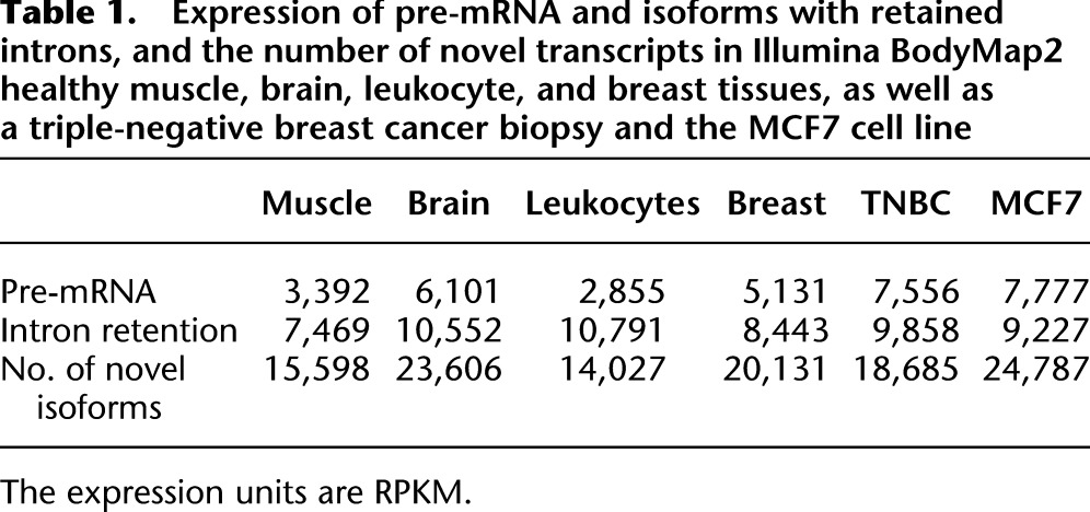
After validating the performance of iReckon on both simulated and real data, we used it to evaluate the splicing patterns in two cancer transcriptomes, especially to validate the method's ability to identify intron retention events. The two transcriptomes we consider are a triple-negative breast cancer (TNBC) patient sample recently sequenced at the BC Genome Sciences Center (Shah et al. 2012) and the MCF7 cell line (NCBI SRA accession SRX040504) (Sun et al. 2011). For comparative purposes, we also ran iReckon on additional data sets from the Illumina BodyMap2 data set, including muscle, brain, leukocytes, and breast. First, we evaluated the total amount of expressed pre-mRNA and intron retention identified in the various data sets, as well as the total number of novel isoforms (Table 1). While the total amount of intron retention or number of novel isoforms does not vary in a consistent fashion, the total amount of pre-mRNA observed was higher in the cancer transcriptome than in healthy tissues. This is generally supported by previous literature indicating overall inefficient splicing in some subtypes of cancer (Yoshida et al. 2011); however, variation in experimental protocols, cell subtypes, and interindividual variation cannot be easily excluded either.

Table 1.

Expression of pre-mRNA and isoforms with retained introns, and the number of novel transcripts in Illumina BodyMap2 healthy muscle, brain, leukocyte, and breast tissues, as well as a triple-negative breast cancer biopsy and the MCF7 cell line

In the following sections, we consider two intron retention events that have previously been reported in the cancer transcriptomes: the last intron of the NPC2 gene in the MCF7 cell line (Singh et al. 2011) and the seventh intron of the TP53 in the TNBC sample (Shah et al. 2012).

MCF7 transcriptome

In the study of Singh et al. (2011), the investigators identified and validated an intron retention event as well as an exon skipping event in the NPC2 gene. By running iReckon on this data set, we were able to detect both of these events, each of which is present in high abundance. RNA-seq reads alignment visualization with Savant and iReckon plugin (Fig. 5) confirms the findings. Furthermore, iReckon identified two additional alternative donor sites, leading to two novel isoforms: one alternative site within the exon, and one in the downstream intron. By use of the visualization plugin, we also detected a previously unknown single nucleotide variant (SNV) in the first nucleotide of the intron's donor site, changing the canonical GT to AT. The intron retention, the exon skipping, or the two alternative donor sites were not present in the TNBC data sets or in the Illumina healthy breast data set, and none of the events were found in the NCBI EST library. Thus, it is likely that the disruption of the canonical donor site of the last intron of the NPC2 gene results in several types of noncanonical splicing, including the following:

1. Intron entirely retained, resulting in an aberrant isoform;

2. Use of an alternative intra-exonic donor site 9 nucleotides (nt) upstream, resulting in the deletion of three amino acids from the coding region;

3. Use of an alternative donor site 16 nt downstream, resulting in an out-of-frame aberrant isoform; and

4. The skipping of the whole exon preceding the disrupted donor site, indicating that the splicing machinery failed because of unsuccessful exon recognition, rather than intron recognition (Berget 1995). The resulting mRNA product is also out-of-frame.

Figure 5.

Screen shot of Savant displaying a segment of the NPC2 gene in the MCF7 data set. (Red isoform) Exon skipping; (blue) intron retention; (green and yellow) contain the two alternative donor sites. The purple isoform with low expression is the pre-mRNA.

Table 2 presents the abundances of each of these isoforms, as well as the number of reads that can be uniquely assigned to each isoform.

Table 2.

Summary of detected isoforms of NPC2 in the MCF7 data set

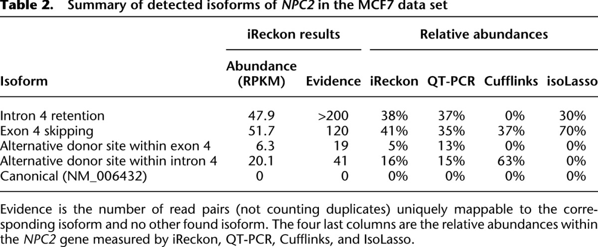
To validate iReckon's results, we performed QT-PCR with primers designed to detect each of the four isoforms (as well as the canonical one). All four isoforms were confirmed by QT-PCR, while the abundances observed closely matched those predicted by iReckon (see Table 2; r² = 0.94). The homozygous SNP that we detected disrupting the donor splice site (Fig. 5) was also confirmed by Sanger sequencing. For comparative purposes, we also ran Cufflinks and IsoLasso on this data set (we encountered technical issues with SLIDE) and noted that each of these methods missed two out of four novel isoforms (and predicted no additional ones).

TNBC transcriptome

While the MCF7 cell line consists exclusively of tumor cells, the TNBC transcriptome was taken from a patient biopsy and thus consists of a mixture of healthy and tumor material. Previously, Shah et al. (2012) uncovered a mutation in the acceptor site of intron 7 of TP53, mutating the canonical AG to GG and observed a correlated increase in the retention of the subsequent intron (computed using Miso) (Katz et al. 2010). The initial interpretation was that the mutation led to mis-splicing of the intron, leading to its retention.

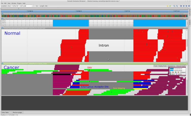
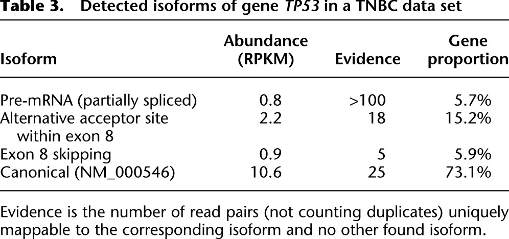
We evaluated this data set with iReckon and, surprisingly, did not predict the retention of intron 7. Instead, our method reported a significant presence of pre-mRNA, an alternative acceptor site used 19 bp downstream, as well as complete skipping of exon 8. All three of these events were found only in the TNBC data set and not in the healthy Illumina BodyMap2 breast or the MCF7 sample. These isoforms are shown in Figure 6.

Figure 6.

Savant screen shot showing healthy breast (from Illumina BodyMap2) and triple-negative breast cancer RNA-seq data. The third and fourth tracks display the aligned reads from healthy and cancer tissue, respectively, with the colors representing the isoform of origin. (Red isoform) Canonical annotated isoform. Its presence may be due to healthy cells biopsied together with the tumor. (Green isoform) Pre-mRNA (or partially spliced RNA); (blue) contains the alternative acceptor site; (yellow) skips the next exon (to the left since the transcript is on the reverse strand). We can also see the single nucleotide variant (SNV) that disrupted the acceptor site of the intron.

These results show that the consequences of a mutated acceptor site disruption are more complex than simply retaining the intron, and include the following:

1. An alternative intra-exonic acceptor site 19 nt downstream from the canonical site being used, creating an out of frame aberrant isoform.

2. The acceptor site of the next intron being used, resulting in exon skipping. The skipped exon length is not a multiple of three and creates an out of frame aberrant isoform.

3. The entire splicing mechanism becomes disrupted or slowed, resulting in the large abundance of partially spliced pre-mRNA with all four final introns retained in the transcript. If we consider the isoform corresponding to pre-mRNA and divide it into three segments, corresponding to introns 1–6, intron 7, and introns 8–10, the abundance estimates for these are 0.3, 2.4, and 2.5 RPKM, respectively. The coverage of the last four introns is thus consistent with disruption of splicing after the mutation, rather than the retention of a single intron.

Table 3 summarizes the abundances of these isoforms and the number of reads unambiguously mapped to each. All three events were only seen in the TNBC data set with this specific mutation and not in healthy breast or the MCF7 cell line. We expect TP53 mutations in TNBC to be early events in the evolutionary history of the tumor and therefore to be present in all (or the majority of) cells; however, the presence of multiple isoforms could result from either multiple aberrant transcripts within each cell, or the presence of multiple clonal populations in the sample. The relative quantity of TP53 pre-mRNA was higher in TNBC than in healthy breast and MCF7 (5.7% vs. 0.9% and 1.6% of the gene expression, respectively). Finally both the alternative acceptor site and the exon skipping event have not been previously reported in the NCBI EST library.

Table 3.

Detected isoforms of gene TP53 in a TNBC data set

Discussion

In this article, we introduce iReckon, a method for simultaneous isoform discovery and abundance estimation. iReckon models important biological phenomena such as intron retention and the presence of pre-mRNA. Our method generates a large set of possible isoforms and then utilizes a regularized EM algorithm to select expressed isoforms from these. Due to this particular approach and to the modeling of several RNA-seq artifacts (multimapping reads, PCR duplicates, biases) and biological mechanisms (pre-mRNA, intron retention), iReckon outperforms three popular current methods—Cufflinks, IsoLasso, and SLIDE—at both the identification of novel isoforms and the estimation of isoform abundances. We utilized iReckon to analyze the complexity of splicing profiles generated by the disruption of two canonical splice sites in a TNBC patient biopsy sample and the MCF7 cell line. In particular, we observed three or more different aberrant isoforms generated for both genes considered. The observed complexity of the splicing landscape raises important questions about the mechanisms involved and may lead to a better understanding of the underlying biology. The ability of iReckon to identify intron retention and pre-mRNA abundance may allow for novel biological discovery, for example, the pre-mRNA signal can be used to discern splicing order, as introns that are spliced-out later will be overrepresented in the pre-mRNA. Similarly, the analysis of intron retention can help uncover somatic mutations in cancer by identifying genes prone to aberrant splicing.

Finally we want to note that while iReckon outperforms other tools, there is still significant room for improvement. Even with simulated data, the top competing methods achieved overall recall of 62%, compared with 74% for iReckon; however, the numbers dropped significantly when one considers only novel isoforms: to 41% and 58%, respectively. Thus, nearly half of all novel isoforms are not being identified. Several steps can be taken to further improve the performance of iReckon. Perhaps the most important one is incorporation of sequencing biases, including those based on sequence content (e.g., GC rate) and location of a read within an isoform. Additional improvements can be achieved by directly modeling a wider variety of biological events. One such event, which may prove to be especially challenging, is the identification and abundance estimation of fusion genes. The performance of iReckon will also improve with development of better split-read mapping algorithms. Many of iReckon's false-negative isoforms in the simulation experiments (especially unidentified exon-skipping) were caused by splice junctions undiscovered by the initial alignment step.

Methods

Isoform reconstruction model extensions

In addition to modeling novel isoforms via paths in the splicing graph, as described in the Results section, iReckon also allows for two additional types of isoforms: pre-mRNA and isoforms with a retained intron.

Incorporating pre-mRNA

In real RNA-seq data, we observed that ∼1% − 30% of the RNA content for each gene can be due to unspliced pre-mRNA. While the exact percentage will vary due to gene regulation and sequence content, it is clear that treating pre-mRNA as noise can bias the results by leading to overestimation of isoform abundances (since some of the reads originally coming from pre-mRNA will be assigned to other isoforms) and can further complicate isoform reconstruction due to reads mapping across splice sites and into introns. To address this problem we add the complete pre-mRNA as a potential isoform for each gene predicted from the original reconstruction. This (unspliced) isoform's abundance is computed in the exact same manner as that of all other isoforms. Because these isoforms are only reported by our method, we do not consider these when evaluating the accuracy of the various tools.

Intron retention model

Incomplete pre-mRNA splicing can lead to intron retention events, where certain introns remain within mRNA that has undergone splicing. Transcripts with unspliced introns may affect cell function due to malformed proteins or haplo-insufficiency. Such intron retention events have been shown to play a role in certain cancers (Skotheim and Nees 2007; Kim et al. 2008; He et al. 2009). Note that intron retention cannot be accurately estimated if we do not take pre-mRNA into account, as reads from introns can be explained by either unspliced mRNA or intron retention.

We consider the null hypothesis H₀, that there is no intron retention, and all reads within introns come from unspliced pre-mRNA. To compute the P-value, we start by estimating the pre-mRNA abundance as the average coverage of introns. The isoform coverage signal at a nucleotide can be modeled by a Poisson(λ) distribution with the Poisson parameter being the average coverage (read locations are often modeled as Poisson variables, and the sum of Poisson variables is also Poisson). We compute the λ parameter for the pre-mRNA of each gene and reject the null hypothesis and detect an intron retention if an intron's coverage is statistically unlikely to be generated from the pre-mRNA (P-value < 10⁻⁴). Intron retention is a relatively rare event, so to reduce the computational complexity, iReckon considers only the one intron with the lowest P-value retained per gene. If we detect intron retention within a gene, we generate, for each isoform, a novel putative isoform with the corresponding intron retained within the mRNA and pass all these isoforms to the regularized EM algorithm.

Alignments and resulting optimizations

After constructing the set of all possible isoforms, we store their sequences in a transcriptome reference file (as opposed to a genome reference). We then use Burrows-Wheeler alignment (BWA) (Li and Durbin 2009) to align all the reads to the transcriptome, and from the possible alignments, we can compute read-isoform affinities for the nth read pair and the ith isoform as

where Q(n, i) is the mapping probability of the nth pair to the ith isoform computed from the alignment scores, L is the probability density function of the fragment length distribution within our RNA-seq experiment, and length(n,i) is the length of the fragment corresponding to the nth read pair if it originated from the ith isoform. These affinities are related to the compatibilities of Li et al. (2010) and Nicolae et al. (2011). The probability that the nth read pair, which aligns to the set of isoforms S_n, comes from the specific isoform of index i, of normalized abundance θ_i is computed as follows:

Z_ni is an indicator latent variable that is one if read pair n was generated from isoform i, and zero otherwise, and its expected value is .

Additionally, to improve the running time of the subsequent step, we separate all isoforms into independent groups, such that no read is mapped to isoforms in more than one group. Each of these groups can be processed separately by the regularized EM algorithm presented next, allowing for simple parallelizations and reducing memory usage. To further optimize the algorithm, we cluster the reads by their affinity signature. All the reads that align to the same subset of isoforms with very similar relative read–isoform affinities are clustered together and assigned to isoforms as a single entity, so that our algorithm only considers the affinities and cardinality of each cluster, instead of evaluating each read independently. We use a simple greedy clustering algorithm that unifies all pairs within a fixed distance of the center of the cluster. This heuristic has no observed influence over the performance of iReckon (recall, precision, quantification accuracy) while greatly improving its speed and reducing its memory usage. For clarity of presentation, we consider each read pair separately in the formulae below.

Regularized EM algorithm

Our method is an extension of previous EM-based approaches for transcript quantification (Li et al. 2010; Nicolae et al. 2011). The likelihood function for transcript abundance estimation with multimapped reads is very similar to the one introduced by Li et al. (2010):

Here r = (r₁, r₂,…, r_N) is the set of read-pairs and l = (l₁, l₂,…, l_M), θ = (θ₁, θ₂,…, θ_M) are, respectively, the lengths and abundances of the isoforms. z_n,i is the value of the Z_n,i latent indicator variable (see Equation 2). Finally, P(r_n|iso = i) is the probability that the read r_n is sampled from isoform i, and is constant with respect to the abundances θ.

As discussed previously, this algorithm may suffer from over-fitting. Because not all isoforms are expressed in a given sample, this problem is present even if only known isoforms are considered (Nicolae et al. 2011) and is exacerbated if the algorithm considers putative novel isoforms, most of which are likely to be false positives (Feng et al. 2011). Additional (unmodeled) biases and noise in the RNA-seq data further confound this, as extraneous predictors (isoforms) will be used to fit the noise and biases to increase the overall likelihood. Because our algorithm considers all plausible isoforms, it becomes crucial to introduce efficient regularization to remove false-positive isoforms by driving their expression to zero.

While the L1 penalty is commonly used as a solution to overfitting (e.g., Tibshirani 1996), it is not appropriate for abundance estimation. Because isoform abundances (in RPKM) are similar to normalized frequencies, they have positivity constraints as well as a fixed sum (see definition of RPKM):

The constant C is discussed in section 5 of the Supplemental Information. The regularization term minimized by LASSO is the sum of the abundances. However this term is tightly constrained, because abundances are very similar to frequencies. This type of regularization is not adequate in the hyperplane of the θ variables (described by the constraints). In order to reduce the number of nonzero abundances and thus avoid overfitting, we use a nonlinear function of the abundances in the penalty term. We have chosen the regularization penalty for its efficiency in giving sparse solutions (the fourth root is steep near zero) and its fast convergence speed. The specific shape of the function heavily penalizes low-abundance isoforms, while the penalty for high-abundance ones is lower. Adding regularization to the EM algorithm requires changes to the M step, as we can no longer directly solve the maximization problem. Hence we use a limited-memory Broyden–Fletcher–Goldfarb–Shanno (LBFGS) (Zhu et al. 1997) optimization algorithm for the M step, and because the objective function is no longer concave, we utilize random restarts to allow the EM algorithm to more fully explore the search space. The regularization rate λ is set so that most read pairs have affinity to an isoform with positive abundance. To do so, we iteratively increase lambda using progressively smaller steps until growing it any further would result in >0.01% of all reads not being assigned to an expressed isoform. We compared the performance using our regularization term, LASSO, and not doing regularization at all, and show that LASSO is inappropriate, while our method outperforms not doing regularization for most genes (see section 3 of the Supplemental Information).

The log-likelihood function that we optimize through the regularized EM algorithm is as follows:

where the first term is the data log-likelihood described above (with modifications to account for PCR Duplicates, described in the next section) and the second term is the regularization penalty. The third term (coherence score) is described fully in section 4 of the Supplemental Information. It is an additional parameter that allows the algorithm to further differentiate between multiple solutions with nearly identical likelihoods (for a full description of the isoform reconstruction ambiguity problem, see Lacroix et al. 2008). Because the regularization term deforms the final solution (abundances tend to become lower), our implementation contains a second step where we re-run the EM algorithm without regularization using only the isoforms with positive abundance in the optimal solution of Equation 5.

Accounting for PCR duplicates

Multiple rounds of PCR during the RNA-seq experiment can lead to multiple identical read pairs being generated from the same fragment. Either systematically removing or keeping all duplicates will bias the results. For example, in highly expressed genes, the observed duplicate reads may be natural duplicates (read pairs with identical locations generated from independent fragments), and removing them will cause underestimation of abundances. We estimate, for each read, its likelihood of being a PCR duplicate and use this probability in the objective function of the EM algorithm presented earlier (Equation 3).

First, we compute for each isoform the number of expected natural duplicates. Given an isoform with a known length l and abundance a, one can estimate the number of read pairs w that will be generated from this isoform. We treat w as the number of samples (fragments) drawn from the isoform. We estimate the probability p_f of a specific fragment f based on the isoform length, the fragment length distribution, and any biases (normalizing so that the probabilities of the different possible fragments sum to 1). The number of occurrences X_f of that particular fragment f is modeled by a binomial distribution B(w, p_f), which can be approximated by the Poisson (w × p_f) distribution since w is usually large (>20) and p_f is very small (<0.01). The number of duplicates of f is represented by the random variable Y_f = max{0, X_f − 1} corresponding to one “original read” and X_f − 1 copies. Y_f has the expected value

The derivation of this equation is presented in the Supplemental Information. The total expected number of natural duplicates is the sum of the expectations over the possible fragments:

where F_s is the set of fragments starting at position s that can possibly be originated from the studied isoform.

For each read r_n, we now calculate the probability P(d_n = 1), d_n being the indicator variable that is zero when the read is a PCR duplicate. For the ith isoform, let Nb_Copies_i be the observed number of duplicates and Nb_Natural_i the number of expected natural duplicates (computed in Equation 7). Then

where S_n is the set of isoforms the read r_n aligns to, and is the alignment probability based on Equation 2. The EM likelihood function presented earlier (Equation 3) can thus be updated to properly account for PCR duplicates by adding the indicator variable d_n:

Because small changes in abundances do not significantly affect duplicate estimation, we do not need to update the probabilities at every iteration of the EM algorithm. For efficiency, we update these only when the abundances have changed significantly from their previous values.

RNA-seq data simulation

To simulate a realistic data set with known ground truth, we randomly selected 75% of the multi-exonic isoforms of the UCSC refGene data set to study and, for each of these, generated a set of alternative splicing events: exon skipping and intron retention. Each exon had 10% chance to be skipped, and the skipping could be extended to the following exons with 30% probability per exon, while each intron was retained with 1.8% probability. These probabilities were adjusted based on the number of exons in the gene and based on the number of alternative isoforms already simulated. We then selected multiple random subsets of all events to be implanted in the original isoform. Finally, we add to this set of isoforms the pre-mRNAs of all studied genes.

This set of isoforms is then given to FluxSimulator (The FluxProject 2011), which randomly orders these and picks an abundance for each following a mixed power/exponential law. The parameters from the law were chosen so that the range of the isoforms' expression is 10⁴ (the highest abundance over the lowest). While FluxSimulator assigned a random abundance to the pre-mRNA, we adjusted this to 10% of the initial value to correspond to the expected low abundance of such isoforms. FluxSimulator was then used to simulate RNA-seq read pairs from these isoforms in a manner that reproduces in silico the experimental pipelines for RNA-seq, making the simulated data sets as realistic as possible.

The results presented here are obtained from a simulation with 1615 genes, 8 million read pairs, and 3539 isoforms, of which 30% are novel (pre-mRNAs are not counted). We also conducted three additional simulations with slightly different parameters (number of reads, proportion of novel isoforms, etc.), but no significant change was observed in the results of the comparison between iReckon and the other methods (data not shown).

Program performance

iReckon required 22 h to complete on the Illumina BodyMap2 muscle data set (contains ∼82 × 10⁶ pairs of 50-bp-long reads), using an eight-core machine with 32-GB RAM (the actual memory usage maxed at ∼9 GB) and 80 GB of local storage. The largest component of the running time (10 h) is the alignment of reads to isoforms using BWA.

Software availability

iReckon is available both as a standalone package (open source), which can be downloaded from http://compbio.cs.toronto.edu/ireckon, and as a plugin for the Savant Genome Browser (Fiume et al. 2010, 2012), which enables running iReckon on individual genes in real-time.

References

- Berget S 1995. Exon recognition in vertebrate splicing. J Biol Chem 270: 2411. [DOI] [PubMed] [Google Scholar]
- Bohnert R, Rätsch G 2010. rQuant.web: A tool for RNA-seq-based transcript quantitation. Nucleic Acids Res (suppl 2) 38: W348–W351 [DOI] [PMC free article] [PubMed] [Google Scholar]
- Feng J, Li W, Jiang T 2011. Inference of isoforms from short sequence reads. J Comput Biol 18: 305–321 [DOI] [PMC free article] [PubMed] [Google Scholar]
- Fiume M, Williams V, Brook A, Brudno M 2010. Savant: Genome browser for high-throughput sequencing data. Bioinformatics 26: 1938–1944 [DOI] [PMC free article] [PubMed] [Google Scholar]
- Fiume M, Smith E, Brook A, Strbenac D, Turner B, Mezlini A, Robinson M, Wodak S, Brudno M 2012. Savant genome browser 2: Visualization and analysis for population-scale genomics. Nucleic Acids Res 40: W615–W621 [DOI] [PMC free article] [PubMed] [Google Scholar]
- The FluxProject. 2011. 2011 FluxSimulator v1.0.RC4. http://flux.sammeth.net.
- He C, Zhou F, Zuo Z, Cheng H, Zhou R 2009. A global view of cancer-specific transcript variants by subtractive Transcriptome-Wide analysis. PLoS ONE 4: e4732. [DOI] [PMC free article] [PubMed] [Google Scholar]
- Heber S, Alekseyev M, Sze S, Tang H, Pevzner PA 2002. Splicing graphs and EST assembly problem. Bioinformatics 18: S181–S188 [DOI] [PubMed] [Google Scholar]
- Katz Y, Wang E, Airoldi E, Burge C 2010. Analysis and design of rna sequencing experiments for identifying isoform regulation. Nat Methods 7: 1009–1015 [DOI] [PMC free article] [PubMed] [Google Scholar]
- Kim E, Goren A, Ast G 2008. Insights into the connection between cancer and alternative splicing. Trends Genet 24: 7–10 [DOI] [PubMed] [Google Scholar]
- Lacroix V, Sammeth M, Guigo R, Bergeron A 2008. Exact transcriptome reconstruction from short sequence reads. In Algorithms in bioinformatics, Vol. 5251, Lecture notes in computer science (ed. K Crandall and J Lagergren), pp. 50–63. Springer, Berlin/Heidelberg [Google Scholar]
- Li H, Durbin R 2009. Fast and accurate short read alignment with Burrows–Wheeler transform. Bioinformatics 25: 1754–1760 [DOI] [PMC free article] [PubMed] [Google Scholar]
- Li H, Zhang K, Jiang T 2005. The regularized EM algorithm. In Proceedings of the 20th national conference on artificial intelligence, Vol. 2, pp. 807–812. AAAI Press, Menlo Park, CA [Google Scholar]
- Li B, Ruotti V, Stewart RM, Thomson JA, Dewey CN 2010. RNA-seq gene expression estimation with read mapping uncertainty. Bioinformatics 26: 493–500 [DOI] [PMC free article] [PubMed] [Google Scholar]
- Li J, Jiang C, Brown J, Huang H, Bickel P 2011. Sparse linear modeling of next-generation mRNA sequencing (RNA-Seq) data for isoform discovery and abundance estimation. Proc Natl Acad Sci 108: 19867–19872 [DOI] [PMC free article] [PubMed] [Google Scholar]
- Li W, Feng J, Jiang T 2011. IsoLasso: A LASSO regression approach to RNA-seq based transcriptome assembly. In Research in computational molecular biology, Vol. 6577, Lecture notes in computer science (ed. V Bafna and S Sahinalp), pp. 168–188. Springer, Berlin/Heidelberg [Google Scholar]
- Lopezbigas N, Audit B, Ouzounis C, Parra G, Guigo R 2005. Are splicing mutations the most frequent cause of hereditary disease? FEBS Lett 579: 1900–1903 [DOI] [PubMed] [Google Scholar]
- McLachlan G, Peel D 2000. Finite mixture models, Vol. 299. Wiley-Interscience, Hoboken, NJ [Google Scholar]
- Nicolae M, Mangul S, Mandoiu I, Zelikovsky A 2011. Estimation of alternative splicing isoform frequencies from RNA-seq data. Algorithms Mol Biol 6: 9. [DOI] [PMC free article] [PubMed] [Google Scholar]
- Shah S, Roth A, Goya R, Aparicio S 2012. The clonal and mutational evolution spectrum of primary triple negative breast cancer. Nature 7: 1009–1015 [DOI] [PMC free article] [PubMed] [Google Scholar]
- Singh D, Orellana C, Hu Y, Jones C, Liu Y, Chiang D, Liu J, Prins J 2011. Fdm: A graph-based statistical method to detect differential transcription using rna-seq data. Bioinformatics 27: 2633–2640 [DOI] [PMC free article] [PubMed] [Google Scholar]
- Skotheim RI, Nees M 2007. Alternative splicing in cancer: Noise, functional, or systematic? Int J Biochem Cell Biol 39: 1432–1449 [DOI] [PubMed] [Google Scholar]
- Sun Z, Asmann Y, Kalari K, Bot B, Eckel-Passow J, Baker T, Carr J, Khrebtukova I, Luo S, Zhang L, et al. 2011. Integrated analysis of gene expression, cpg island methylation, and gene copy number in breast cancer cells by deep sequencing. PLoS ONE 6: e17490. [DOI] [PMC free article] [PubMed] [Google Scholar]
- Tibshirani R 1996. Regression shrinkage and selection via the lasso. J R Stat Soc Ser B Methodol 58: 267–288 [Google Scholar]
- Trapnell C, Pachter L, Salzberg SL 2009. TopHat: Discovering splice junctions with RNA-seq. Bioinformatics 25: 1105–1111 [DOI] [PMC free article] [PubMed] [Google Scholar]
- Trapnell C, Williams BA, Pertea G, Mortazavi A, Kwan G, van Baren MJ, Salzberg SL, Wold BJ, Pachter L 2010. Transcript assembly and quantification by RNA-seq reveals unannotated transcripts and isoform switching during cell differentiation. Nat Biotechnol 28: 511–515 [DOI] [PMC free article] [PubMed] [Google Scholar]
- Wang Z, Gerstein M, Snyder M 2009. RNA-seq: A revolutionary tool for transcriptomics. Nat Rev Genet 10: 57–63 [DOI] [PMC free article] [PubMed] [Google Scholar]
- Wang K, Singh D, Zeng Z, Coleman SJ, Huang Y, Savich GL, He X, Mieczkowski P, Grimm SA, Perou CM, et al. 2010. MapSplice: Accurate mapping of RNA-seq reads for splice junction discovery. Nucleic Acids Res 38: e178. [DOI] [PMC free article] [PubMed] [Google Scholar]
- Yoshida K, Sanada M, Shiraishi Y, Nowak D, Nagata Y, Yamamoto R, Sato Y, Sato-Otsubo A, Kon A, Nagasaki M, et al. 2011. Frequent pathway mutations of splicing machinery in myelodysplasia. Nature 478: 64–69 [DOI] [PubMed] [Google Scholar]
- Zhu C, Byrd RH, Lu P, Nocedal J 1997. Algorithm 778: L-BFGS-B: Fortran subroutines for large-scale bound-constrained optimization. ACM Trans Math Softw 23: 550–560 [Google Scholar]