Abstract
The field of view (FOV) of a cone-beam computed tomography (CBCT) unit in single-photon emission computed tomography (SPECT)/CBCT system can be increased by offsetting CBCT detector. Analytic-based algorithms have been developed for image reconstruction from data collected at a large number of densely sampled views in offset-detector CBCT. However, the radiation dose involved in a large number of projections can be of a health concern to the imaged subject. CBCT-imaging dose can be reduced by lowering the number of projections. As analytic-based algorithms are unlikely to reconstruct accurate images from sparse-view data, we investigate and characterize in the work optimization-based algorithms, including an adaptive steepest descent-weighted projection onto convex sets (ASD-WPOCS) algorithm, for image reconstruction from sparse-view data collected in offset-detector CBCT. Using simulated data, and real data collected from a physical pelvis phantom and patient, we verify and characterize properties of the algorithms under study. Results of our study suggest that optimization-based algorithms such as ASD-WPOCS may be developed for yielding images of potential utility from a number of projections substantially smaller than those used currently in clinical SPECT/CBCT imaging, thus leading to a dose reduction in CBCT imaging.
I. Introduction
In recent years, combined single-photon emission computed tomography (SPECT) and cone-beam computed tomography (CBCT) systems have been developed and become available commercially [1]–[6] for yielding functional and anatomic information about an imaged subject. CBCT images can also be used to compensate for attenuation artifacts in SPECT images. The CBCT unit in a SPECT/CBCT system developed recently uses a flat-panel detector of a limited size due to cost and hardware considerations [6], [7]. In an attempt to increase the field of view (FOV) of CBCT, one can offset the flat-panel detector to form an asymmetric coverage of the imaged object at each view [8]. Analytic-based algorithms have been developed for image reconstruction from data collected with an offset-detector configuration [9]. However, the algorithms generally require data collected at a large number of densely distributed views.
CBCT scans promise added-on value to SPECT imaging through offering information about patient anatomy and for attenuation correction in SPECT; however, radiation dose involved in CBCT scans constitutes a potential health concern to the imaged subject. For a given X-ray flux level, CBCT-imaging dose can be reduced by decreasing the number of views at which projections are acquired. Analytic-based algorithms are unlikely to reconstruct accurate images from sparse-view data as they are designed to work only for densely sampled data. On the other hand, it has been demonstrated that optimization-based algorithms may reconstruct images of potential utility from projections much fewer than those required by analytic-based algorithms [10]–[13]. There exists a significant interest in image reconstruction from sparse-view projections in both industry and academia [14]–[20].
In this work, we investigate and characterize image reconstruction from data, and particularly from sparse-view data, collected in offset-detector CBCT. We also clarify issues concerning data redundancy and imaging-model linearity involved in analytic- and optimization-based algorithms. Using simulated data, and real data collected from a physical pelvis phantom [21] and patient, we verify and characterize the algorithms under study.
We organize the paper as follows: Sec. II describes imaging configuration and data acquisition in offset-detector CBCT; Secs. III–V summarize, and contrast, the development of imaging models, reconstruction programs, and weighting schemes for analytic- and optimization-based algorithms, followed by inverse-crime studies [22]–[24] in Secs. VI and VII for validating the algorithms; Sec. VIII reports studies involving real data of a physical pelvis phantom and patient for characterizing algorithm properties; and finally, Secs. IX and X narrate discussions and conclusions of the study.
II. Parameters for Offset-detector CBCT Imaging
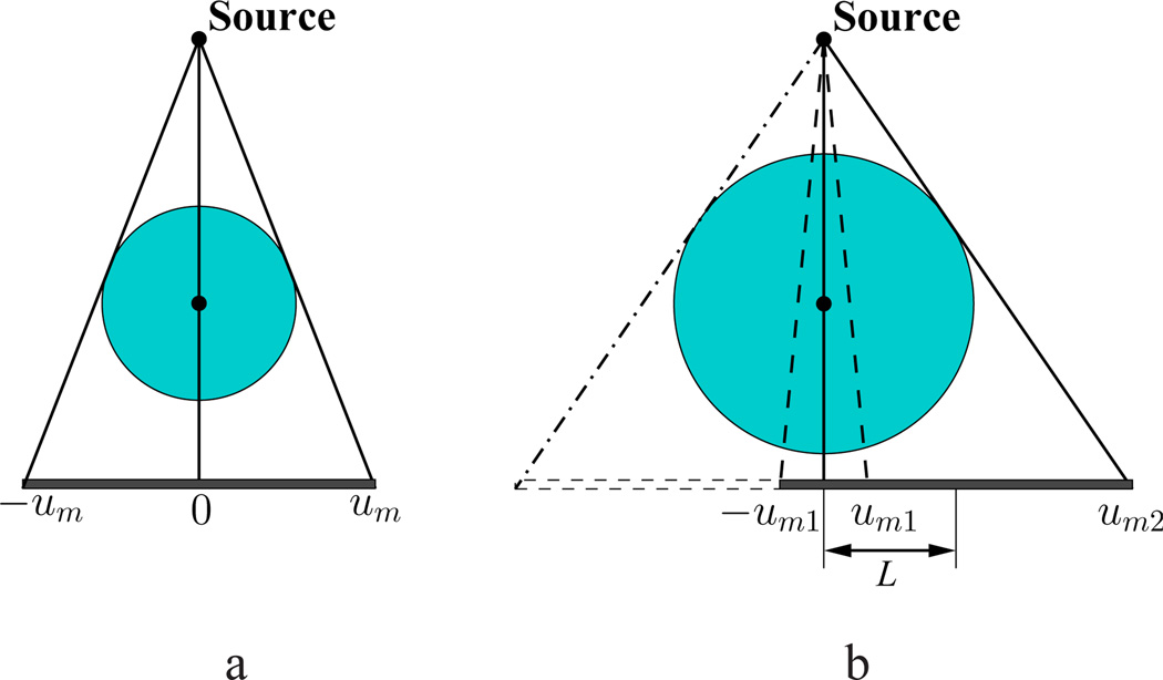
Clinical SPECT/CBCT uses a circular scanning trajectory for data collection. We refer to the plane containing the circular trajectory as the middle plane, and to other planes parallel to the middle plane as non-middle planes. As shown in Fig. 1, CBCT imaging configuration within the middle plane constitutes a fan-beam geometry. We define central lines at each view as the lines connecting the source and rotation axis, and assume that the central line within the middle plane is perpendicular to the detector plane, thus forming an FOV shown in Fig. 1a. It is well-known [8], [9] that a CBCT FOV can be expanded effectively by offsetting the detector within the detector plane along a direction perpendicular to the rotation axis. Let um and υm denote halves of the detector sizes perpendicular to, and along, the rotation axis. For offset length L, we define um1 = um −L and um2 = um+L, where L < um, and display the extended FOV in Fig. 1b. For a fan-beam offset-detector geometry shown in Fig. 1b, projections between −um1 and um1 are measured twice, while projections between um1 and um2 are collected only once, as the source/detector rotates over 2π. Therefore, data acquired with a fan-beam offset-detector geometry is partially redundant, and are sufficient for accurate reconstruction within the middle plane.
Figure 1.
Fields of view (FOVs) formed by a non-offset detector of size 2um (a) and by an offset detector (b) within the middle plane. The rotation axis, perpendicular to the middle plane is indicated as black dots at the centers of the circular FOVs. L denotes the offset length, um1 = um − L, and um2 = um + L.
We use the offset-detector CBCT unit of a SPECT/CT system (BrightView XCT, Philips) to collect data in the study. The X-ray source and flat-panel detector, along with the SPECT unit, are mounted on a gantry, and form a circular trajectory when the gantry rotates. The distances of the X-ray source to the detector plane and to the center of rotation are 133.2 cm and 88.1 cm. The detector panel with a size of 40 × 30 cm2 consists of 2048×1536 elements each of which has a size of 0.194×0.194 mm2. In clinical applications, the detector is used under a 2×4-binning mode, thus resulting in 1024×384 rectangle-shaped, effective elements of 0.388×0.776 mm2 size. Let um = 20 cm and υm = 15 cm denote half sizes of the detector. An offset L = 17.7 cm is considered for expanding the FOV to a size of about 48 cm (axial)×15 cm (transaxial) shown in Fig. 1b. In clinical SPECT/CT, data at 720 views uniformly distributed over 2π are acquired with a circular trajectory, followed by correction for background, uniformity, detector-gain mode, and defective pixels, as well as physical factors such as scatter and beam hardening. In the work, data were collected at 720 views uniformly distributed over 2π from a physical pelvis phantom and patient. Throughout the work, we refer to 720-view data as full data.
In real-data studies below, considering the rectangular shape of an effective detector element, we reconstructed images on 600 × 840 × 175 and 600 × 840 × 164 arrays of prism-shaped voxels (instead of cube-shaped voxels) for the physical pelvis phantom and patient. The transverse and longitudinal sizes of each prism were 0.05 cm and 0.1 cm.
III. Analytic-based image reconstruction
The focus of the study is on optimization-based image reconstruction from sparse-view data collected with offset-detector CBCT. However, the FDK algorithm [25], an analytic-based algorithm used widely in practical applications, serves as a reference for characterization of optimization-based reconstructions. In an attempt to contrast the key components involved in optimization-based reconstructions, we describe briefly below the counterparts involved in analytic-based image reconstruction, even though many of them are generally well-known.
A. Continuous-to-continuous imaging model
Analytic-based algorithms are developed based upon a linear, continuous-to-continuous (C-C) imaging model in which a CBCT measurement is interpreted as a line integral of an object function:
| (1) |
where g0(u, υ, λ) denotes continuous model data at a point (u, υ) on the detector plane from view λ; f(r) is the object function at a point specified by r in the image space; r0(λ) is the source location outside the object support at view λ; and θ̂(u, υ, λ) is a unit vector originating from r0(λ) and pointing to (u, υ) on the detector plane. In a C-C imaging model, variables u, υ, and λ and r can vary continuously in the data and image spaces.
B. Analytic-based reconstruction programs
For certain conditions, reconstruction programs (or, equivalently, inversion formulas) can be derived [26]–[30] in which the object function can be expressed explicitly in terms of the data function. The programs can be used for determining data conditions sufficient for yielding mathematically exact solutions to the C-C imaging model in Eq. (1). For example, a reconstruction program derived by Tuy [26] has been used widely for determining data sufficiency conditions. Although some of the programs involve data or data transformations that are practically impossible to achieve, thus preventing them from being used directly as reconstruction algorithms, they can be used as the basis for the derivation of analytic-based algorithms that can be practically implementable. For example, for certain imaging configurations, based upon the Tuy’s reconstruction program, a filtered-backprojection (FBP) algorithm [27] can be derived, whereas based on the reconstruction program in Eq. (9) of Ref. [28], a backprojection-filtration (BPF) algorithm [30] can be derived.
C. Analytic-based reconstruction algorithms
Analytic-based algorithms can be derived for solving exactly the C-C imaging model in Eq. (1) for helical and other scanning configurations that satisfy Tuy’s data-sufficiency condition [27]–[30]. For a circular configuration, which is often used for data acquisition in practical CBCT, the algorithms can offer an exact reconstruction only for the middle plane, and approximate reconstructions for non-middle planes, because only the middle plane satisfies Tuy’s data-sufficiency condition whereas non-middle planes do not. The FDK algorithm considered in the work is an FBP-type algorithm that offers exact and approximate reconstructions, respectively, to the middle and non-middle planes.
1) Discrete approximation
Analytic-based algorithms for solving exactly, or approximately, Eq. (1), are for object and data functions in continuous forms. Because only discrete data can be collected in practical CBCT imaging, discrete forms of analytic-based algorithms have to be devised for accommodating discrete data. An analytic-based algorithm in a discrete form generally provides only an approximate inversion to the C-C imaging model, even if the algorithm in its continuous form exactly solves Eq. (1). An analytic-based algorithm in different discrete forms thus yields numerically different reconstructions [31], [32]. For the middle plane, the FDK algorithm in a discrete form provides an approximate solution due to algorithm discretization, whereas, for non-middle planes, the FDK algorithm in a discrete form offers an approximate solution due to both data insufficiency and algorithm discretization.
2) Data redundancy
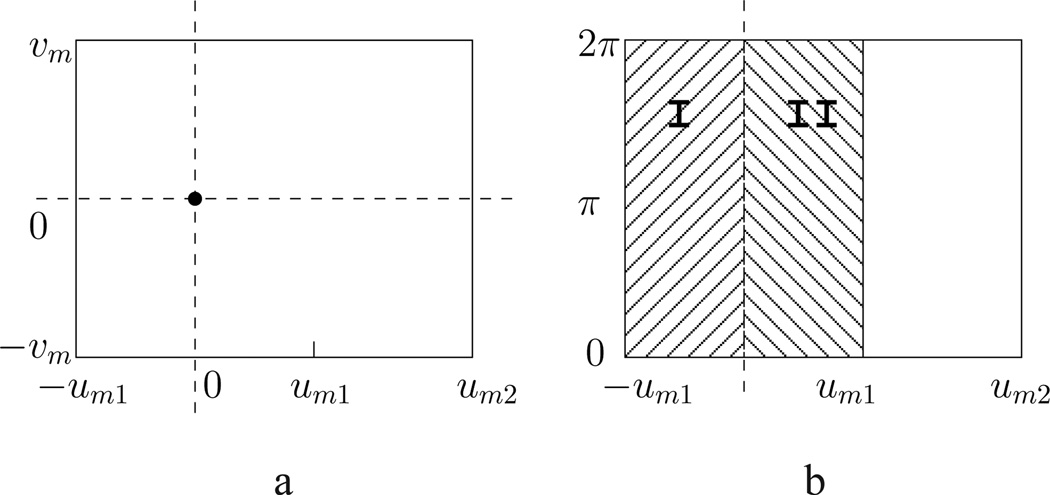
We show in Fig. 2a a flat-panel detector offset by L viewing from the source. A sinogram can also be formed with a detector row from all of the views over 2π, as illustrated in Fig. 2b. Data collected over 2π with a detector row specified by υ = 0 (i.e., from the middle plane) contain partially redundant information because there are pairs of X-rays collected that coincide with each other. Such partial data redundancy has to be normalized with a weighting function [33] so that analytic-based algorithms can be applied. Mathematically, circular CBCT data collected with a detector row specified by υ ≠ 0 contain no redundant information, because none of the collected X-rays coincide with each other. However, for two X-rays within a plane that contains a pair of coinciding X-rays in the middle plane and that is perpendicular to the middle plane, they are considered approximately redundant if the two X-rays have identical cone angles. A weighting function selected for the detector row specified by υ = 0 is used also as the weighting functions for detector rows specified by υ ≠ 0.
Figure 2.
(a) An offset detector plane in which the horizontal, and vertical, dashed lines denote the projections of the rotation axis onto, and the intersection of the middle plane with, the detector. (b) Sinogram space formed by a detector row specified by υ over 2π. For the detector row specified by υ = 0, continuous model data in regions I and II are redundant; whereas for detector row specified by υ ≠ 0, model data in regions I and II are only approximately redundant.
IV. Optimization-based Image Reconstructions
Optimization-based reconstruction also entails key components similar to those in analytic-based reconstruction: imaging model, reconstruction program, and reconstruction algorithm, which we discuss below.
A. Discrete-to-discrete imaging model
In optimization-based reconstruction, a linear discrete-to-discrete (D-D), instead of a linear C-C, model is used for summarizing the CBCT imaging process
| (2) |
where ℋ is an M × N system matrix modeling the cone-beam X-ray transform; vectors g0 and f of sizes M and N denote discrete model data and discrete image to be reconstructed. Each entry of g0 or f denotes a model-data value within an effective detector element or an image value within a voxel. In practice, measured data g of size M differ than model data g0 and consists of entries denoting measured data values.
Reconstruction of image f is equivalent to inverting the linear system in Eq. (2) from knowledge of measured, discrete data. Although a D-D imaging model can be devised based upon a C-C imaging model, an analytic-based algorithm solving exactly the C-C imaging model cannot invert exactly the D-D imaging model even if the algorithm is in a discrete form. In realistic CBCT applications, the D-D imaging model in Eq. (2) involves a huge-size matrix that prevents its direct inversion. Instead, optimization-based algorithms are used for solving the D-D imaging model.
B. Optimization-based reconstruction programs
Based upon Eq. (2), an optimization program has been developed [10]–[13] for CBCT-image reconstruction in which the image total-variation (TV) (i.e., the ℓ1-norm of the gradient magnitude image) is minimized, subject to constraints on data fidelity and image positivity. Using this optimization program, we devise reconstruction program 1 for image reconstruction specifically from data collected in offset-detector CBCT. For a performance comparison to reconstruction program 1 and its corresponding algorithm, we also consider reconstruction program 2 based on Kullback-Leibler (KL) divergence [34] and the corresponding expectation-maximization (EM) algorithm [34]–[36] for offset-detector CBCT. We describe the two optimization-based reconstruction programs below.
1) Reconstruction program 1
The first reconstruction program [37] is written as:
| (3) |
where D𝒲(f) denotes a weighted Euclidean data divergence between the measured data and model data:
| (4) |
where 𝒲 is an M × M diagonal matrix in which each diagonal element represents a positive weighting factor for a particular X-ray measured; ‖f‖TV the image TV; fj image value at voxel j, j = 1, 2, …, N; cα(f) (defined in Eq. (21) of Ref. [11]) can be calculated for each f, and cα(f) → −1 provides a necessary condition on algorithm convergence [11], [12]. Parameter ε > 0 determines a level of allowable average inconsistency between the measured data and model data per effective detector element; parameter t0 > 0 provides a lower bound for the image TV; and parameter γ should be larger than, but close to, −1. The reconstruction program therefore designs a solution set.
2) Reconstruction program 2
One can rewrite Eq. (2) as
| (5) |
where and ℋ′ = 𝒲ℋ. Defining g′ = 𝒲g and using Eq. (5), we devise reconstruction program 2 as
| (6) |
where DKL(f) denotes the KL divergence between g′ and ℋ′f [34]; and parameter εKL > 0 specifies a lower bound for the KL divergence. Again, the reconstruction program determines another solution set, which can differ from that specified by reconstruction program 1.
3) Program parameters
Reconstruction programs 1 and 2 are specified not only by explicit parameters, including ε, t0, γ, εKL, and 𝒲, but also by implicit attributes such as basis sets spanning the image and data spaces and a specific method for calculating the system matrix ℋ. Different selections of these parameters and attributes, which are referred to as program parameters in this work, necessarily result in different sets of designed solutions (or, equivalently, designed reconstructions). In this work, prism-shaped voxels and rectangle-shaped pixels were used for spanning the image and data spaces, whereas intersection length of an X-ray with an image voxel is selected as an element of system matrix ℋ [11]–[13]. We also discuss in numerical studies in Sec. V below the selection of program parameters such as the weighting matrices for reconstruction tasks considered.
C. Optimization-based reconstruction algorithms
We describe below algorithms that numerically solve reconstruction programs 1 and 2.
1) ASD-WPOCS algorithm for reconstruction program 1
The existing ASD-POCS algorithm [10], [11] can be used for image reconstruction through solving program 1. However, as numerical studies demonstrated (see Fig. 8 below), the POCS method [38]–[40] that lowers D𝒲(f) can result in image artifacts in the presence of data inconsistencies. Therefore, we consider a weighted POCS (WPOCS) algorithm:
| (7) |
where f(n,i) denotes reconstruction at the n-th iteration after the updates from the i-th equation; Hi the i-th row vector of the system matrix ℋ; 0 < β < 2 is a relaxation factor; gi the i-th entry in the measured data g; 𝒲ii the i-th diagonal element of 𝒲, which is chosen to be 0 < 𝒲ii ≤ 1 in this work; and i = 1, 2, …, M.
Figure 8.
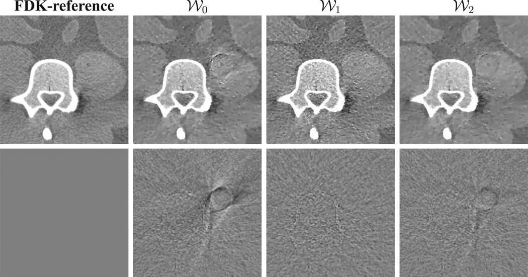
Row 1: FDK-reference ROI image and ROI images reconstructed by use of ASD-WPOCS algorithm with weighting matrices 𝒲0, 𝒲1, and 𝒲2 from real data of the physical pelvis phantom. Display window: [0.1, 0.25] cm−1. Row 2: Differences between ROI images in row 1 and the FDK-reference ROI image. Display window: [−0.05, 0.05] cm−1.
We refer to this algorithm as the ASD-WPOCS algorithm, in which we use the steepest descent (SD) and WPOCS methods to lower adaptively ‖f‖TV and D𝒲(f) until they reach the preselected values [10]–[13]. The pseudocode implementing the ASD-WPOCS is identical to that for the ASD-POCS described in Refs. [10], [11], except for that the POCS step is replaced by the WPOCS step and data divergence is replaced by D𝒲(f). For a given set of parameters ε, t0, γ, and 𝒲, when D𝒲(f) ≤ ε is achieved, we then use a gradient descent method, instead of the WPOCS method, for further lowering D𝒲(f) until ‖f‖TV ≤ t0 and cα(f) ≤ γ are satisfied [10]–[13]. In this work, an initial image f = 0 is used in the ASD-WPOCS reconstruction.
2) EM algorithm for reconstruction program 2
The EM algorithm [34]–[36] can be used for minimizing the KL divergence in Eq. (6). In the presence of 𝒲, it can readily be shown that KL-divergence DKL(f) can be minimized by use of the EM algorithm:
| (8) |
where denotes the j-th voxel value at iteration n; and ℋij is the element of system matrix ℋ at the i-th row and j-th column, 𝒲ii > 0, i = 1, 2, …, M, and j = 1, 2, …, N. An initial image f = 1 was used in EM reconstruction.
V. Selection of weighting functions and matrices
A. Weighting functions for the C-C imaging model
For demonstrating the effect of weighting functions on analytic-based reconstructions, we carried out a reconstruction directly from data without weighting (or, equivalently, with an identity weighting). For convenience, we write the identity weighting function as
| (9) |
and W0(u, υ, λ) = 0 for −um2 < u ≤ −um1, where |υ| ≤ υm.
One can also devise a weighting function to normalize data redundancy. As shown in Fig. 2b, continuous data g0(u, 0, λ), collected with a detector row indexed by υ = 0, in regions I and II are redundant, and can be normalized by a weighting function satisfying W(u, 0, λ) + W(−u, 0, λ) = 1, for 0 ≤ u ≤ um1, W(u, 0, λ) = 0 for −um2 < u ≤ −um1, and W(u, 0, λ) = 1 for um1 < u ≤ um2. The same weighting function is used also for normalizing the approximate data redundancy for non-middle planes. i.e., W(u, υ, λ) = W(u, 0, λ), where |υ| ≤ υm.
We consider two weighting functions satisfying the normalization condition:
| (10) |
and
| (11) |
where |υ| ≤ υm, , and S is the source-to-detector distance, and W1(u, υ, λ) = W2(u, υ, λ) = 0 for −um2 < u ≤ −um1 and 1 for um1 < u ≤ um2.
It can be observed that W1 is a smooth function of u, but W0 and W2 are not. The weighting functions have to be discretized when they are applied to measured, discrete data, thus becoming approximate weighting functions with respect to data redundancy in the C-C imaging model. The weighting functions in their discrete forms can impact on reconstruction quality.
B. Selection of weighting matrices for the D-D imaging model
Model data g0, as well as measured data g, generally contain no redundant information, because no rows in the system matrix ℋ are identical. Therefore, the multiplication of an appropriately selected weighting matrix to both sides of a linear D-D imaging model cannot be interpreted as data-redundancy normalization. Instead, it is a consequence of the linearity property of a D-D imaging model. Different weighting matrices result in different D𝒲(f) and thus different reconstruction programs, resulting in different reconstructions when data are inconsistent with the D-D imaging model. This property can be exploited for potentially improving image reconstructions by devising appropriate weighting matrices.
In the work, we considered three diagonal weighting matrices that are formed, respectively, from the three weighting functions of Eqs. (9)–(11) in their discrete forms. Specifically, each of the three discrete weighting functions is written in a concatenated form to compose diagonal elements of a weighting matrix for the D-D imaging model. We refer to weighting matrices formed with discrete weighting functionsW0, W1, and W2 as weighting matrices 𝒲0, 𝒲1, and 𝒲2, respectively. The weighting matrices will be used for computing D𝒲(f) in Eq. (4) and in the WPOCS and EM algorithms of Eqs. (7) and (8).
VI. Studies based on the C-C imaging model
Using inverse-crime studies [22]–[24] in which data are consistent with the imaging model, we can verify if the reconstruction algorithms solve the corresponding reconstruction program. Using numerical studies in which data are inconsistent with the imaging model, we can also characterize the numerical properties of the reconstruction algorithms. The FDK algorithm considered in the work has been verified and characterized previously. We summarize briefly the inverse-crime and numerical studies of the FDK algorithm even though they are already well-known for the purpose of contrasting the studies in Secs. VII and VIII for the verification and characterization of optimization-based algorithms.
A. Inverse-crime studies
For an offset-detector scanning over a circular trajectory, we can plug in the FDK algorithm with normalization weighting functions W1 or W2 into the C-C model specified by Eq. (1). It can be readily shown that the FDK algorithm yields a mathematically exact, explicit solution to the C-C imaging model for the middle plane. This constitutes an inverse-crime study for verification of the FDK algorithm. For the non-middle planes, the FDK algorithm only yields an approximate solution to the C-C model.
B. Real-data studies
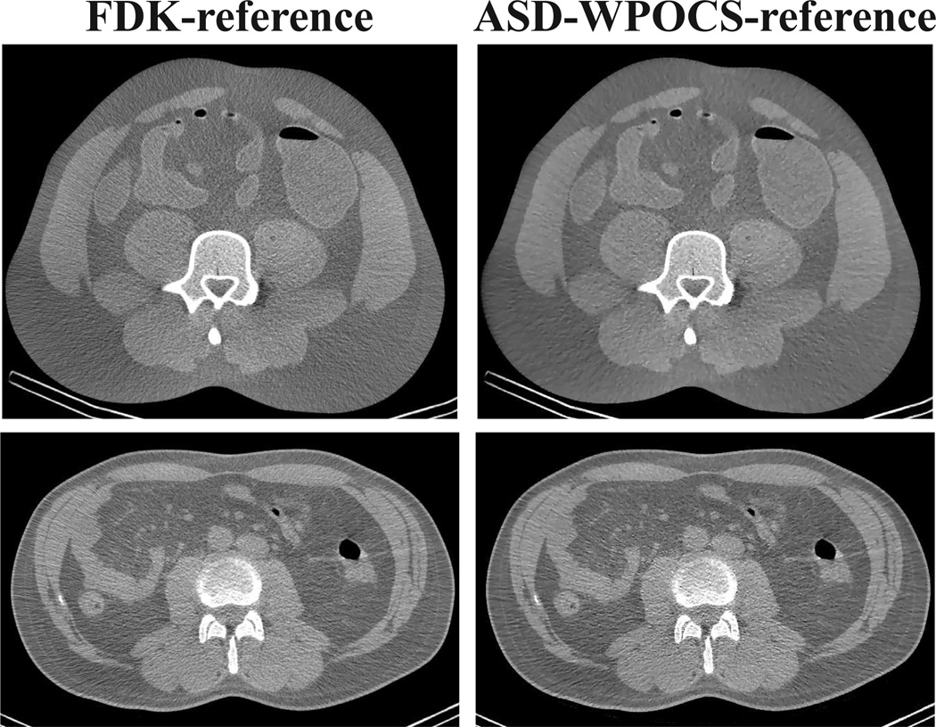
The property of the FDK algorithm can also be characterized by use of real, discrete data that are inconsistent with the C-C imaging model. Existing studies demonstrate that smooth weighting functions such as W1 can yield images with minimized artifacts [9], [33]. Therefore, we used W1 as the weighting function in the study. We first normalized 720-view data of a pelvis phantom or patient, as described in Sec. VIII, by using discrete-form W1, and then we reconstructed images on arrays of prism-shaped voxels by using the FDK algorithm. In column 1 of Fig. 3, we display reconstructions of the pelvis phantom and patient within the middle plane. For being consistent with clinical protocols, a Hann filter was used in the reconstructions.
Figure 3.
FDK- and ASD-WPOCS-reference images of the physical pelvis phantom (row 1) and patient (row 2). Display window: [0.1, 0.25] cm−1.
Because there is no truth image available in real-data studies, and because FDK is the most widely used in clinics, we refer to the images as the FDK-reference images for the pelvis-phantom and patient studies.
VII. Inverse-crime studies based on the D-D imaging model
Unlike analytic-based algorithms that offer explicit solutions to the C-C imaging model, optimization-based algorithms, in general, yield only implicit solutions to the D-D imaging model, an inverse-crime study can only be carried out numerically. We performed an inverse-crime study in which model data were generated by applying ℋ to a discrete image, and the same matrix ℋ was used also in the optimization-based algorithms for image reconstructions on the same image array from the generated model data. The value of an inverse-crime study here lies in the fact that it can provide a verification as to whether the algorithms can numerically achieve the designed solution set specified by a reconstruction program.
A. Generation of discrete model data
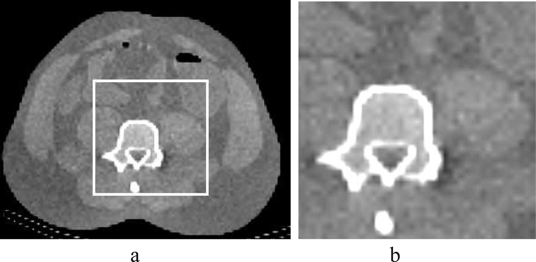
From 720-view data of the pelvis phantom normalized by weighting function W1, we reconstructed by using the FDK algorithm an image on an array of 100×140 pixels of a 0.3-cm size within the middle plane, as shown in Fig. 4. In the inverse-crime study, the reconstruction was used subsequently as the discrete “truth” image from which we generated model data by using ℋ at 720 views uniformly distributed over 2π for a scanning configuration identical to that in real-data studies below. The detector row used consisted of 256 detector bins each of which had a size of 0.1552 cm. The same matrix ℋ was then used in the ASD-WPOCS and EM algorithms in the inverse-crime study.
Figure 4.
(a) Truth discrete image used for generating model data in an inverse-crime study. (b) Image within the ROI enclosed by the white lines in (a), displayed in a zoomed-in view. Display window: [0.1, 0.25] cm−1.
B. Selection of program parameters
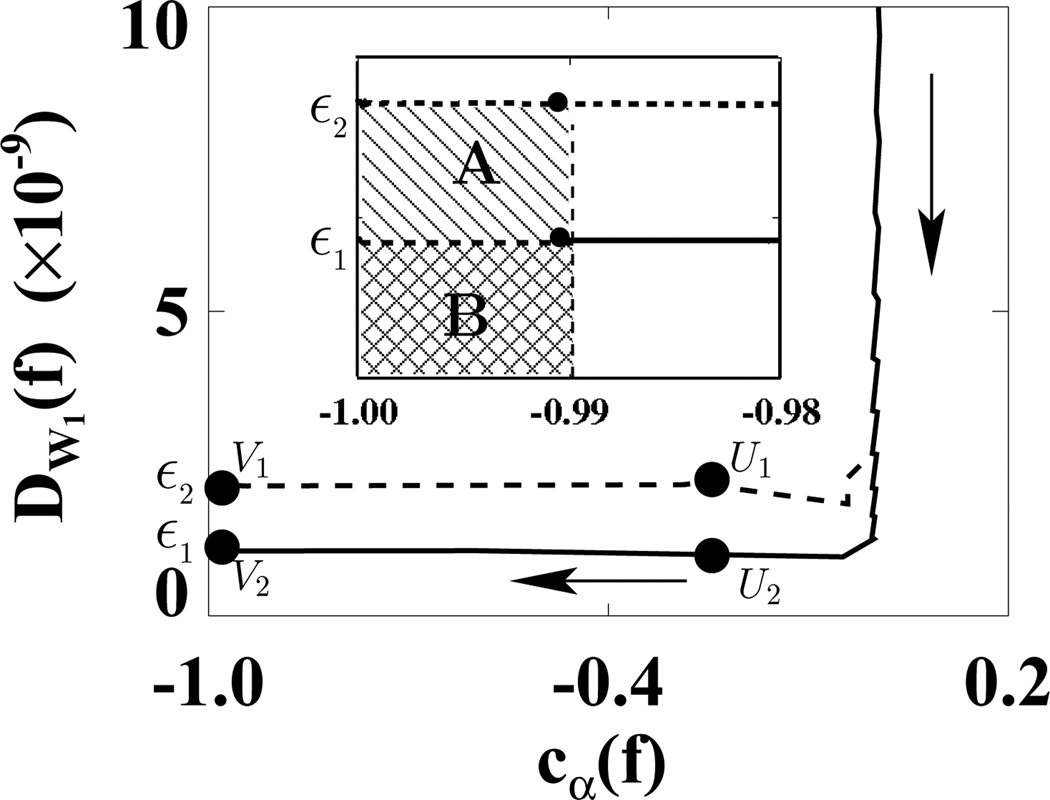
We selected t0 = 239.48, which is the TV of the discrete truth image in Fig. 4, and γ = −0.99, which is sufficiently close to −1. In the inverse-crime study, because the measured data are identical to the model data, the parameter ε should theoretically be set to 0. However, because of limited computer precision, and because of the finite number of iterations used, ε = 0 cannot be reached practically. Moreover, the convergence metric cα(f) becomes undefined when ε = 0 because the data-divergence gradient vector becomes a zero vector [11], and it cannot be employed for monitoring the algorithm convergence at ε = 0. Therefore, for each weighting matrix considered in the study, we selected two descending ε values of ε1 = 1.1 × 10⁻⁹ and ε2 = 2.2 × 10⁻⁹, which are close to zero. The trend of the results from the two values may reveal reconstruction properties near ε = 0. With the data and imaging model described and the parameters selected, the reconstruction program specified by Eq. (3) is completely determined. Images are then reconstructed through solving the program by use of the ASD-WPOCS algorithm.
C. Results of inverse-crime studies
1) Convergence to designed solutions
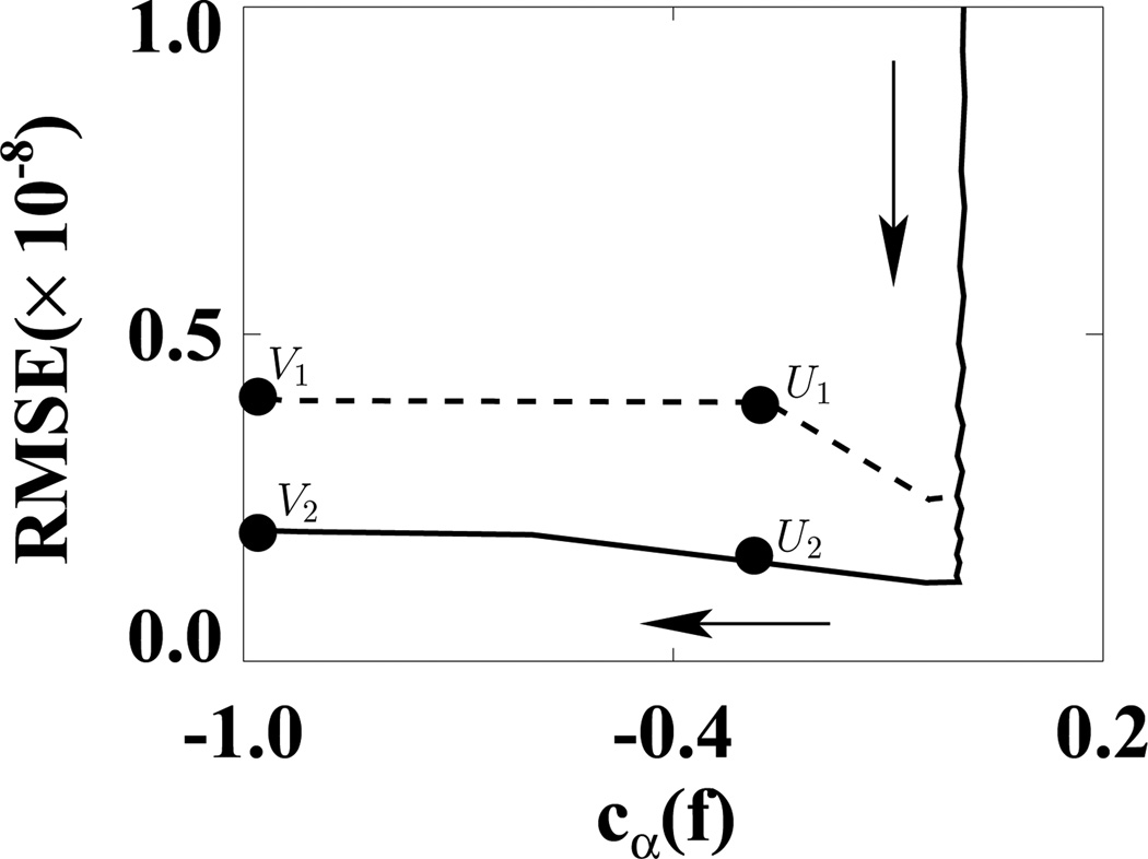
We first used the weighting matrix 𝒲1 in a reconstruction study in which D𝒲1(f) and cα(f) were calculated at each iteration. In Fig. 5, we plotted D𝒲1(f) versus cα(f) for ε1 (solid curve) and ε2 (dashed curve). (We did not use the usual plots of D𝒲1(f) and cα(f) versus iterations because in this way, we can more directly show the algorithm convergence with only one plot.) In the D𝒲1(f)−cα(f) space, the shaded regions indicate two designed solution sets specified by (ε, γ) = (1.1 × 10⁻⁹, −0.99) and (2.2 × 10⁻⁹, −0.99). It can be observed that the ASD-WPOCS algorithm can achieve the designed solution sets numerically. For showing differences between reconstructions and the discrete truth image, we plotted in Fig. 6 their root-mean-square-errors (RMSEs) for ε1 (solid curve) and ε2 (dashed curve). The results also suggest that the ASD-WPOCS algorithm can yield images close to the discrete-truth image in an inverse-crime scenario. As expected, a tighter constraint specified by D𝒲1(f) ≤ ε1 results in a smaller RMSE than does a constraint specified by D𝒲1(f) ≤ ε2.
Figure 5.
Data divergences D𝒲1 as functions of cα(f) calculated for ASD-WPOCS reconstructions with ε1 (solid curve) and ε2 (dashed curve) in inverse-crime studies. Regions A ( ) and B (
 ) in the inserted panel show the designed solution sets, specified by ε1 and ε2 and by γ = −0.99 in a zoomed-in view. The arrow indicates the ascending direction for iteration numbers. The respective numbers of iterations are about 110 at points U1 and U2 and 130 at points V1 and V2.
Figure 6.
RMSEs of ASD-WPOCS reconstructions as functions of cα(f) for ε1 (solid curve) and ε2 (dashed curve) in inverse-crime studies. The arrow indicates the ascending direction for iteration numbers. The respective numbers of iterations are about 110 at points U1 and U2 and 130 at points V1 and V2.
2) Weighting matrices and reconstructions
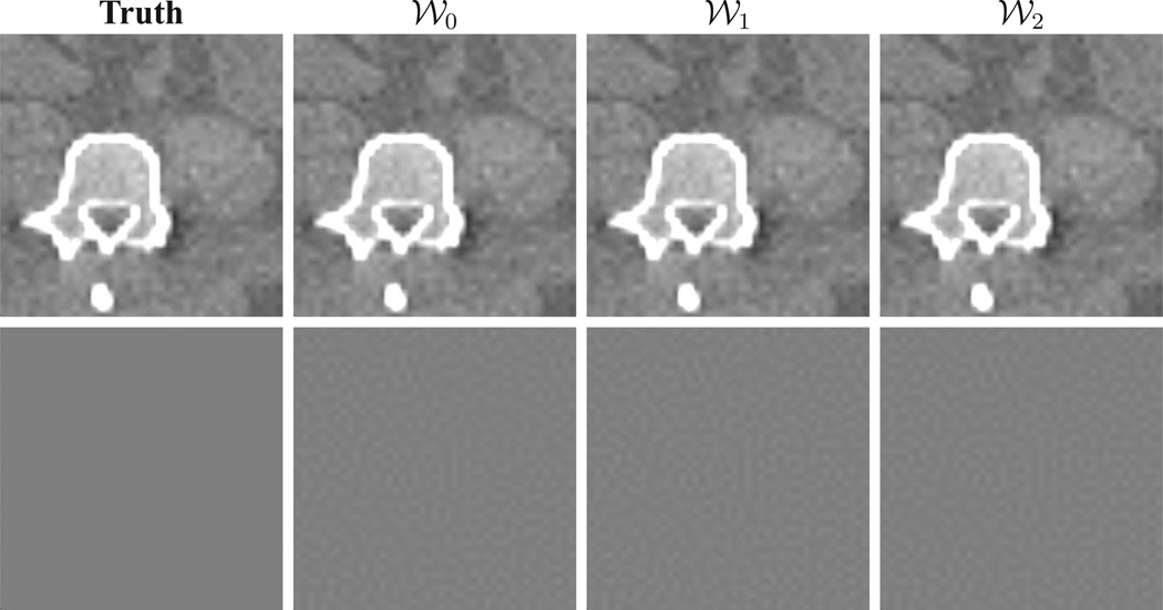
We have also reconstructed images from the same data set by using the ASD-WPOCS algorithm with weighting matrices 𝒲0 and 𝒲2. When identical program parameters were used, results numerically close to those obtained with weighting matrix 𝒲1 were obtained. In row 1 of Fig. 7, we show reconstructions within a region of interest (ROI) in the middle plane with ε1 and weighting matrices 𝒲0, 𝒲1, and 𝒲2, respectively, which are visually identical. For a further comparison, we display the truth ROI image in column 1 of Fig. 7, and the differences between reconstructions and the discrete truth image in row 2 of Fig. 7. The results reveal that an appropriate selection of weighting matrices has, as expected, little impact on image reconstructions in an inverse-crime scenario. However, as will be shown in Sec. VIII below in real-data studies, different weighting matrices can lead to different reconstructions when the data are inconsistent with the D-D imaging model.
Figure 7.
Row 1: Truth ROI image and ROI images reconstructed by use of ASD-WPOCS algorithm with weighting matrices 𝒲0, 𝒲1, and 𝒲2 in inverse-crime studies. Display window: [0.1, 0.25] cm−1. Row 2: Differences between ROI images in row 1 and the truth ROI image. Display window: [−0.00001, 0.00001] cm−1.
We have also carried out an inverse-crime study of reconstruction program 2 and the EM algorithm. Observations can be made similar to those for the inverse-crime study of reconstruction program 1 and the ASD-WPOCS algorithm.
VIII. Real-data studies based on the D-D imaging model
In addition to the inverse-crime verification studies above, we also characterized optimization-based reconstructions by using real data, which are inconsistent with the D-D imaging model. We first performed studies with data acquired from a physical pelvis phantom, followed by studies with data acquired from a patient data were performed.
A. Selection of study parameters
Full-data sets were collected at 720 views uniformly distributed over 2π from the pelvis phantom and patient. From a full-data set, we then extracted sparse-view data sets consisting of projections at 72, 120, 180, and 360 views uniformly distributed over 2π, respectively. From full and sparse-view data, image reconstructions for the pelvis phantom and patient were carried out on arrays of 600×840×175 and 600×840×164, respectively, of prism-shaped voxels defined in Sec. II.
1) Selection of program parameters
For each of the real-data sets and a weighting matrix 𝒲, we determined adaptively parameters specifying the reconstruction programs in Eqs. (3) and (6). For reconstruction program 1, we applied the WPOCS algorithm to the data set to obtain a residual data divergence when successive iterations resulted in little change in D𝒲(f), and select ε around the residual data divergence. Using the selected ε, we ran the ASD-WPOCS algorithm over the data set, calculated reconstruction TV, and selected t0 around the calculated TVs that were flatting out as a function of the iterations. Finally, we chose γ = −0.99. The selected parameters, along with other factors such as image array and voxels, specify reconstruction program 1 and a set of designed solutions. Using the same strategy for reconstruction program 1, we also selected parameters to specify reconstruction program 2.
2) Selection of weighting matrices
The inverse-crime study above suggests that appropriately selected weighting matrices yield numerically virtually identical results. However, in a real-data study, because measured data are inconsistent with the D-D imaging model, different weighting matrices are likely to generate different reconstructions. We conducted a real-data study for determining a weighting matrix to be used in the studies of Secs. VIII-B and VIII-C below.
In the study, images were reconstructed by use of the ASD-WPOCS and EM algorithms with weighting matrices 𝒲0, 𝒲1, and 𝒲2, respectively, from 360-view real data of the pelvis phantom, and we display ASD-WPOCS reconstructions within an ROI in the middle plane in row 1 of Fig. 8. For comparison, we also show their differences relative to the FDK-reference ROI image. It can be observed that the reconstruction with weighting matrix 𝒲1 (column 3) contains minimum artifacts. Artifacts in columns 2 and 4 occurred largely between the region covered by the data of the shaded regions and unshaded region in Fig. 2 b. Similar results were obtained for the EM algorithm [41]. As the weighting matrix 𝒲1 is formed by use of a smooth weighting function W1 in its discrete form, the result is consistent with the observation made for analytic-based reconstructions. Therefore, we used 𝒲1 as the weighting matrix for the real-data studies described below.
B. Results of the pelvis-phantom study
From the full and sparse-view data of the pelvis phantom, we reconstructed images by using the ASD-WPOCS and EM algorithms with weighting matrix 𝒲1. For characterization purposes, FDK images were also reconstructed from the same data sets normalized by weighting function W1.
1) Algorithm-convergence study
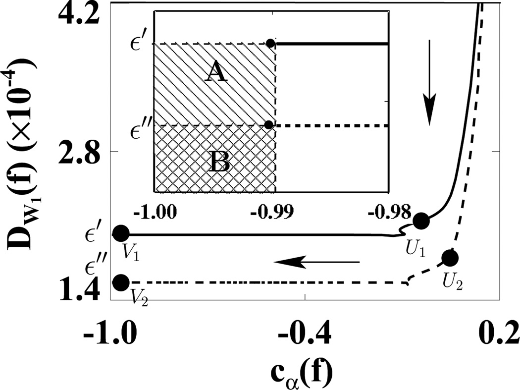
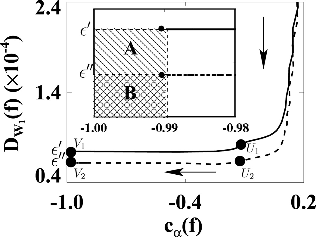
For each of the data sets considered, we have selected program parameters as described in Sec. VIII-A1. We used reconstructions within the middle planes from 72- and 120-view data sets to demonstrate in detail algorithm convergence. Similar results from other data sets can be obtained. For 72- and 120-view data sets we have determined ε′ = 2.0 × 10⁻⁴ and ε″ = 1.6 × 10⁻⁴ and selected γ = −0.99 to specify reconstruction program 1. For each data set, the convergence properties of the ASD-WPOCS algorithm can be evaluated numerically by determining whether it achieves the solution set specified by D𝒲1(f) ≤ ε and cα(f) ≤ γ. The designed solution sets for 72- and 120-view data sets are shown as the shaded regions in a plot of D𝒲1(f) versus cα(f) in Fig. 9. From an ASD-WPOCS reconstruction at each iteration, we calculated D𝒲1(f) and cα(f) and plotted them in Fig. 9 for 72-view (solid) and 120-view (dashed) data sets. The dark circles depicted at the upper-right corners of the shaded regions in the zoomed-in insert indicate the ASD-WPOCS convergence to the respective designed solution sets.
Figure 9.
Data divergences D𝒲1 as functions of cα(f) calculated for ASD-WPOCS reconstructions from 72-view (solid curve) and 120-view (dashed curve) pelvis-phantom data. Regions A ( ) and B (
 ) in the inserted panel show the designed solution sets determined for 72- and 120-view studies in a zoomed-in view. The arrow indicates the ascending direction for iteration numbers. The respective numbers of iterations are about 90 at points U1 and U2 and 300 at points V1 and V2.
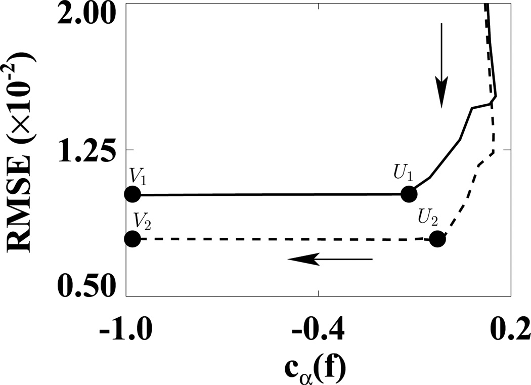
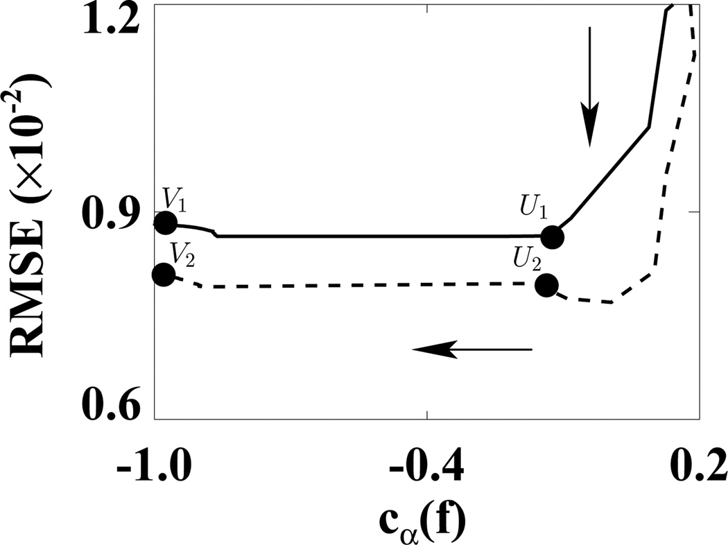
In Fig. 10, we show RMSEs of the reconstructions relative to the FDK-reference reconstruction as a function of cα(f). It can be observed that RMSEs flattened out around points U1 and U2 for the 72- and 120-view cases before approaching the designed solutions at points V1 and V2 constrained by cα(f) < −0.99. For the 72- and 120-view cases, the respective numbers of iterations are about 90 at points U1 and U2 and 300 at convergent points V1 and V2. Images appear to be of little visual difference at iterations between U1 and V1 for the 72-view case and between U2 and V2 for the 120-view case. The results shown below were obtained with iterations around V1 and V2 for 72- and 120-view cases.
Figure 10.
RMSEs as functions of cα(f) calculated from ASD-WPOCS reconstructions relative to the FDK-reference image for 72-view (solid curve) and 120-view (dashed curve) data sets of the pelvis phantom. The arrow indicates the ascending direction for iteration numbers. The respective numbers of iterations are about 90 at points U1 and U2 and 300 at points V1 and V2.
2) Reconstruction visualization
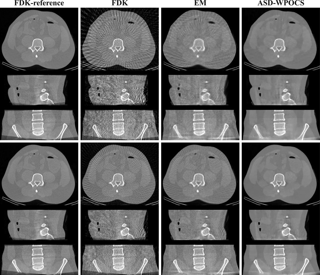
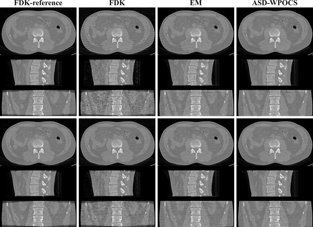
In Fig. 11, we show 3D images within transverse, sagittal, and coronal slices using a wide display window, images reconstructed by use of the FDK, EM, and ASD-WPOCS algorithms from the 72-view (rows 1–3) and 120-view (rows 4–6) data sets. The corresponding FDK-reference images are displayed also in column 1 of Fig. 11 for visual comparison. The images are redisplayed with a narrow display window in Fig. 12. As expected, streak artifacts can be observed in FDK reconstructions from 72- and 120-view data sets. When the images are showed with a narrow display window in Fig. 12, some streak artifacts are revealed also in EM reconstructions. On the other hand, the ASD-WPOCS reconstructions appear to be relatively free of visual artifacts, while preserving low-contrast details observed in the FDK-reference images.
Figure 11.
Images reconstructed from 72-view (rows 1–3) and 120-view (rows 4–6) pelvis-phantom-data sets by use of the FDK, EM, and ASD-WPOCS algorithms, within a transverse slice at z = 0 cm (rows 1 and 4), coronal slice at x = 1.0 cm (rows 2 and 5), and sagittal slice at y = −1.0 cm (rows 3 and 6). Display window: [0, 0.35] cm−1.
Figure 12.
Images identical to those in Fig. 11 but displayed with a narrow window of [0.1, 0.25] cm−1.
3) Reconstruction characterization
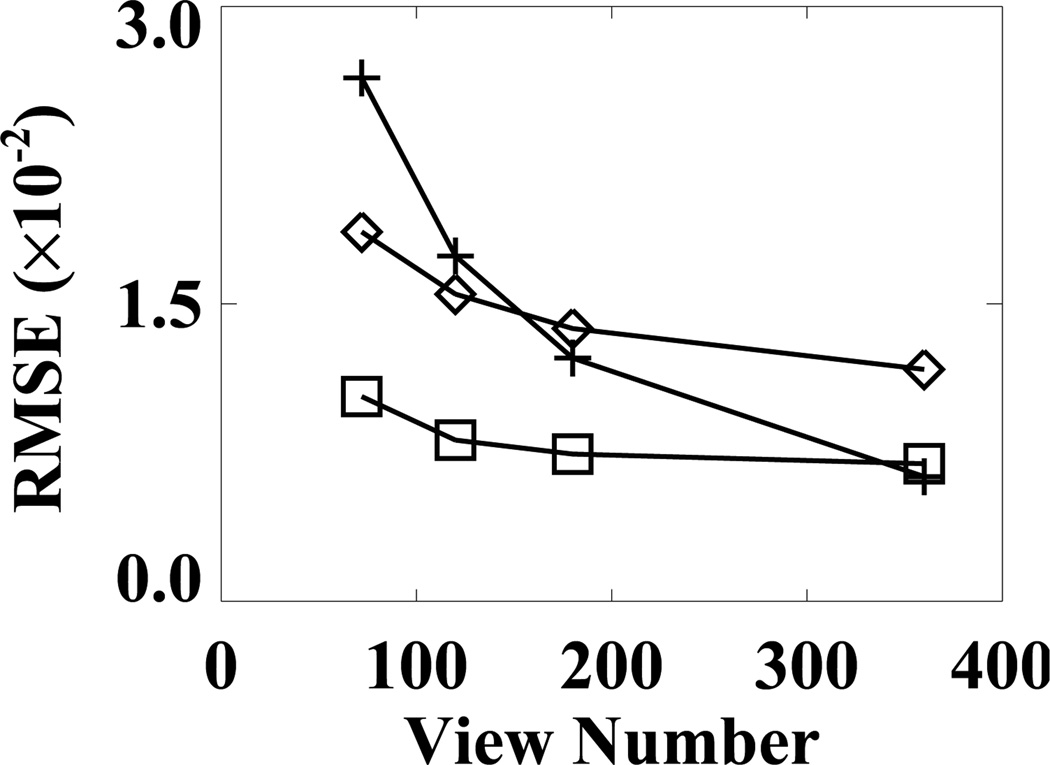
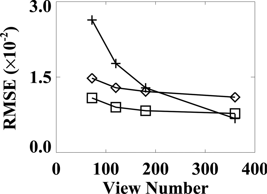
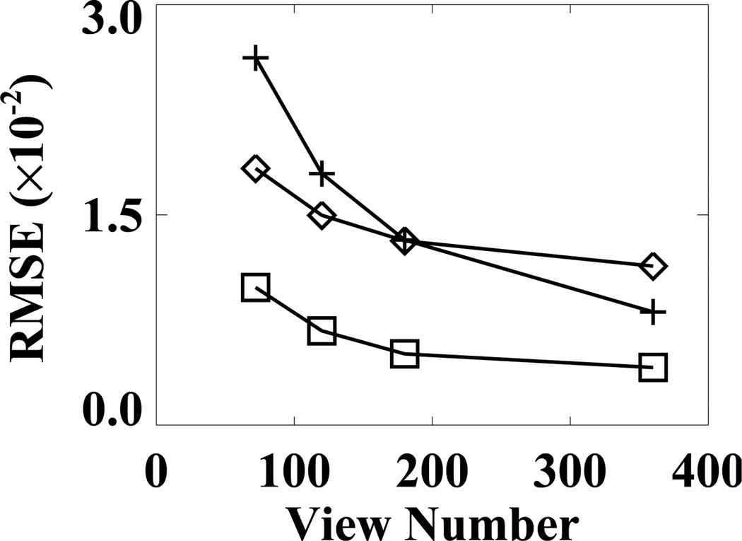
We characterized the properties of the FDK, EM, and ASD-WPOCS reconstructions from sparse-view data by calculating their respective RMSEs relative to the FDK-reference reconstruction, and plotted them as functions of view numbers in Fig. 13. The ASD-WPOCS reconstructions appear to yield RMSEs lower than those of the other reconstructions, except that it is comparable to the FDK RMSE for the 360-view case. As explained in Sec. IX below, this is because the FDK-reference image used is in favor of the FDK RMSE calculation for large view numbers. It can also be observed that the differences among the algorithms decrease as the view number increases.
Figure 13.
RMSEs of FDK (+), EM (⋄), and ASD-WPOCS (□) reconstructions relative to the FDK-reference image as functions of the view number for pelvis-phantom data.
From the reconstructions, we also calculated additional numeric metrics such as the universal quality index (UQI) [42] and mutual information (MI) [43] with respect to the FDK-reference image and observed that these metrics yielded information about reconstructions similar to the RMSE results above.
4) Computation of attenuation factors
An application of CT images in SPECT/CT imaging is to estimating attenuation factors for use in correction for attenuation artifacts in SPECT. We calculated attenuation factors from reconstructed CT images and compared them to that obtained from the FDK-reference image.
The attenuation factor in a continuous form is defined as
| (12) |
where f(r) denotes the attenuation map at a spatial point r, which is an image reconstructed from CBCT data, and the unit vector θ̂ denotes the direction of a gamma ray in SPECT imaging. Without loss of generality, we consider a parallel-beam collimation in SPECT imaging. Therefore, the integration in Eq. (12) can be carried out within a transverse plane. We considered the calculation of an attenuation factor for the middle plane, while realizing that such a calculation can readily be carried out for non-middle planes. The attenuation factor within the middle plane is then discretized on a 300×420×720 array in which the first two dimensions are for r, with a pixel size of 0.1 cm, and the third dimension is for the angle with an interval of 0.5°.
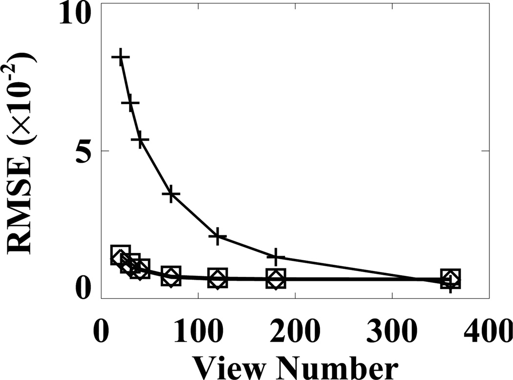
For characterization of CT-image reconstructions in terms of attenuation-factor estimation, we performed reconstructions by using the FDK, EM, and ASD-WPOCS algorithms from data sets containing view numbers ranging from 20 to 40 in addition to the reconstructions from the data sets previous extracted. Using these reconstructions, we estimated the attenuation factors, and then calculated their RMSEs relative to that obtained from the FDK-reference image, and display them in Fig. 14 as functions of a view number. The result suggests that, if the task is to estimate an attenuation factor, the EM and ASD-WPOCS algorithms can yield numerically comparable attenuation factors and that the attenuation factor is a slowly varying function of the view number used for reconstruction of the attenuation map. When an integration of the attenuation factor is carried out over the angle, one obtains the so-called Chang’s factor [44], which has been used for obtaining an approximate attenuation correction for FBP reconstruction of SPECT images. We also computed the Chang’s factors for data sets considered and compared them with that obtained with the FDK-reference image. Again, results and observations similar to those for the attenuation-factor estimation were obtained.
Figure 14.
RMSEs of attenuation factors computed from FDK (+), EM (⋄), and ASD-WPOCS (□) reconstructions, respectively, relative to the attenuation factor computed from the FDK-reference image, as functions of the view number.
C. Results of the patient study
From the 720-view data set acquired from a patient, we extracted sparse-view data containing 72, 120, 180, and 360 views uniformly distributed over 2π, from which we reconstructed images by using the ASD-WPOCS and EM algorithms with weighting matrix 𝒲1. Again, for the purpose of characterization, FDK images were also reconstructed from the data sets normalized by weighting function W1.
1) Algorithm-convergence study
For each of the data sets, we selected program parameters as described in Sec. VIII-A1. Without loss of generality, we used reconstructions within the middle planes only from 120- and 180-view data sets to demonstrate algorithm convergence. For 120- and 180-view data sets, we first determined ε′ = 7.4 × 10⁻⁵ and ε″ = 6.2 × 10⁻⁵ and selected γ = −0.99 to specify reconstruction program 1. For each data set, the convergence property of the ASD-WPOCS algorithm can be evaluated numerically as to whether it achieves the solution set specified by D𝒲1 (f) ≤ ε and cα(f) ≤ γ. The designed solution sets for 120- and 180-view data sets are shown as shaded regions in a plot of D𝒲1(f) versus cα(f), as displayed in Fig. 15. From an ASD-WPOCS reconstruction at each iteration, we then calculated D𝒲1 (f) and cα(f) and plotted them in Fig. 15 for 120-view (solid) and 180-view (dashed) data sets. Again, the dark circles depicted at the upper-right corners of the shaded regions in the zoomed-in insert suggest the ASD-WPOCS convergence to the respective designed solution sets.
Figure 15.
Data divergences D𝒲1 as functions of cα(f) calculated for ASD-WPOCS reconstructions from 120-view (solid curve) and 180-view (dashed curve) patient data. Regions A ( ) and B (
 ) in the inserted panel show the designed solution sets determined for 120- and 180-view studies in a zoomed-in view. The arrow indicates the ascending direction for iteration numbers. The respective numbers of iterations are about 60 at points U1 and U2 and 300 at points V1 and V2.
In Fig. 16, we also show RMSEs of the reconstructions relative to the FDK-reference reconstruction as a function of cα(f). It can again be observed that RMSEs flattened out around points U1 and U2 for the 120- and 180-view cases before approaching the designed solutions at points V1 and V2 constrained by cα(f) < −0.99. For the two cases, the respective numbers of iterations are about 60 at points U1 and U2 and 300 at convergent points V1 and V2. Images appear to be of little visual difference at iterations between U1 and V1 for the 120-view case and between U2 and V2 for the 180-view case. The results shown below were obtained with iterations around V1 and V2 for 120- and 180-view cases.
Figure 16.
RMSEs as functions of cα(f) calculated from ASD-WPOCS reconstructions relative to the FDK-reference image for 120-view (solid curve) and 180-view (dashed curve) data sets of the patient. The arrow indicates the ascending direction for iteration numbers. The respective numbers of iterations are about 60 at points U1 and U2 and 300 at points V1 and V2.
2) Reconstruction visualization
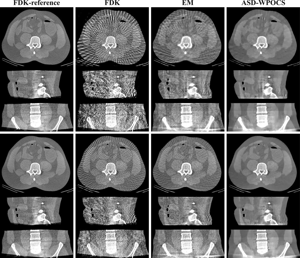
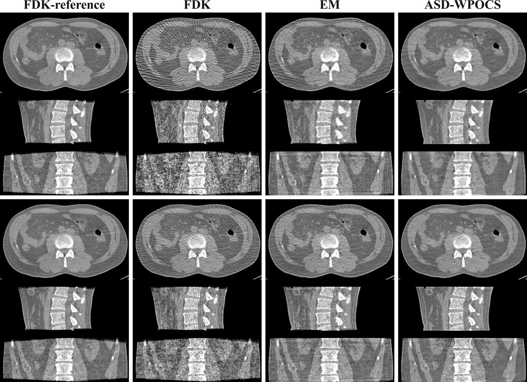
In Fig. 17, we show 3D images within transverse, sagittal, and coronal slices with a wide display window, reconstructed by use of the FDK, EM, and ASD-WPOCS algorithms from the 120-view (rows 1–3) and 180-view (rows 4–6) data sets. The corresponding FDK-reference images are displayed also in column 1 of Fig. 17 for visual comparison. The images are re-displayed with a narrow window in Fig. 18 for revealing additional details. Again, some streak artifacts can be observed in FDK reconstructions from 120- and 180-view data sets. When shown with a narrow display window, mild streak artifacts also appear in the EM reconstructions. In contrast, the ASD-WPOCS reconstructions are relatively free of visual artifacts and reveal the low-contrast details observed in FDK-reference images.
Figure 17.
Images reconstructed from 120-view (rows 1–3) and 180-view (rows 4–6) patient-data sets by use of the FDK, EM, and ASD-WPOCS algorithms, within a transverse slice at z = 0 cm (rows 1 and 4), coronal slice at x = 1.0 cm (rows 2 and 5), and sagittal slice at y = −1.0 cm (rows 3 and 6). Display window: [0, 0.35] cm−1.
Figure 18.
Images identical to those in Fig. 17 but displayed with a narrow window of [0.1, 0.25] cm−1.
3) Reconstruction characterization
We also characterized the properties of the FDK, EM, and ASD-WPOCS reconstructions from sparse-view data by calculating their respective RMSEs relative to the FDK-reference reconstruction, and we plotted them as functions of view numbers in Fig. 19. Results and observations similar to those acquired in the phantom study above can be obtained for the patient study. From the reconstructions, we also calculated other numeric metrics such as the UQI and MI with respect to the FDK-reference image and observed that these metrics yield information about reconstructions similar to the RMSE results.
Figure 19.
RMSEs of FDK (+), EM (⋄), and ASD-WPOCS (□) reconstructions relative to the FDK-reference image as functions of the view number for patient data.
IX. Discussion
The work investigates analytic- and optimization-based image reconstructions from data, and particularly from sparse-view data, acquired in offset-detector CBCT. We discussed analytic- and optimization-based algorithms in parallel for the purpose of clarifying relationships between C-C and D-D imaging models and between analytic- and optimization-based algorithms [45]. Although there can be conceptual cross over between the C-C and D-D imaging models, they possess distinctly different properties that demand different approaches to analyzing and inverting them. An analytic-based algorithm in its discrete form in general is not the solution to the D-D imaging model. A contrast was made carefully on the implications of data redundancy in a C-C imaging model and linearity in a D-D imaging model. Although the C-C and D-D image models are distinctly different, observations of the redundancy property of the C-C imaging model can provide insights into, e.g., the design of a weighting matrix in a D-D imaging model for facilitating reconstructions with minimized artifacts in the presence of data inconsistencies. It should be pointed out that weighting matrices exploiting the linearity of a D-D model may also be designed for yielding reconstructions with desired properties in CBCT.
We have also conducted inverse-crime studies in the work for verifying that the algorithms discussed can indeed achieve the designed solution sets. Additional studies were carried out for characterizing algorithm properties in studies using real data that are inconsistent with the imaging model upon which algorithm development is based. In terms of metrics used in the studies, even though the ASD-WPOCS algorithm seems to perform better than other algorithms considered, the studies are not intended to promote the ASD-WPOCS algorithm’s clinical utility, which remains to be evaluated in specific clinical applications. However, we believe that, if an algorithm performs worse than other algorithms in the study, it is unlikely that the algorithm can perform better than other algorithms in practical, clinical studies.
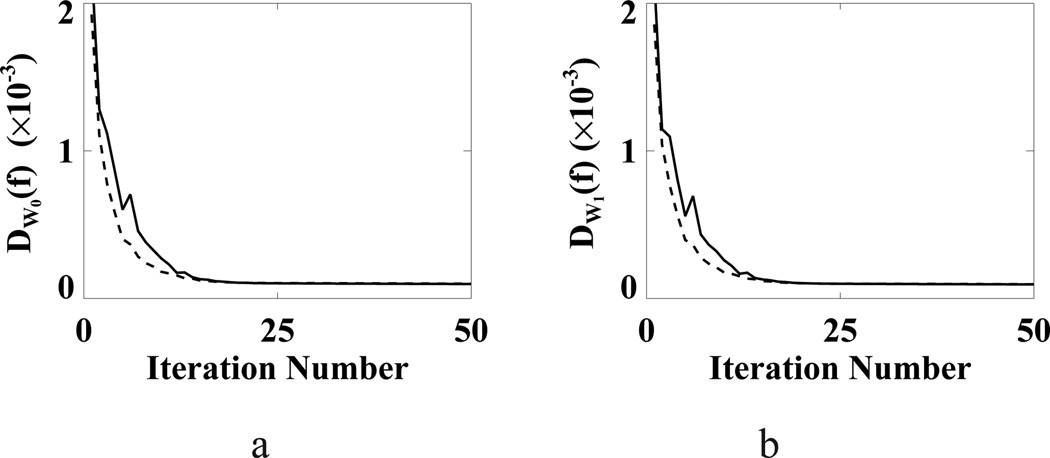
The results above show that the WPOCS algorithm can lower the weighted Euclidean data divergence D𝒲(f), whereas it is unclear whether the WPOCS algorithm can minimize D𝒲(f) in the presence of data inconsistency. We point out that an appropriately selected weighting matrix may potentially enhance the effectiveness of the WPOCS in reducing D𝒲(f), which is demonstrated by the following study: Using weighting matrices 𝒲0 and 𝒲1, we can obtain the POCS algorithm and a WPOCS algorithm from Eq. (7), and also form data divergences D𝒲0(f) and D𝒲1(f). Applying the POCS and WPOCS algorithms to the pelvis-phantom data, we reconstructed images from which we then computed D𝒲0(f) and D𝒲1(f) and show them in Fig. 20. The result suggests that the WPOCS with 𝒲1 lowers D𝒲0(f) and D𝒲1 (f) faster than does the POCS. Therefore, it may be worthy of investigating the design of the weighting matrices for enhancing the WPOCS efficiency.
Figure 20.
(a) D𝒲0 and (b) D𝒲1 as functions of iteration numbers obtained by use of WPOCS with weighting matrices 𝒲0 (solid curve) and 𝒲1 (dashed curve) from pelvis-phantom data.
In the work, the WPOCS algorithm was used for lowering the weighted Euclidean data divergence. When further calculation of the divergence becomes necessary for reducing cα(f), we used algorithms such as gradient descent to replace the WPOCS. Other algorithms such as simultaneous algebraic reconstruction technique (SART) algorithm [46]–[48] can readily be modified to accommodate an offset-detector configuration. The computation time of the ASD-WPOCS algorithm is related with several factors, including iteration number, algorithm implementation, and computation hardware. The computation speed of the algorithms considered can be enhanced substantially through streamlining/parallelizing its implementation and/or by exploiting the available, or rapidly available, high performance computational hardware.
The algorithm properties depend upon a number of parameters, including data amount and characterization methods/metrics. For example, significant artifacts can be observed in images reconstructed from data sets containing 20–40 projections of the pelvis phantom and patient. However, as Fig. 14 shows, for the task of estimating attenuation factors, the EM and ASD-WPOCS results from data sets of 20–40 projections are comparable to that obtained from data sets containing 60 or more views, in terms of a RMSE-metric assessment. Therefore, if the estimation of attenuation factors is of concern, data sets of 20–40 views could be sufficient, even though visible artifacts can be observed in CT-image reconstructions.
The RMSE results above were obtained with FDK-reference images. Clearly, it may change quantitatively when different reference images are used. In column 2 of Fig. 3, we display images reconstructed by use of the ASD-WPOCS algorithm from the respective full-data sets of the pelvis phantom and patient. These images, which we refer to as the ASD-WPOCS-reference images, can also be used for replacing the FDK-reference images in RMSE calculations, thus yielding RMSE results different from those obtained with the FDK-reference image. In Fig. 21, we show the RMSE results obtained with an ASD-WPOCS-reference image obtained with 𝒲1 for the pelvis phantom. Its comparison with the corresponding results in Fig. 13 obtained with the FDK-reference image indicates clear differences in RMSE results, and it can be observed that the ASD-WPOCS performs considerably better than FDK and EM even at large number (e.g., 360) of views in this case. Similar results were obtained for reconstructions from patient data.
Figure 21.
RMSEs of FDK (+), EM (⋄), and ASD-WPOCS (□) reconstructions relative to the ASD-WPOCS-reference image as functions of the view number for pelvis-phantom data.
In this work, we considered FDK, EM, and ASD-WPOCS algorithms for a reconstruction problem in offset-detector CBCT. Although additional algorithms may be developed for solving this problem, they are beyond the scope of the current work. The inclusion of the FDK and EM reconstructions from sparse-view data was for benchmarking the corresponding ASD-WPOCS reconstructions in the characterization studies. They are not intended to justify the practical utility of the ASD-WPOCS algorithm, which still remains to be evaluated in real clinical applications. Also, we have studied in the work image reconstructions from data containing different numbers of projections, with comparable signal-to-noise ratios (SNRs, i.e. radiation dose levels). However, it is of high practical interest to investigate how a trade-off between view numbers and data SNR would impact the reconstruction properties [49]–[51].
X. Conclusion
In the work, we investigated and demonstrated image reconstructions by using the FDK, EM, and ASD-WPOCS algorithms in offset-detector CBCT. Quantitative studies were carried out for verifying and characterizing the reconstruction properties of the algorithms. From the study results, it appears that the ASD-WPOCS algorithm performs better than the FDK and EM algorithms for conditions of practical interest in terms of the metrics considered. The results of the sparse-view study can have a potentially significant implication for dose reduction in CBCT imaging in SPECT/CBCT applications. Furthermore, it can readily be extended to reducing the radiation dose of CBCT imaging in image-guided surgery and radiation therapy, and in other emerging CBCT applications in which an offset-detector configuration is used.
Acknowledgments
The authors would like to thank Dr. Dan Xia and Professor Chien-Min Kao for helpful discussions. This work was supported in part by the National Institutes of Health (NIH) under Grants CA120540 and EB000225. The work of X. Han was supported in part by the Department of Defense (DoD) Predoctoral training Grants PC094510. Some computation in the work was performed on a cluster partially funded by the University of Chicago for Comprehensive Cancer Center.
References
- 1.Hasegawa BH, Gingold EL, Reilly SM, Liew SC, Cann CE. Description of a simultaneous emission-transmission CT system. Proc. SPIE. 1990;vol. 1231:50. [Google Scholar]
- 2.Lang TF, Hasegawa BH, Liew SC, Brown KJ, Blankespoor SC, Reilly SM, Gingold EL, Cann CE. Description of a prototype emission transmission computed tomography imaging. J. Nucl. Med. 1992;vol. 33:1881–1887. [PubMed] [Google Scholar]
- 3.Bocher M, Balan A, Krausz Y, Shrem Y, Lonn A, Wilk M, Chisin R. Gamma camera-mounted anatomical X-ray tomography: technology, system characteristics and first images. Eur. J. Nucl. Med. Mol. Imaging. 2000;vol. 27:619–627. doi: 10.1007/s002590050555. [DOI] [PubMed] [Google Scholar]
- 4.Patton JA, Delbeke D, Sandier MP. Image fusion using an integrated, dual-head coincidence camera with X-ray tube-based attenuation maps. J. Nucl. Med. 2000;vol. 41:1364–1368. [PubMed] [Google Scholar]
- 5.Hasegawa B, Wong K, Iwata K, Barber W, Hwang A, Sakdinawat A, Ramaswamy M, Price D, Hawkins R. Dual-modality imaging of cancer with SPECT/CT. Techno. Cancer Res. Treat. 2002;vol. 1:449–458. doi: 10.1177/153303460200100605. [DOI] [PubMed] [Google Scholar]
- 6.Sowards-Emmerd D, Vesel J, Shao L, Timmer J, Bertram M, Ye J, Hines H. Seminars in Nuclear Medicine. Elsevier; 2009. Flat Panel X-ray Detector Based Volume Imaging SPECT/CT. [Google Scholar]
- 7.Sowards-Emmerd D, Balakrishnan K, Wiener J, Shao L, Ye J. CBCT-subsystem performance of the multi-modality Brightview XCT system; Nucl. Sci. Symp. Conf. Rec. (NSS/MIC); 2009. pp. 3053–3058. IEEE. [Google Scholar]
- 8.Chang W, Loncaric S, Huang G, Sanpitak P. Asymmetric fan transmission CT on SPECT systems. Phys. Med. Biol. 1995;vol. 40:913–928. doi: 10.1088/0031-9155/40/5/013. [DOI] [PubMed] [Google Scholar]
- 9.Cho PS, Johnson RH, Griffint TW. Cone-beam CT for radiotherapy applications. Phys. Med. Biol. 1995;vol. 40:1863–1883. doi: 10.1088/0031-9155/40/11/007. [DOI] [PubMed] [Google Scholar]
- 10.Sidky EY, Kao K-M, Pan X. Accurate image reconstruction from few-views and limited-angle data in divergent-beam CT. J. X-Ray Sci. and Technol. 2006;vol. 14:119–139. [Google Scholar]
- 11.Sidky EY, Pan X. Image reconstruction in circular cone-beam computed tomography by constrained, total-variation minimization. Phys. Med. Biol. 2008;vol. 53:4777–4807. doi: 10.1088/0031-9155/53/17/021. [DOI] [PMC free article] [PubMed] [Google Scholar]
- 12.Bian J, Siewerdsen JH, Han X, Sidky EY, Prince JL, Pelizzari CA, Pan X. Evaluation of sparse-view reconstruction from flat-panel-detector cone-beam CT. Phys. Med. Biol. 2010;vol. 55:6575–6599. doi: 10.1088/0031-9155/55/22/001. [DOI] [PMC free article] [PubMed] [Google Scholar]
- 13.Han X, Bian J, Eaker DR, Kline TL, Sidky EY, Ritman EL, Pan X. Algorithm-enabled low-dose micro-CT imaging. IEEE Trans. Med. Imag. 2011;vol. 30:606–620. doi: 10.1109/TMI.2010.2089695. [DOI] [PMC free article] [PubMed] [Google Scholar]
- 14.Li M, Yang H, Kudo H. An accurate iterative reconstruction algorithm for sparse objects: application to 3D blood vessel reconstruction from a limited number of projections. Phys. Med. Biol. 2002;vol. 47:2599–2609. doi: 10.1088/0031-9155/47/15/303. [DOI] [PubMed] [Google Scholar]
- 15.Choi K, Wang J, Zhu L, Suh T-S, Boyd S, Xing L. Compressed sensing based cone-beam computed tomography reconstruction with a first-order method. Med. Phys. 2010;vol. 37:5113–5125. doi: 10.1118/1.3481510. [DOI] [PMC free article] [PubMed] [Google Scholar]
- 16.Ritschl L, Bergner F, Fleischmann C, Kachelrieß M. Improved total variation-based CT image reconstruction applied to clinical data. Phys. Med. Biol. 2011;vol. 56:1545–1561. doi: 10.1088/0031-9155/56/6/003. [DOI] [PubMed] [Google Scholar]
- 17.Ramirez-Giraldo JC, Trzasko J, Leng S, Yu L, Manduca A, McCollough CH. Nonconvex prior image constrained compressed sensing (NCPICCS): Theory and simulations on perfusion CT. Med. Phys. 2011;vol. 38:2157–2167. doi: 10.1118/1.3560878. [DOI] [PMC free article] [PubMed] [Google Scholar]
- 18.Defrise M, Vanhove C, Liu X. An algorithm for total variation regularization in high-dimensional linear problems. Inverse Probl. 2011;vol. 27:065002. [Google Scholar]
- 19.Rashed EA, Kudo H. Statistical image reconstruction from limited projection data with intensity priors. Phys. Med. Biol. 2012;vol. 57:2039–2061. doi: 10.1088/0031-9155/57/7/2039. [DOI] [PubMed] [Google Scholar]
- 20.Lauzier PT, Tang J, Chen G-H. Prior image constrained compressed sensing: Implementation and performance evaluation. Med. Phys. 2012;vol. 39:66–80. doi: 10.1118/1.3666946. [DOI] [PMC free article] [PubMed] [Google Scholar]
- 21. [Online]. Available: http://www.cirsinc.com/products/all/38/virtuallyhuman-male-pelvis-phantom/
- 22.Colton DL, Kress R. Inverse acoustic and electromagnetic scattering theory. Berlin: Springer-Verlag; 1992. [Google Scholar]
- 23.Wirgin A. The inverse crime. arXiv:math-ph/0401050v1. 2004 [Google Scholar]
- 24.Kaipioa J, Somersalob E. Statistical inverse problems: discretization, model reduction and inverse crimes. J. Comput. Appl. Math. 2007;vol. 198:493–504. [Google Scholar]
- 25.Feldkamp LA, Davis LC, Kress JW. Practical cone-beam algorithm. J. Opt. Soc. Am. A. 1984;vol. 1:612–619. [Google Scholar]
- 26.Tuy HK. An inversion formula for cone-beam reconstruction. SIAM J. Appl. Math. 1983;vol. 43:546–552. [Google Scholar]
- 27.Katsevich A. Theoretically exact filtered backprojection-type inversion algorithm for spiral CT. SIAM J. Appl. Math. 2002;vol. 62:2012–2026. [Google Scholar]
- 28.Zou Y, Pan X. Exact image reconstruction on PI-lines from minimum data in helical cone-beam CT. Phys. Med. Biol. 2004;vol. 49:941–959. doi: 10.1088/0031-9155/49/6/006. [DOI] [PubMed] [Google Scholar]
- 29.Pack JD, Noo F, Clackdoyle R. Cone-beam reconstruction using the backprojection of locally filtered projections. IEEE Trans. Med. Imag. 2005;vol. 24:70–85. doi: 10.1109/tmi.2004.837794. [DOI] [PubMed] [Google Scholar]
- 30.Zou Y, Pan X, Sidky EY. Theory and algorithms for image reconstruction on chords and within region of interests. J. Opt. Soc. Am. A. 2005;vol. 22:2372–2384. doi: 10.1364/josaa.22.002372. [DOI] [PubMed] [Google Scholar]
- 31.Pan X, Yu L. Image reconstruction with shift-variant filtration and its implication for noise and resolution properties in fan-beam computed tomography. Med. Phys. 2003;vol. 30:590–600. doi: 10.1118/1.1556608. [DOI] [PubMed] [Google Scholar]
- 32.Xia D, Yu L, Sidky EY, Zou Y, Zuo N, Pan X. Noise properties of chord-image reconstruction. IEEE Trans. Med. Imag. 2007;vol. 26:1328–1344. doi: 10.1109/TMI.2007.898567. [DOI] [PubMed] [Google Scholar]
- 33.Parker DL. Optimal short scan convolution reconstruction for fan beam CT. Med. Phys. 1982;vol. 9:254–257. doi: 10.1118/1.595078. [DOI] [PubMed] [Google Scholar]
- 34.Barrett HH, Myers KJ. Foundations of Image Science. John Wiley Sons, Inc.; 2003. [Google Scholar]
- 35.Dempster AP, Laird NM, Rubin DB. Maximum likelihood from incomplete data via the EM algorithm. J. R. Stat. Soc. Series B Stat. Methodol. 1977;vol. 39:1–38. [Google Scholar]
- 36.Shepp LA, Vardi Y. Maximum likelihood reconstruction for emission tomography. IEEE Trans. Med. Imag. 1982;vol. 1:113–122. doi: 10.1109/TMI.1982.4307558. [DOI] [PubMed] [Google Scholar]
- 37.Han X, Bian J, Ritman EL, Sidky EY, Pan X. Optimization-based reconstruction of sparse images from few-view projections. Phys. Med. Biol. 2012 doi: 10.1088/0031-9155/57/16/5245. Accepted. [DOI] [PMC free article] [PubMed] [Google Scholar]
- 38.Gordon R, Bender R, Herman GT. Algebraic reconstruction techniques (ART) for three-dimensional electron microscopy and X-ray photography. J. Theor. Biol. 1970;vol. 29:471–481. doi: 10.1016/0022-5193(70)90109-8. [DOI] [PubMed] [Google Scholar]
- 39.Youla DC, Webb H. Image restoratoin by the method of convex projections: Part 1 – theory. IEEE Trans. Med. Imag. 1982;vol. 1:81–94. doi: 10.1109/TMI.1982.4307555. [DOI] [PubMed] [Google Scholar]
- 40.Combettes PL. The foundations of set theoretic estimation. Proc. IEEE. 1993;vol. 81:182–208. [Google Scholar]
- 41.Hansis E, Bredno J, Sowards-Emmerd D, Shao L. Iterative reconstruction for circular cone-beam CT with an offset flat-panel detector; Nucl. Sci. Symp. Conf. Rec. (NSS/MIC); 2010. pp. 2228–2231. IEEE. [Google Scholar]
- 42.Wang Z, Bovik A. A universal image quality index. IEEE Signal Process. Lett. 2002;vol. 9:81–84. [Google Scholar]
- 43.Pluim JPW, Maintz JBA, Viergever MA. Mutual-information-based registration of medical images: a survey. IEEE Trans. Med. Imag. 2003;vol. 22:986–1004. doi: 10.1109/TMI.2003.815867. [DOI] [PubMed] [Google Scholar]
- 44.Chang L-T. A method for attenuation correction in radionuclide computed tomography. IEEE Trans. Nucl. Sci. 1978;vol. 25:638–643. [Google Scholar]
- 45.Pan X, Sidky EY, Vannier M. Why do commercial CT scanners still employ traditional, filtered back-projection for image reconstruction? Inverse Probl. 2009;vol. 25:123009. doi: 10.1088/0266-5611/25/12/123009. [DOI] [PMC free article] [PubMed] [Google Scholar]
- 46.Andersen AH, Kak AC. Simultaneous algebraic reconstruction technique (SART): a superior implementation of the ART algorithm. Ultrason. Imaging. 1984;vol. 6:81–94. doi: 10.1177/016173468400600107. [DOI] [PubMed] [Google Scholar]
- 47.Jiang M, Wang G. Convergence studies on iterative algorithms for image reconstruction. IEEE Trans. Med. Imag. 2003;vol. 22:569–579. doi: 10.1109/TMI.2003.812253. [DOI] [PubMed] [Google Scholar]
- 48.Wang J, Zheng Y. On the convergence of generalized simultaneous iterative reconstruction algorithms. IEEE Trans. Image Process. 2007;vol. 16:1–6. doi: 10.1109/tip.2006.887725. [DOI] [PubMed] [Google Scholar]
- 49.Tang J, Nett BE, Chen G-H. Performance comparison between total variation (TV)-based compressed sensing and statistical iterative reconstruction algorithms. Phys. Med. Biol. 2009;vol. 54:5781–5804. doi: 10.1088/0031-9155/54/19/008. [DOI] [PMC free article] [PubMed] [Google Scholar]
- 50.Han X, Pearson E, Bian J, Cho S, Sidky EY, Pelizzari CA, Pan X. Preliminary investigation of dose allocation in low-dose cone-beam CT; Nucl. Sci. Symp. Conf. Rec. (NSS/MIC); 2010. pp. 2051–2054. IEEE. [Google Scholar]
- 51.Yan H, Cervino L, Jia X, Jiang SB. A comprehensive study on the relationship between the image quality and imaging dose in low-dose cone beam CT. Phys. Med. Biol. 2012;vol. 57:2063–2080. doi: 10.1088/0031-9155/57/7/2063. [DOI] [PMC free article] [PubMed] [Google Scholar]


