Investigation of the freely available easy-to-use software ‘EZR' for medical statistics

Abstract

Although there are many commercially available statistical software packages, only a few implement a competing risk analysis or a proportional hazards regression model with time-dependent covariates, which are necessary in studies on hematopoietic SCT. In addition, most packages are not clinician friendly, as they require that commands be written based on statistical languages. This report describes the statistical software ‘EZR' (Easy R), which is based on R and R commander. EZR enables the application of statistical functions that are frequently used in clinical studies, such as survival analyses, including competing risk analyses and the use of time-dependent covariates, receiver operating characteristics analyses, meta-analyses, sample size calculation and so on, by point-and-click access. EZR is freely available on our website (http://www.jichi.ac.jp/saitama-sct/SaitamaHP.files/statmed.html) and runs on both Windows (Microsoft Corporation, USA) and Mac OS X (Apple, USA). This report provides instructions for the installation and operation of EZR.

Introduction

There are many commercially available statistical software packages, including SAS (SAS Institute Inc., Cary, NC, USA), SPSS (SPSS Inc., Chicago, IL, USA) and Stata (Stata Corporation, College Station, TX, USA). These packages are widely used in the area of medical statistics.¹ However, some of these packages do not implement a competing risk analysis or proportional hazards regression model with time-dependent (TD) covariates, which are necessary in studies on hematopoietic SCT.^{2, 3, 4} In addition, most packages are not clinician friendly, as they require that commands be written based on statistical languages. R is an open-source freely available software environment for statistical computing and graphics.⁵ R supports many functions for statistical analyses, but also requires that the user write commands based on the S statistical language. R commander provides an easy-to-use basic-statistics graphical user interface for R.⁶ However, the statistical functions of R commander are limited, especially those in the field of medical statistics. Therefore, I added statistical functions, such as survival analyses, including competing risk analyses and the use of TD covariates, receiver operating characteristics analyses, meta-analyses, sample size calculation and so on, to R commander (version 1.6–3) based on R (version 2.13.0). The result, called ‘EZR' (Easy R), is available on our website (http://www.jichi.ac.jp/saitama-sct/SaitamaHP.files/statmed.html).⁷ EZR runs on both Windows (Microsoft Corporation, Redmond, WA, USA) and Mac OS X (Apple, Cupertino, CA, USA). A complete manual for EZR is currently available only in Japanese.⁸ EZR comes with ‘absolutely no warranty', just like R itself, and the conditions for redistribution are the same as those for R and R commander (under the GNU General Public License).

Installation of EZR

For Windows users, the only required file for installation is EZRsetupENG.exe, which can be downloaded from our website.⁷ EZR is installed along with R and R commander just by running this installer on Windows XP, VISTA, 7 or 8 (both 32- and 64-bit versions). The default folder for EZR installation is ‘C:\ProgramFiles\EZR', which is different from the default installation folder for R, and therefore the installation of EZR does not interfere with R, which may already be installed. After installation is complete, a shortcut to launch EZR will appear on the desktop. The default data folder is ‘C:\EZRDATA', but the data folder can be changed by right-clicking on this shortcut, selecting ‘Properties', and replacing the folder name in the ‘Start in:' column on the ‘Shortcut' tab.

The installation of EZR on Mac OS X is more complicated, but instructions for installation can be found on our website. The following instructions are based on EZR on Windows, but can be applied to EZR on OS X, with some exceptions, such as importing Excel files and creating a new data set on EZR, which are not available in EZR on OS X.

Basic operations in EZR

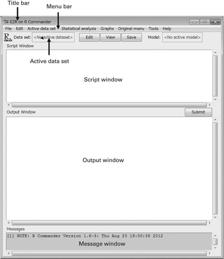
EZR can be started by double-clicking on the shortcut on the desktop or selecting EZR from the ‘Start menu', which causes two windows to appear on the desktop. The window entitled ‘R Console' on the title bar is the main window for R. This window is not used for usual operation in EZR, but should not be closed, as EZR runs on R. The other window entitled ‘EZR on R Commander' is the main operating window for EZR (Figure 1). Functions of EZR can be selected from the menu bar just below the title bar. This menu bar includes the following items: ‘File', ‘Edit', ‘Active data set', ‘Statistical analysis', ‘Graphs', ‘Original menu', ‘Tools' and ‘Help'.

Figure 1.

Main window of EZR.

The user can tell EZR what they would like to do by two methods. First, they can type R commands in the ‘Script window' and click on the ‘Submit' button. The alternative method is easier for beginners. EZR functions can be started by point-and-click access using the items on the menu bar. EZR automatically creates and executes corresponding R commands that appear in the ‘Script window'. Results are shown in the ‘Output window'. If any errors or warnings are noted, messages will appear in the ‘Message window'. The created commands can be saved by selecting ‘File'>‘Save script as' on the menu bar. The output can be saved by selecting ‘File'>‘Save output as'. By saving the commands, users can reproduce the analyses and can also share the procedure with the other investigators.

Creating, modifying and saving an R data set

Windows users can create a new data set directly on EZR by selecting ‘File'>‘New data set'. However, it is more convenient to create a data set using spreadsheet applications such as Microsoft Excel (Microsoft Corporation). Data sets saved as Excel files (.xls or.xlsx) or comma-separated value (CSV) files (.csv) can be imported to EZR by selecting ‘File'>‘Import data'>‘From Excel, Access or dBase data set' or ‘File'>‘Import data'>‘Read Text Data From File, Clipboard or URL', respectively, except that Excel files cannot be imported in EZR on OS X. Alternatively, users can import data by a copy-and-paste approach. Data of interest, copied from a spreadsheet, text file, web site and so on, can be imported into EZR by selecting ‘File'>‘Import data'>‘Read Text Data From File, Clipboard or URL'. Authors should choose ‘Clipboard' for ‘Location of Data file' and ‘Tabs' for ‘Field Separator' on the dialog to paste from a spreadsheet. EZR can also import SPSS data and Stata data.

In the following instructions, a sample data set that includes 93 fictional patients who received Allo-SCT for acute leukemia will be used. The data set file, ‘sample.csv', is available at the http://www.jichi.ac.jp/saitama-sct/SaitamaHP.files/sample.csv. Users can directly import the file into EZR by choosing ‘Internet URL' for ‘Location of Data file' after selecting ‘File'>‘Import data'>‘Read Text Data From File, Clipboard, or URL'. Imported data can be viewed by clicking on the ‘View' button and directly edited by clicking on the ‘Edit' button. The list of variables in the data set can be shown by selecting ‘Active data set'>‘Variables'>‘Show variables in active data set'. In addition, users can create new variables or modify existing variables using the functions under ‘Active data set' on the menu bar. For example, this sample data set has a continuous variable called ‘Age' that represents the patient's age. If a user wants to create a categorical variable, ‘Age40', which has a value of 0 for patients less than 40 years old and 1 for those at least 40 years old, they can select ‘Active data set'>‘Variables'>‘Bin numeric variable with specified threshold'. In the dialog, users can select ‘Age' from the list of numeric variables, input ‘Age40' in the ‘New variable name' column and input ‘40' in the ‘Threshold to bin a numeric variable' column. Alternatively, a new variable can be created by selecting ‘Active data set'>‘Variables'>‘Create new variable'. This function enables more complex computing. For example, if a user wants to create a categorical variable ‘ElderlyMale', which would have a value of 1 for male patients aged at least 60 years old and 0 for other patients, they would input ‘ifelse(Age>=60 & Sex=‘Male', 1, 0)' in the ‘Expression to compute' column in the dialog.

When a categorical variable with more than two categories is to be analyzed in Fine and Gray regression modeling, ‘dummy' variables should be created before analysis, although such ‘dummy' variables are automatically created in multiple regression, logistic regression and Cox proportional hazards regression in R. For example, if a user wants to evaluate the effect of the type of stem cell graft, information for which is included in the categorical variable ‘Source' as ‘BM', peripheral blood ‘PB' and cord blood ‘CB', they would select ‘Active data set'>‘Variables'>‘Create dummy variables' to make three categorical variables named ‘Source.Dummy.BM', ‘Source.Dummy.PB' and ‘Source.Dummy.CB'. ‘Source.Dummy.BM' has a value of 1 for patients who received BM graft and 0 for others. Users should choose one of the three categories as a reference and input dummy variables for the other two categories into the regression model. The effect size, 95% confidence interval and P-value for each category with respect to the reference category will then be shown. If a user directly inputs a categorical variable into multiple regression, logistic regression or Cox proportional hazards regression, the automatically created dummy variables are shown as ‘Source [T.CB]' or ‘Source [T.PB]', for example. The stepwise selection function of explanatory variables based on Akaike information criterion and Bayesian information criterion only accepts these automatically created dummy variables, whereas stepwise selection based on P-value also accepts dummy variables created by a user using EZR. If the option for a ‘Wald test for overall P-value for factors with >2 levels' is selected in the dialog of the regression analyses, the overall P-value for the categorical variable will be calculated.

The modified data set can be saved as an R file (.rda) by clicking the ‘Save' button or selecting ‘File'>‘Active data set'>‘Save active data set'. Only the active data set, as indicated in the column just to the right of ‘Data set:' is saved. The saved data set can be reloaded to EZR by selecting ‘File'>‘Load data set'.

Summarizing data

Descriptive statistics enable the user to glance over features of the data, such as the distribution of or outliers among continuous variables. The proportion of categorical variables is shown by selecting ‘Statistical analysis'>‘Discrete variables'>‘Frequency distributions'. The mean value with the s.d. along with the minimum, median and maximum values of continuous variables are shown by selecting ‘Statistical analysis'>‘Continuous variables'>‘Numerical summaries', but plotting a histogram or a dot chart by selecting ‘Graphs'>‘Histogram' or ‘Dot chart' may be more useful for evaluating the distribution of continuous variables.

A table that shows patient characteristics can be easily created by selecting ‘Statistical analysis'>‘Discrete variables'>‘Create two-way table and compare two proportions'. A grouping variable, ‘Source' for example, should be specified in the ‘Column variable' list and categorical variables that are to be compared among groups should be specified in the ‘Row variable' list. More than one variable can be selected by clicking variables while pressing the ‘Ctrl' key. A summary table will then be shown in the ‘Output window' following the results of statistical tests (Fisher's exact test by default) to compare the proportions of each variable among the groups. A formatted table for presentation can be created by inputting ‘w.twoway()' in the ‘Script window' and clicking on the ‘Submit' button. The table will be copied to the clipboard and can be pasted into a spreadsheet.

Statistical analyses for categorical and continuous variables

Statistical analysis functions for categorical variables, including Fisher's exact test, χ² test, McNemar test, Cochran Q test, Cochran–Armitage test and logistic regression, can be accessed in the ‘Statistical analysis'>‘Discrete variables' menu. Statistical analysis functions for continuous variables, including the Smirnov–Grubbs test, Kolmogorov–Smirnov test, t-test, paired t-test, F-test, Bartlett's test, one-way analysis of variance, multi-way analysis of variance, repeated-measures analysis of variance, analysis of covariance, Pearson's correlation test and linear regression, can be accessed in the ‘Statistical analysis'>‘Continuous variables' menu. Nonparametric tests, including the Mann–Whitney U-test, Wilcoxon's signed rank test, Kruskal–Wallis test, Friedman test, Jonckheere–Terpstra test and Spearman's rank correlation test, are available in the ‘Statistical analysis'>‘Nonparametric tests' menu.

Survival analysis

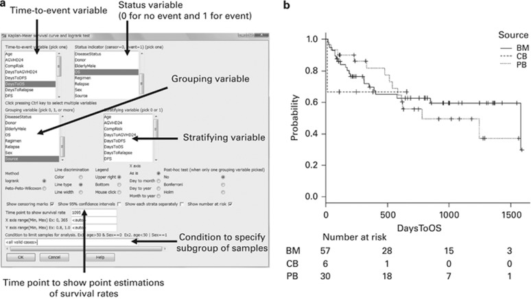
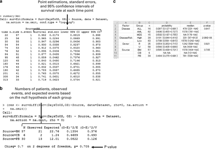
A survival analysis, which is often the primary end point of studies on hematopoietic SCT, can be performed by selecting statistical functions in the ‘Statistical analysis'>‘Survival analysis' menu. For example, users can plot Kaplan–Meier curves and compare survival curves among groups with a log-rank test by selecting ‘Statistical analysis'>‘Survival analysis'>‘Kaplan-Meier survival curve and logrank test'. At least two variables are required: a time-to-event variable, which indicates the time to the occurrence of an event (death in survival analysis) or time to the last evaluation for patients without an event, and a status variable, which has a value of 1 for event and 0 for no event. Users can choose many options in the dialog that mainly involve plotting survival curves (Figures 2a and b). In the ‘Output window', the results of log-rank test can be found following the point estimations with 95% confidence intervals of survival rates (Figures 3a and b). If more than 1 grouping variable is specified, a summary table will be shown, which can be copied to the clipboard by the w.survival() command (Figure 3c).

Figure 2.

(a) Dialog for plotting KM curves and performing a log-rank test. (b) KM curves of overall survival grouped according to the stem cell source.

Figure 3.

(a) Point estimations, s.e. and 95% confidence intervals of survival rate at each time point. (b) The results of log-rank test. (c) Summary of the survival analyses copied to the clipboard and then pasted into a spreadsheet.

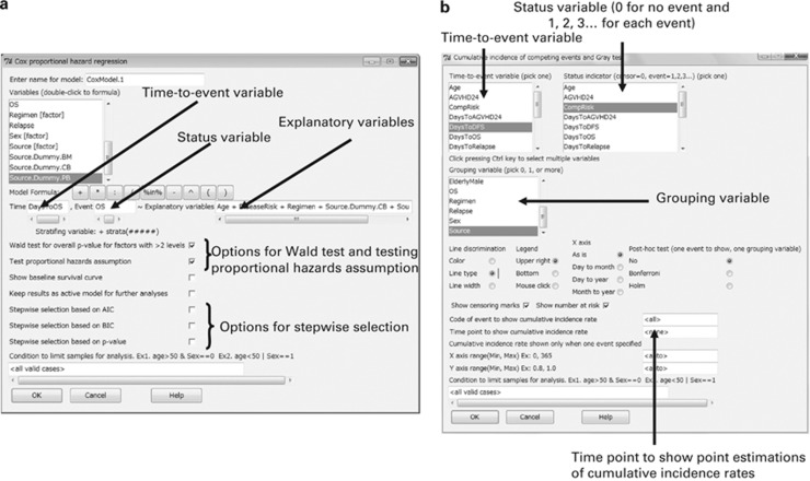
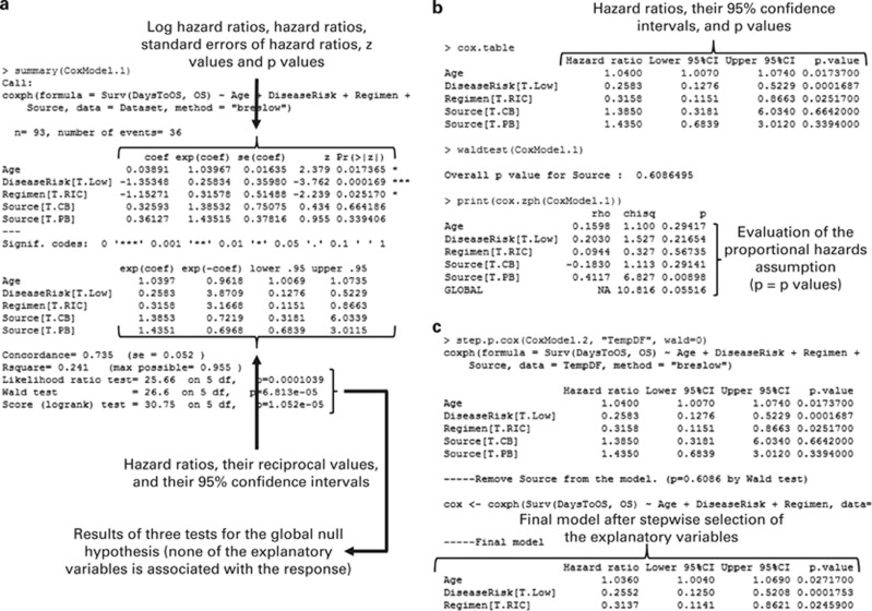
A Cox proportional hazards regression can be performed by selecting ‘Statistical analysis'>‘Survival analysis'>‘Cox proportional hazard regression'. Users have to specify a time-to-event variable, a status variable (1 for event and 0 for no event) and explanatory variables (Figure 4a). In addition, users can choose the following options in the dialog; Wald test for overall P-value for factors with 2 or more levels, test the proportional hazards assumption, show the baseline survival curve and stepwise selection of explanatory variables based on Akaike information criterion, Bayesian information criterion and P-value. In the ‘Output window', the main result of Cox proportional hazard regression can be found that includes the hazard ratios, their 95% confidence intervals and P-values for each explanatory variable, followed by the results of three tests for the global null hypothesis (none of the explanatory variables is associated with the response) (Figure 5a). A summary of proportional hazards regression analysis, the results of Wald test and the results of testing the proportional hazards assumption are shown below the main result (Figure 5b), followed by the results of stepwise selection of explanatory variables (Figure 5c), if requested. The results of a proportional hazards regression analysis can be copied to the clipboard by the w.multi() command. The output of this command reflects the full model and not the model after stepwise selection of explanatory variables. Survival curves adjusted for other factors by the mean of covariates method, in which average values of covariates are entered into the Cox proportional hazards model, can be drawn by selecting ‘Graphs'>‘Adjusted survival curve'.

Figure 4.

(a) Dialog for performing a Cox proportional hazards regression. (b) Dialog for plotting cumulative incidence curves and performing Gray's test.

Figure 5.

(a) Main result of Cox proportional hazard regression that includes the hazard ratios, their 95% confidence intervals and P-values for each explanatory variable, followed by the results of three tests for the global null hypothesis. (b) Summary of proportional hazards regression analysis, the results of Wald test and the results of testing the proportional hazards assumption. (c) Results of stepwise selection of explanatory variables.

A TD covariate can be incorporated in the Cox proportional hazards regression in EZR. However, the function is limited to a simple TD covariate. EZR can handle only one TD covariate, which is initially 0 and may change to a value of 1 thereafter. For example, if a user wants to evaluate the impact of grade II–IV acute GVHD on survival, it is not appropriate to treat the development of acute GVHD as if it were known before transplantation, as patients who died or relapsed before the development of GVHD would be included in the ‘no GVHD group'. A variable whose value may change after transplantation should be treated as a TD covariate, and this can be performed in EZR by selecting ‘Statistical analysis'>‘Survival analysis'>‘Cox proportional hazard regression with time-dependent covariate'. In this case, ‘AGVHD24', which has a value of 1 for patients who developed grade II–IV acute GVHD, should be selected in the ‘TD covariate' list. ‘DaysToAGVHD24', which is the time from transplantation to the development of grade II–IV acute GVHD for patients who developed grade II–IV acute GVHD or the time to the last evaluation for patients who did not develop grade II–IV acute GVHD, should be specified in the ‘Time when TD covariate changes from 0 to 1' list. Other explanatory variables should be specified in the same manner with Cox proportional hazard regression, as described above. In the ‘Output window', the effect of grade II–IV acute GVHD will be shown in the row ‘covariate_td'.

Competing risk analysis

A competing risk analysis is an important statistical function in studies on hematopoietic SCT. For example, if an investigator wants to analyze the cumulative incidence of relapse after transplantation, death without relapse (non-relapse mortality) precludes the occurrence of relapse. Previously, one minus the Kaplan–Meier (1−KM) method of relapse while treating deaths without relapse as censored observations has been used to estimate the incidence of relapse. However, this analysis overestimates the incidence of relapse, as it attempts to predict the incidence of relapse when patients who actually die would have relapsed. As a result, the sum of the incidence of relapse, the incidence of non-relapse mortality and the probability of relapse-free survival exceeds 100%. A more appropriate estimate can be obtained using the cumulative incidence function. This method subdivides the probability of failure into the probability corresponding to each competing event and provides an accurate incidence for each event. The statistical significance of the difference in the cumulative incidences of competing events among groups can be assessed by Gray's test.⁹ In addition, regression models for competing risks data have been proposed by Fine and Gray,¹⁰ and by Klein and Anderson.¹¹

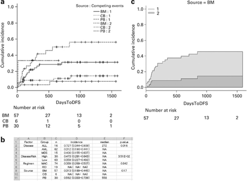
These competing risk analyses can be provided by adding the ‘cmprsk' package to R.⁶ Excellent instructions for the use of this package have been provided in this journal by Scrucca et al. in 2007 and 2010.^{12, 13} EZR makes it possible to access these analyses in a point-and-click manner. For example, the cumulative incidences of relapse and non-relapse mortality can be plotted and compared among groups by selecting ‘Statistical analysis'>‘Survival analysis'>‘Cumulative incidence of competing events and Gray test' (Figure 4b). Users have to specify a time-to-event variable (‘DaysToDFS' in this case, which indicates the time to the earliest event or time to the last evaluation for patients without any events), a status indicator (‘CompRisk', which has a value of 1 for relapse, 2 for non-relapse mortality and 0 for no event), and grouping variables, if required (‘Source' in this case). The ‘Output window' shows the results of Gray's test following the point estimations with 95% confidence intervals of the cumulative incidences of each event. If a user wants to plot cumulative incidence curves for only one of the competing events, the number of event that corresponds to the event of interest should be specified in the ‘Code of event to show cumulative incidence rate' column in the dialog. If more than 1 grouping variable is specified and only one of the events is specified in the ‘Code of event to show cumulative incidence rate' column, a summary table will be shown, which can be copied to the clipboard by the w.ci() command (Figure 6b). A graph that shows the cumulative incidences in a stacked manner can be plotted by selecting ‘Graphs'>‘Stacked cumulative incidences' (Figure 6c).

Figure 6.

(a) Cumulative incidence curves of relapse (event=1) and non-relapse mortality (event=2) grouped according to the stem cell source. (b) Summary of the cumulative incidence analyses copied to the clipboard and then pasted into a spreadsheet. (c) Stacked cumulative incidence graph. The light gray area indicates the incidence of relapse (event=1) and the dark gray area indicates the incidence of non-relapse mortality (event=2).

Fine and Gray regression modeling can be performed from the menu, ‘Statistical analysis'>‘Survival analysis'>‘Fine-Gray proportional hazard regression for competing events'. Users have to specify a time-to-event variable, a status variable, the number of event corresponding to the event of interest and explanatory variables. The results of a regression analysis can be copied to the clipboard by the w.multi(crr.table) command. When we consider the sample file, if the effect of the use of PB or CB compared with BM on the incidence of relapse is evaluated by adjusting for age, disease risk and conditioning regimen, the use of PB as stem cell graft is significantly associated with an increased incidence of relapse with a subdistribution hazard ratio of 2.37 (95% confidence interval: 1.11–5.04; P=0.025). However, this result should be considered with caution, as the overall P-value for stem cell graft was 0.070 by the Wald test, which can be calculated by checking this option in the dialog.

I should note that the log-rank test and Cox proportional hazards regression are also valid analyses of competing risks data. In these analyses, cause-specific hazard function is evaluated instead of the cumulative incidence function, censoring events other than the event of interest. Therefore, the time-to-event variable should indicate the time to the earliest event or time to the last evaluation for patients without any events, and the status variable should have a value of 1 for event of interest and 0 for other events or no event. The choice and interpretation of these statistical tests for competing risks data are discussed elsewhere.¹⁴

Final remarks

In addition to the functions introduced above, EZR enables the analysis of diagnostic tests in the ‘Statistical analysis'>‘Accuracy of diagnostic test' menu, matched-pair analysis in the ‘Statistical analysis'>‘Matched-pair analysis' menu, meta-analysis in the ‘Statistical analysis'>‘Metaanalysis and metaregression' menu and a sample size calculation in the ‘Statistical analysis'>‘Calculate sample size' menu. A variety of graphs can be accessed in the ‘Graphs' menu and the statistical functions that were included in the original R commander can be found in the ‘Original menu'. Created graphs can be copied to the clipboard from the menu of the graph window, ‘File'>‘Copy to the clipboard', either as a bitmap or as a metafile. I hope that EZR will help researchers to perform statistical analyses, especially in clinical studies on hematopoietic SCT.

The author declares no conflict of interest.

References

- The popularity of data analysis software. . http://r4stats.com/articles/popularity/ (Accessed 1 August 2012).
- Klein JP, Rizzo JD, Zhang MJ, Keiding N. Statistical methods for the analysis and presentation of the results of bone marrow transplants. Part I: unadjusted analysis. Bone Marrow Transplant. 2001;28:909–915. doi: 10.1038/sj.bmt.1703260. [DOI] [PubMed] [Google Scholar]
- Klein JP, Rizzo JD, Zhang MJ, Keiding N. Statistical methods for the analysis and presentation of the results of bone marrow transplants. Part 2: regression modeling. Bone Marrow Transplant. 2001;28:1001–1011. doi: 10.1038/sj.bmt.1703271. [DOI] [PubMed] [Google Scholar]
- Labopin M, Iacobelli S.Statistical guidelines for EBMT. http://portal.ebmt.org/sites/clint2/clint/Documents/StatGuidelines_oct2003.pdf (Accessed 1 August 2012).
- The Comprehensive R Archive Network . http://cran.r-project.org/ (Accessed 1 August 2012).
- Rcmdr: R Commander . http://cran.r-project.org/web/packages/Rcmdr/index.html (Last accessed on 1 August 2012).
- Kanda Y.Free statistical software: EZR (Easy R) on R commander. http://www.jichi.ac.jp/saitama-sct/SaitamaHP.files/statmedEN.html (Accessed 1 August 2012).
- Kanda Y.EZR de yasashiku manabu toukeigaku: EBM no jissen kara rinsho-kenkyu made[in Japanese]. Chugai Igakusha: Tokyo, Japan; 2012 [Google Scholar]
- Gray RJ. A class of k-sample tests for comparing the cumulative incidence of a competing risk. Ann Statist. 1988;16:1141–1154. [Google Scholar]
- Fine JP, Gray RJ. A proportional hazards model for subdistribution of a competing risk. J Am Stat Assoc. 1999;94:456–509. [Google Scholar]
- Klein JP, Andersen PK. Regression modeling of competing risks data based on pseudovalues of the cumulative incidence function. Biometrics. 2005;61:223–229. doi: 10.1111/j.0006-341X.2005.031209.x. [DOI] [PubMed] [Google Scholar]
- Scrucca L, Santucci A, Aversa F. Competing risk analysis using R: an easy guide for clinicians. Bone Marrow Transplant. 2007;40:381–387. doi: 10.1038/sj.bmt.1705727. [DOI] [PubMed] [Google Scholar]
- Scrucca L, Santucci A, Aversa F. Regression modeling of competing risk using R: an in depth guide for clinicians. Bone Marrow Transplant. 2010;45:1388–1395. doi: 10.1038/bmt.2009.359. [DOI] [PubMed] [Google Scholar]
- Dignam JJ, Kocherginsky MN. Choice and interpretation of statistical tests used when competing risks are present. J Clin Oncol. 2008;26:4027–4034. doi: 10.1200/JCO.2007.12.9866. [DOI] [PMC free article] [PubMed] [Google Scholar]