A Robust Method for Transcript Quantification with RNA-Seq Data

Abstract

The advent of high throughput RNA-seq technology allows deep sampling of the transcriptome, making it possible to characterize both the diversity and the abundance of transcript isoforms. Accurate abundance estimation or transcript quantification of isoforms is critical for downstream differential analysis (e.g., healthy vs. diseased cells) but remains a challenging problem for several reasons. First, while various types of algorithms have been developed for abundance estimation, short reads often do not uniquely identify the transcript isoforms from which they were sampled. As a result, the quantification problem may not be identifiable, i.e., lacks a unique transcript solution even if the read maps uniquely to the reference genome. In this article, we develop a general linear model for transcript quantification that leverages reads spanning multiple splice junctions to ameliorate identifiability. Second, RNA-seq reads sampled from the transcriptome exhibit unknown position-specific and sequence-specific biases. We extend our method to simultaneously learn bias parameters during transcript quantification to improve accuracy. Third, transcript quantification is often provided with a candidate set of isoforms, not all of which are likely to be significantly expressed in a given tissue type or condition. By resolving the linear system with LASSO, our approach can infer an accurate set of dominantly expressed transcripts while existing methods tend to assign positive expression to every candidate isoform. Using simulated RNA-seq datasets, our method demonstrated better quantification accuracy and the inference of dominant set of transcripts than existing methods. The application of our method on real data experimentally demonstrated that transcript quantification is effective for differential analysis of transcriptomes.

1. Introduction

Recent studies have estimated that as many as 95% of all multi-exon genes are alternatively spliced, resulting in more than one transcript per gene (Pan et al., 2008; Wang et al., 2008). Transcript quantification determines the steady state levels of alternative transcripts within a sample, enabling the detection of differences in the expression of alternative transcripts under different conditions. Its application in detecting biomarkers between diseased and normal tissues can greatly impact biomedical research.

High-throughput sequencing technology (e.g., RNA-seq with Illumina, ABI Solid, etc.) provides deep sampling of the mRNA transcriptome. It allows the parallel sequencing of a large number of mRNA molecules, generating tens of millions of short reads with lengths up to 100 bp at one end or both ends of mRNA fragments. Recent studies using RNA-seq have significantly expanded our knowledge on both the variety and the abundance of alternative splicing events (Brosseau et al., 2010; Wu et al., 2011).

However, transcript quantification remains a challenging problem. First, it is commonly observed that “the more the isoforms, the harder to predict” (Li et al., 2011). Intuitively, transcript isoforms from the same gene often overlap significantly, and a short read may be mapped to more than one transcript isoform. Determining the expression of individual transcripts from short-read alignment, therefore, can lead to an unidentifiable model, where no unique solution exists. Secondly, transcript quantification often takes the candidate set of transcript isoforms, either from annotation databases such as Ensembl (Flicek et al., 2012) and Refseq (Pruitt et al., 2007), or inferred from the splice graph using programs like Scripture (Guttman et al., 2010), IsoInfer (Feng et al., 2010), IsoLasso (Li et al., 2011), or Cufflinks (Trapnell et al., 2010). It is biologically unlikely to expect all candidate transcripts for a given gene to be significantly expressed concurrently in a cell. However, existing analytical approaches tend to assign positive expression values to every candidate transcript provided, thereby creating a situation in which large errors in abundance estimation can be computationally introduced for transcript isoforms that may, in reality, barely be expressed. An improved transcript quantification method, therefore, would determine or logically infer the subset of expressed transcript isoforms. Finally, various sampling biases have been observed regularly in RNA-seq datasets as a result of library preparation protocols. These biases typically include position-specific bias (Bohnert and Rätsch, 2010; Li et al., 2010; Roberts et al., 2011; Wu et al., 2011) such as 3’ bias and transcription start and end biases, and sequence-specific bias (Li et al., 2010; Roberts et al., 2011; Turro et al., 2011), where the read sampling in the transcriptome favors certain subsequences. How to compensate for these biases during transcript quantification is an open problem.

Transcript isoforms can differ not only in exons alternatively included or excluded but also where two or more exons are connected together. In RNA-seq data, this information is typically implied by the spliced reads, (i.e., the reads that cross one or more splice junctions). We have developed a general linear model for transcript quantification that leverages discriminative features in spliced reads to ameliorate the issue of identifiability and simultaneously corrects the sampling bias. Our contribution in this paper is three-fold: (1) We explicitly identify MultiSplice, a novel structural feature consisting of a contiguous set of exons that are expected to be spanned by the RNA-seq reads or transcript fragments of a given length. The MultiSplice, which includes single splice junctions as a special case, is used in two ways: its presence in the sample will infer the host transcript while its absence may reject it. MultiSplices are more powerful than single exons in disambiguating transcript isoforms, making more transcript quantification problems identifiable with long or paired-end reads. (2) We set up a linear system that minimizes the summed relative squared errors regarding the ratio of the expected expression against the observed expression across all structure features along a gene while taking into account various bias effects: (3) We develop an iterative minimization algorithm in combination with LASSO (Tibshirani, 1996) to resolve the aforementioned linear system in order to achieve the most accurate set of dominantly expressed transcripts while simultaneously correcting biases.

We have demonstrated the efficacy of our methods on both simulated RNA-seq datasets and real RNA-seq data: (1) We conducted the first study to investigate the question: What is the maximum read length needed in order to disambiguate all possible transcript isoforms in transcriptomes from different species; (2) we compared the proposed method with several state-of-the-art methods including Cufflinks, RSEM, the Poisson model, and the ExonOnly model. Our results using simulated data from the human mRNA transcriptome demonstrated superior performance of the proposed method in most cases. When applied to eight RNA-seq datasets from two breast cancer cell lines (MCF-7 and SUM-102), the quantification obtained from MultiSplice demonstrated good consistency within technical replicates from each transcriptome-wide assessment and substantial differences between the two biological groups (cell lines) in a small percentage of genes.

2. Related Work

Various transcript quantification algorithms have been published recently. These methods can be divided mainly into two categories: read-centric and exon-centric. The representative methods using read-centric approaches include, but are not limited to, Cufflinks (Trapnell et al., 2010), IsoEM (Nicolae et al., 2011), and RSEM (Li and Dewey, 2011). The central idea with read-centric approaches is to assign probability for each fragment to one transcript by maximizing the joint likelihood of read alignments based on the distribution of transcript fragments, and thereby estimating the transcript expression. When it is impossible to precisely allocate a fragment to a unique transcript, Cufflinks, for example, simply disregards or randomly assigns the read, causing information loss or inaccurate quantification. The second strategy, called exon-centric, considers the read abundance on an exonic segment as the cumulative abundance of all transcript isoforms. Methods in this category represent the transcript as a combination of exons and aim at estimating individual transcript abundance from the observed read count or read coverage at each exon. The representative models in this category include the Poisson model (Jiang and Wong, 2009; Richard et al., 2010; Srivastava and Chen, 2010) and linear regression approaches, such as rQuant (Bohnert and Rätsch, 2010), IsoLasso (Li et al., 2011), and SLIDE (Lia et al., 2011).

Transcript abundance estimations can be unidentifiable, where no unique quantification exists. Both exon-centric and read-centric models may suffer from this problem. The article by Lacroix et al. (2008) is one of the theoretical studies that have considered the identifiability problem of transcript quantification.

3. Methods

In this section, we propose a method designated MultiSplice, for mRNA isoform quantification. We first define the observed features used in the MultiSplice model and the statistics collected. Then, we derive a general linear model to relate transcript-level estimate to the observed expression on every feature.

Preliminaries. For a gene g, we use to denote the set of exonic segments (Jiang and Wong, 2009; Li et al., 2011) in g, which are disjoint genomic intervals on the genome that can be included in a transcript in its entirety. We use to denote the set of mRNA isoforms transcribed from g. These mRNAs can be a set of annotated transcripts retrieved from a database such as Ensembl (Flicek et al., 2012) or Refseq (Pruitt et al., 2007). A transcript is defined by a sequence of exon segments, , where and n_t denotes the number of exonic segments in the transcript t. The length of each exonic segment e is defined as the number of nucleotides in the exonic segment, denoted as l(e). Hence, the length for every transcript is .

3.1. MultiSplice

In a typical RNA-seq dataset, a significant percentage of the read alignments are spliced alignments that connect more than one exon. With paired-end reads, the transcript fragment where its two ends are sampled can be inferred based on the distribution of the insert size (Roberts et al., 2011). Transcript fragments are typically between 200 bp and 300 bp, making them more likely to cross multiple exons, indicating these exons are present together in one transcript. This information can be crucial in distinguishing alternative transcript isoforms. However, they are often ignored in current computational approaches.

In this subsection, we consider a sequence of adjacent exons in an mRNA transcript covered by transcript fragments. These structural features are the basis of MultiSplice. For generality, we assume that the RNA-seq reads are sampled from transcript fragments whose lengths follow a given distribution F_fr with probability density function f_fr. For example, the fragment-length distribution F_fr is often modeled as a normal distribution with mean and variance learned from the genomic alignment of the RNA-seq reads. We also assume the maximum fragment length is l_fr.

Definition 1. Let be a substring of a transcript sequence , n_b ≥ 1 and i + n_b ≤ n_t. Then b is a MultiSplice in t if and only if

(1)

The condition in Equation 1 guarantees that a MultiSplice b connects n_b + 1 adjacent exons with at least one base landed on the 5’ most exon and the 3’ most exon . We use to denote the set of all MultiSplices in gene g. From the definition, the set of MultiSplices vary according to the fragment length l_fr. The longer the fragments, the more MultiSplices are expected to function as structural features, and the higher power in disentangling highly similar alternative isoforms.

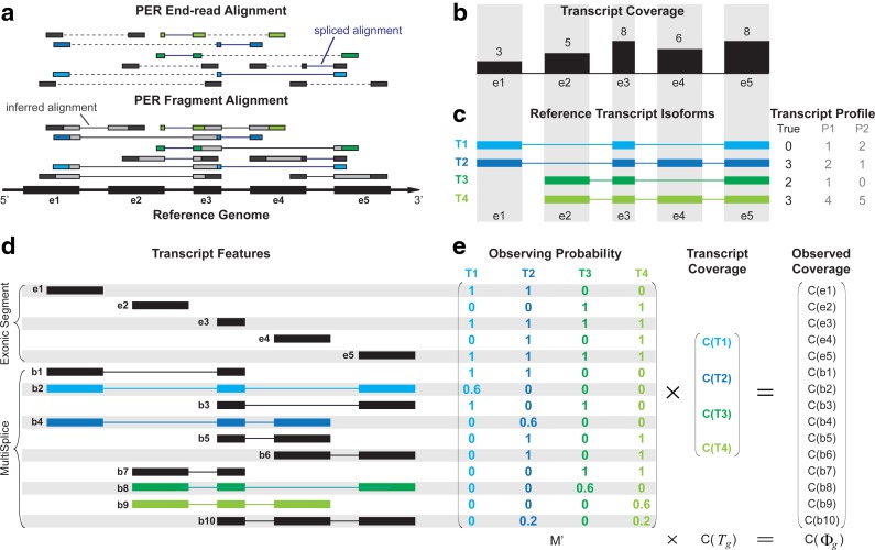
In Figure 1, for example, assume the maximum fragment length is l_fr = 300 bp with the expected fragment length of 250 bp and the exonic segments of this gene have lengths of l(e₁) = 200 bp, l(e₂) =200 bp, l(e₃) = 100 bp, l(e₄) = 200 bp, l(e₅) = 200 bp. In reference transcript T₁ = e₁e₃e₅, b₂ = e₁e₃e₅ is a substring of T₁, and we have l(e₃) = 100 bp < 300 bp = l_fr, which allows a fragment to cover b₂. Therefore, b₂ is a MultiSplice feature of the gene. Combining MultiSplices from all the reference transcripts, b₁, b₃, b₅, b₆, and b₇ are MultiSplices consisting of a single splice junction, b₂, b₄, b₈, b₉, and b₁₀ are MultiSplices consisting of two splice junctions.

FIG. 1.

Overview of the MultiSplice model. (a) Sequenced RNA-seq short-reads are first mapped to the reference genome using an RNA-seq read aligner such as MapSplice (Wang et al., 2010). In the presence of paired-end reads, MapPER (Hu et al., 2010) can be applied to find PER fragment alignments for the entire transcript fragment based on the distribution of insert size. (b) Observed coverage on each exonic segment. (c) Four transcripts originate from the alternative start and exon-skipping events. Provided with these transcripts, abundance estimates would be unidentifiable for methods that only use coverage on exonic segments. Both transcript profiles P₁ and P₂, for instance, can explain the observed read coverage on each exon but deviate from the true transcript expression profile. (d) MultiSplices that connect multiple exonic segments in a transcript. (e) A linear model can be set up where the expected coverage on every exonic or MultiSplice feature approximates its observed coverage. The transcript expression is solved as the one that minimizes the sum of squared relative error.

3.2. Expected coverage and observed coverage

Given the gene g and a transcript , let c_i be the number of transcript fragments covering the ith nucleotide of t. We define the coverage on t as the averaged number of transcripts covering each base in the transcript, . Then C(t) is an estimator for the quantity of t in the sample, which provides a direct measure for the expression level of t. In our model, C(t) is the unknown variable. The feature space that can be observed from the given RNA-seq sample is the union of all exonic segments and MultiSplices of the gene, . We aim at resolving the transcript expressions that minimize the difference between the observed expression and the expected expression of every feature.

The observed coverage on an exonic segment is defined as , where c_i is the number of reads covering the ith nucleotide in e. The read coverage C(e) provides an estimator for the number of transcript copies that flow through the exonic segment e assuming uniform sampling. For a MultiSplice , we use C(b) to denote the read coverage on b defined as the number of transcript fragments that include b.

For every and every transcript , the expected coverage of feature φ from t can be expressed as a function of the transcript quantity C(t), that is, E[C(φ|t)] = m(φ,t)C(t), where m(φ,t) contains the probability of observing φ in t assuming uniform sampling. Next, we define the expected coverage on exonic segments and MultiSplice respectively.

For an exonic segment e in t, assuming N_t fragments were sampled from t, the number of fragments falling in e then follows a binomial distribution with parameters N_t and p(e|t), where denotes the probability that a fragment sampled from t originated from e. Therefore, the expected number of reads on e from t is E[N_e|t] = N_tp(e|t). Let be the fragments sampled on t, the expected fragment coverage on t is , where E[l(fr)] is the expected fragment length. On the other hand, the expected fragment coverage on e contributed by t is calculated as . Since . Therefore, we could get , which means the expected fragment coverage on e contributed by t equals the expected fragment coverage of t, which concludes that the probability of observing e in t is 1: m(e, t) = 1.

For a MultiSplice , we are interested in the number of fragments containing it. Should a transcript fragment fr cover b, fr must start no later than the 3’ end boundary of the 5’ most exonic segment and have at least one base landed on the 3’ most exonic segment . Therefore, there exists a window w(b) before the 3’ end of with length , where b can be covered by the transcript fragment fr. The probability that fr covers b in transcript t is hence . Equivalent to the expected number of fragments from t that contain b, the expected fragment coverage on b from t is . Since E[C(b|t)] = m(b,t)C(t), the probability that the MultiSplice b is observed within transcript t is . Recall that , therefore, . In Figure 1, for example, .

In summary, the probability that a feature φ contained in a uniformly sampled transcript fragment f_r is:

(2)

with φ ⊂ t standing for that φ is contained in t.

3.3. A generalized linear model for transcript quantification

We construct a matrix to represent the structure of the transcripts, whose entry on the row of φ and the column of t corresponds to the probability of observing feature φ from transcript t, M′(φ, t) = m(φ, t). The linear model is set up for every feature by equating the observed coverage on φ to the expected coverage from all transcripts:

(3)

Here C(t) ≥ 0 for every is the error term for feature φ in transcript t.

Lemma 1. The MultiSplice model for transcript quantification is identifiable if the rank of M′ is no less than the number of transcripts .

Lemma 1 directly follows the the Rouché-Capelli theorem (Horn and Johnson, 1990).

4. Bias Correction

Under uniform sampling, the sampling probability is the same at every nucleotide of a transcript. The observed coverage on φ is unbiased for the expected coverage on t. In this case, the bias coefficient σ(φ, t) is set to 1 for all transcripts and features. However, sampling bias is often introduced in RNA-seq sample preparation protocols and has been demonstrated to have significant effects in RNA-seq analysis (Kozarewa et al., 2009; Wang et al., 2009). Therefore, we discuss in the following subsections how MultiSplice corrects various sampling bias via learning of the bias coefficients and simultaneously solves the linear model for transcript coverage C(t) of every transcript t.

Figure 2a–e shows how various types of sampling bias alter the sampling probability and hence the coverage. Two types of sampling bias are commonly observed in RNA-seq data, namely, the position-specific bias and the sequence-specific bias (Bohnert and Rätsch, 2010; Olejniczak et al., 2010; Srivastava and Chen, 2010; Roberts et al., 2011). In our model, sampling bias may affect the sampling probability of both the exonic segments and MultiSplices. Therefore, we calculate the bias coefficient σ(φ,t) for every feature and every transcript t so that E[C(φ|t)] = σ(φ, t)m(φ, t)C(t). Next, we introduce each independent bias individually.

FIG. 2.

Sampling bias present in the RNA-seq data. (a) RNA-seq read coverage under uniform sampling. (b) RNA-seq read coverage under uniform sampling with transcript start/end bias. (c) RNA-seq read coverage under uniform sampling with sequence-specific bias. (d) RNA-seq read coverage under uniform sampling with 5’/3’ position-specific bias. (e) RNA-seq read coverage under uniform sampling with all aforementioned types of bias. (f) Sampling bias on gene CENPF in the breast-cancer dataset used in Section 6. Please note that the second peak in the coverage plot is not an exon in CENPF. The observed coverage on each exon decreases almost linearly from the 3’ end to the 5’ end. The coverage also drops at the bases near the end of the gene. The nonuniformity in the two middle large exons is likely to be due to the sequence-specific sampling bias.

Sequence-specific bias. The sequence-specific bias refers to the perturbation of sampling probability related to certain sequences at the beginning or end of the transcript fragments (Li et al., 2010; Roberts et al., 2011). The characteristic of this type of bias in the given RNA-seq sample can be learned in advance by examining the relationship between GC content and the observed coverage on single-isoform genes. To derive the sequence-specific bias at an arbitrary exonic position, we look into 8 bp upstream to the 5’ start to 11 bp downstream according to Roberts et al. (2011). A Markov chain is constructed to model the effect on the sampling probability at the position from the sequence of surrounding nucleotides. Then we use an approach based on the probabilistic suffix tree (Bejerano, 2004) to learn the sequence-specific bias coefficient α(t, i) for ith nucleotide in transcript t.

Transcript start/end bias. Sampling near transcript start site or transcript end site is often insufficient. The read coverage in these regions is typically lower than expected because the positions where a sampled read can cover are restricted by the transcript boundaries. The bias coefficient for start/end bias at the ith nucleotide in transcript t is written as:

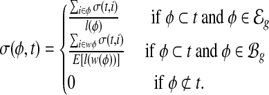
5’/3’ position-specific bias. Position-specific bias refers to the alteration on sampling probability according to position in the transcript. For example, nucleotides to the 3’ end of the transcript have higher probability to be sampled in Figure 2f. Here we model the position-specific bias coefficient as a linear function, . The intercept gives the bias coefficient at the 5’ transcript start site. The slope measures the extent of the bias: a positive indicates that 3’ transcript end site has higher sampling probability than the start site; a zero indicates no positional bias in the transcript t.

Combined bias model. Assuming the above three types of bias have independent effect on read sampling, we derive the bias coefficient at ith nucleotide in transcript t as σ(t, i) = α(t, i) · β(t, i) · γ(t, i). The bias coefficient of an exonic segment is then the averaged bias coefficient on all positions in the exonic segment e, and the bias coefficient of a MultiSplice is the averaged bias coefficient on all positions in its sampling window w(b). In summary, the bias coefficient for a MultiSplice feature in transcript t is

(4)

5. Solving The General Linear Models With Bias Correction

Conventionally, we are interested in the set of transcript expressions that minimize the sum of squared errors, the absolute residuals between the expected coverage and the observed coverage. This solution is relatively sensitive to unexpected sampling noise that often occurs in real RNA-seq samples and may lead to a highly unstable extrapolation when the expression of the alternative splicing events discriminating the transcripts is notably lower than the average level of gene expression. Therefore, we define the sum of squared relative errors (SSRE), which measures the relative residual regarding the ratio of the expected coverage against the observed coverage.

(5)

Bias parameter estimates. Among all the bias parameters, the sequence-specific bias is learned in advance while the start and end bias is a function of transcript fragment length. The only bias parameters unknown related to the 3’ bias are defined by the intercept and slope for every transcript . Therefore, we use an iterative-minimization strategy and search for a set of bias coefficients 's and 's that better fit the RNA-seq sample than the uniform sampling model. We start with the transcript coverage C(t)'s that are solved from the uniform sampling model (with and as initial condition). Analogous to the hill-climbing algorithm (Russell and Norvig, 2003), we then iteratively probe a locally optimal set of transcript coverage together with the bias coefficients around the uniform solution through minimizing the SSRE. In each iteration, a candidate solution is obtained through sequentially setting the partial derivatives to 0 with respect to every unknown parameter , and for every transcript . If the candidate solution results in a smaller SSRE, the candidate solution is taken and the iteration continues. For details of the step to estimate the bias parameters, please refer to the Appendix section.

Solving the linear model with LASSO regularization. Lastly, we solve for the level of individual transcript expression with additional regularization, based on the bias coefficients from the previous step. One common problem in transcript quantification is that the set of expressed transcripts are not known a priori. Hence it becomes crucially important to identify the set of truly expressed transcripts provided in a candidate set. Therefore, we further apply the L1 regularization (known as LASSO) for its proven effectiveness in irrelevance removal and solve for the set of transcript expression that minimizes the following loss function

(6)

where λ ≥ 0 denotes the weight of the L1 shrinkage and C(t) ≥ 0 for every .

6. Experimental Results

To evaluate the performance of the MultiSplice model, we compared it with four other approaches. The ExonOnly model, where only exonic segments are used to represent transcript composition as proposed in SLIDE (Lia et al., 2011), was implemented using a linear regression approach with LASSO. The ExonOnly model provided the baseline comparison for MultiSplice. The Poisson model, which was originally proposed by Richard et al. (2010), was implemented in C. Two read-centric models are analyzed: Cufflinks (Trapnell et al., 2010), which uses the reads aligned to the reference genome, and RSEM (Li and Dewey, 2011), which uses the reads aligned to the set of reference transcript sequences. Cufflinks 1.1.0 was downloaded from its website in September 2011. RSEM 1.1.13 was downloaded in November 2011.

These algorithms were run on both simulated datasets and real datasets. Reads were first mapped by MapSplice 1.15.1 (Wang et al., 2010) to the reference genome. If the read was paired-end, MapPER (Hu et al., 2010) was applied to infer the alignment of the entire transcript fragment.

6.1. Transcriptome identifiability with increasing read length

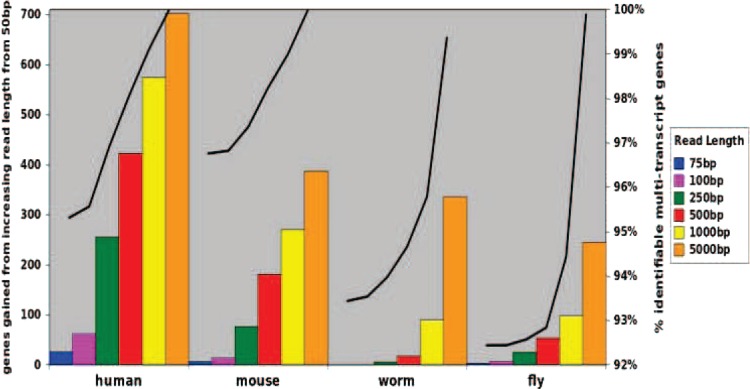
We first study how the increase in read length may alleviate the lack of identifiability issues in transcript quantification using MultiSplice. We downloaded University of California, Santa Cruz (UCSC) gene models in human (track UCSC Genes:GRCh37/hg19), mouse (track UCSC Genes:NCBI37/mm9), worm (track WormBase Genes:WS190/ce6), and fly (track FlyBase Genes:BDGP R5/dm3). We computed the feature matrix used in MultiSplice given variable read length and determined its rank. The transcript isoforms of a gene is identifiable if the rank of the feature matrix is no less than the number of transcripts. Figure 3 plots the additional number of genes that become identifiable as the read length increases from 50 bp assuming single-end read RNA-seq data. For all four species, as the read length increases, MultiSplice is capable of resolving the transcript quantification issues of more genes. With 500 bp reads, about 98% genes in both human and mouse become identifiable. Surprisingly, for worm and fly, 500 bp reads do not gain significant improvement over 50 bp reads. This is mostly due to the fact that the exon lengths of fly and worm are comparably much longer (Kristi et al., 2005) than human and mouse, making it difficult for reads of moderate size to take effect. With current short-read technology, where read length is typically 100 bp or less, paired-end reads with the size of transcript fragments around 500 bp may be the most economical and effective for transcription quantification for genes with identifiability issues. This is under the assumption that it is possible to infer the transcript fragment from paired-end reads based on the tightly controlled distribution of insert size.

FIG. 3.

Changes in mRNA identifiability as a function of transcript fragment/read length. Starting from levels achieved with 50-bp single-end reads, the left side of the y-axis shows the additional number of genes that become identifiable using MultiSplice as the read length increases. The y-axis on the right side shows the total percentage of genes for which mRNA transcript structures are resolved. The UCSC annotated transcript sets of four species: human, mouse, fly, and worm were used for this analysis.

6.2. Simulated human RNA-seq experiment

Data simulation. Due to the lack of the ground truth within real datasets, simulated data has become an important resource for the evaluation of transcript quantification algorithms (Bohnert and Rätsch, 2010; Li et al., 2010; Nicolae et al., 2011). We developed an in-house simulator to generate RNA-seq datasets of a given sampling depth using UCSC human hg19 annotation. The simulation process consists of three steps: (1) Randomly assign relative proportions to all the transcripts within a gene and set this as the true profile; (2) calculate the number of reads to be sampled from each transcript; and (3) sample transcript fragments of a given length along the transcripts according to the per-base coefficient for the ith base on transcript t, where α(t, i) and β(t, i) are the sequence-specific bias and the transcript start/end bias as defined in Section 4, and k is the slope of the position-specific bias. Paired-end reads will be generated by taking the two ends of the transcript fragment. Please note the sequence bias per base has been learned from a real dataset, a technical replicate of MCF-7 data that will be introduced in the next section.

Accuracy measurement. Due to inconsistencies in the normalization scheme used by different software, the estimated abundance may not be comparable among different approaches. Hence, we computed relative proportions of transcript isoforms for each method. The similarity between the estimated result and the ground truth is measured by both Pearson correlation and Euclidean distance. Pearson correlation is the accuracy measurement used in rQuant (Bohnert and Rätsch, 2010). Let X denote the vector of real isoform proportions of a gene and denote the estimated proportions. The formula of the correlation is: . A value close to 1 means that our estimation is highly accurate and vice versa. Below, we adopt a boxplot to illustrate the performance of each method. The box is constructed by the first quartile, the median, and the third quartile. The ends of the upper and lower whisker are given by the third quartile +1.5 × IQR(inner quartile range) and first quartile −1.5 × IQR, respectively. Due to the space limit, we present the result of correlation measurement in the main manuscript. Results measured by Euclidian distance can be found in the Appendix section.

Varying read lengths. On the premise of the same sequencing depth, we would like to find out whether or not the read length will affect the estimation results. Forty million RNA-seq fragments were simulated from the human transcriptome; 2x50-bp paired-end reads (insert size around 150-bp) were generated from these fragments. A 50-bp single-end read set was constructed by simply throwing out the second read of each pair and the 100-bp single reads were obtained by taking the 100-bp prefix of the transcript fragments. This configuration allows a fair evaluation about the effect of varying read lengths by eliminating difference from random read sampling.

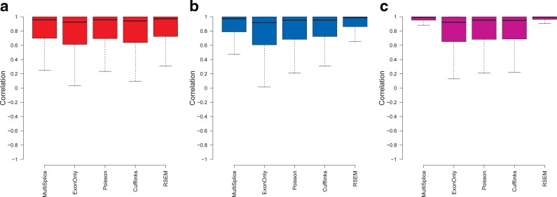
As shown in Figure 4, the performance of MultiSplice, RSEM, and ExonOnly method improves as the read-length increases. Accuracy of the Poisson model does not change much with varying read lengths. It is surprising to see that Cufflinks achieves better correlation with 100-bp single-end reads than both 2x50-bp paired-end reads and 50-bp single-end reads. This is probably because the transcript fragment inference from paired-end reads may not be accurate for Cufflinks. Both MultiSplice and RSEM show higher median correlation and lower variance compared with other methods under different read lengths, which indicates that MultiSplice and RSEM are capable of leveraging longer reads for more accurate estimation as RNA-seq technologies improve.

FIG. 4.

Boxplots of the correlation between estimated transcript proportions and the ground truth under varying read length. (a), (b), and (c) correspond to the estimation results on 40M 50-bp single-end reads, 40M 100-bp single-end reads, and 40M 2x50-bp paired-end reads, respectively.

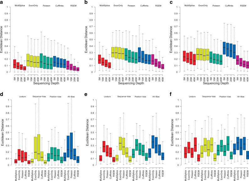
Varying sampling depth. Next we evaluate how the sequencing depth may affect the accuracy of transcript abundance estimation. Four groups of 2x50-bp paired-end synthetic data were generated on the whole human transcriptome with increasing number of reads: 5 million, 10 million, 20 million, and 40 million. Since the exonic regions of different genes may overlap, we quantify isoforms within a genomic locus (Trapnell et al., 2010); 13,364 genomic loci with multiple isoforms are selected for analysis. The loci were divided into three subsets: (1) 12,413 loci to which identifiability holds for all methods; (2) 498 loci to which identifiability holds for MultiSplice; and (3) 453 loci to which identifiability does not hold for all methods.

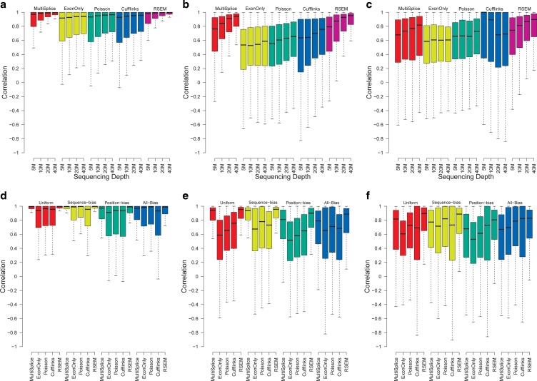
For each subplot in Figure 5a–c, the estimation accuracy for all methods generally improves as more reads are sampled. For the loci whose identifiability conditions are satisfied for all methods, the estimated transcript proportion is highly similar with the ground truth, with a median correlation close to 0.9 for all methods. In the second category, when the genes are still identifiable with MultiSplice, the estimation accuracy of MultiSplice and RSEM remain high, with a median correlation above 0.8 while others slip below 0.7. For the category when identifiability is not satisfied for all methods, the estimation accuracy is degraded even more. However, MultiSplice still consistently gives better estimation results indicating that the inclusion of MultiSplice features make transcript quantification more stable than other methods. Cufflinks demonstrated the worst performance in this category with largest variance as shown in Figure 9c in the Appendix section, mainly because the unidentifiability conditions make it difficult to assign these reads to a transcript. Instead, it throws out most of the multi-mapped reads. Apparently, increasing sampling depth cannot alleviate the issue of unidentifiability.

FIG. 5.

Boxplots of the correlation between estimated transcript proportions and the ground truth under varying number of sampled reads: 5M, 10M, 20M, and 40M over a total of 13,364 genomic loci with more than one isoforms. (a), (b), and (c) correspond to the loci set that is identifiable with basic exon structure, identifiable with additional MultiSplice features, and unidentifiable, respectively. (d–f) Boxplots of the correlation between estimated transcript proportions and the ground truth under four circumstances: uniform sampling, sampling with positional bias only, with sequence bias only, and with all bias. Panels (d), (e), and (f) correspond to the loci set that is identifiable with basic exon structure, identifiable with additional MultiSplice features, and unidentifiable, respectively.

FIG. 9.

Boxplots of the Euclidean distance between estimated transcript proportions and the ground truth under varying number of sampled reads: 5M, 10M, 20M, and 40M over a total of 13,364 genomic loci with more than one isoforms. Panels (a), (b), and (c) correspond to the loci set that is identifiable with basic exon structure, identifiable with additional MultiSplice features, and unidentifiable, respectively. (d—f) Boxplots of the Euclidean distance between estimated transcript proportions and the ground truth under four circumstances: uniform sampling, sampling with positional bias only, with sequence bias only, and with all bias. Panels (d), (e) and (f) correspond to the loci set that is identifiable with basic exon structure, identifiable with additional MultiSplice features, and unidentifiable, respectively.

Bias correction. To study the effect of the bias correction, we have simulated data with uniform sampling, sampling with only positional bias, sampling with only sequence bias, and sampling with the combined positional and sequence bias. Here, we set the slope of the position-specific bias k to 2 with 40 million 2x50-bp paired-end reads sampled from the whole transcriptome for each case. All the approaches achieve the best results when the sampling process is uniform. As positional or sequence bias is introduced, their performance tapers down. The presence of both positional and sequence biases has the largest impact in all methods. Meanwhile, because MultiSplice and Cufflinks correct both sequence and positional bias, and RSEM could adjust positional bias, these three methods are more robust and outperform the ExonOnly and the Poisson methods.

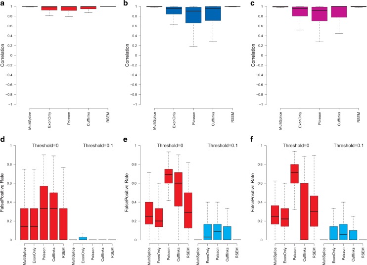
Inference of expressed transcripts. Quantification of mRNAs usually relies on a set of candidate transcript structures as input. It is unknown in a priori whether each transcript is present in a sample or not. Therefore, accurate quantification methods should be able to infer the transcripts that are expressed as well as those that are not. To assess the capability of the various methods to infer expressed transcripts, we generated 40 million simulated 2x50-bp paired-end reads from human genes with at least three transcripts. We randomly chose two transcripts from one gene and simulated reads only from these transcripts. The remaining transcripts were not sampled. We used the false-positive rate to measure the accuracy of the inference. Nonexpressed transcripts that were estimated with a positive abundance above a given threshold were counted as the false positives. As shown in Figure 6a–c, MultiSplice and RSEM demonstrated best estimation accuracy and further more MultiSplice demonstrated the lower false-positive rate in the identification of dominant transcripts in Figure 6d–f. Poisson and Cufflinks tended to assign positive expression to every transcript including those that are not expressed. MultiSplice, in general, outperformed the others in identifying the correct set of expressed transcripts.

FIG. 6.

Boxplots of the correlation between estimated transcript proportions and the ground truth. Panels (a), (b), and (c) correspond to the loci set that is identifiable with the basic exon structure, identifiable with additional MultiSplice features, and unidentifiable, respectively. (d–f) Comparison of false-positive rates in the inference of the expressed transcripts. Thresholds represent the minimum fraction of a transcript that is considered expressed. Panels (d), (e) and (f) correspond to the loci set that is identifiable with the basic exon structure, identifiable with additional MultiSplice features, and unidentifiable, respectively.

6.3. Real human RNA-seq experiment

We applied the set of transcript quantification methods to a dataset that was originally used by Singh et al. (2011) to study differential transcription. In this study, two groups of RNA-seq datasets were generated from SUM-102 and MCF-7, two breast cancer cell lines. Each group contains four samples as technical replicates. The RNA-seq data were generated from Illumina HISEQ2000. Each sample had approximately 80 million 100-bp single-end reads. About 60 million reads can be aligned to the reference genome by MapSplice. The UCSC human hg19 annotated transcripts were fed into each software for transcript quantification.

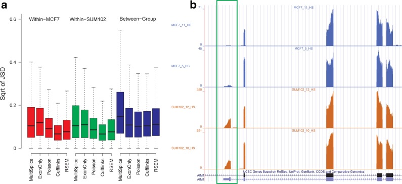
Since ground-truth expression profiles do not exist for the real datasets, we investigated whether the different methods provided a consistent estimation within samples of technical replicates, which only vary by random sampling. In contrast, a significant number of genes between MCF-7 and SUM-102 were expected to be differentially expressed (Singh et al., 2011). To evaluate this, we computed Jensen-Shannon divergence (JSD), used in Cuffdiff (Trapnell et al., 2010) to measure the dissimilarity between two samples and calculated the within-group and between-group differences. As detailed in Figure 7a, MultiSplice, Cufflinks, and RSEM had smaller average within-group difference than the average between-group difference, while the other two methods do not show clear difference. MultiSplice demonstrated higher between-group difference than both Cufflinks and RSEM, but also had relatively higher within-group differences as well. Most of these, however, were well below a JSD of 0.2 and considered to be insignificant. A closer look at a number of cases showed that occasionally MultiSplice and Cufflinks may overestimate or underestimate the between-group difference respectively. Figure 7b shows a gene where Cufflinks underestimated the difference between the two groups. (The complete figure with eight samples can be found in appendix Figure 11a.) The second isoform of the gene AIM1 has a unique first exon (chr6:106989461-106989496). Clear difference in the read coverage on this exon can be observed between the two groups, indicating strong differential levels of expression (i.e., the second isoform is barely expressed in MCF-7 while almost comparable to the first isoform in SUM-102 cells). The between-group square root of JSD is 0.21 by Cufflinks, lower than 0.39 by RSEM, and much lower than 0.50 by MultiSplice.

FIG. 7.

(a) Boxplots of the within-MCF-7, within-SUM-102, and between-group square root of JSD of all genes for all methods. (b) A case where Cufflinks underestimated the difference between the two groups. The second isoform of Gene AIM1 has a unique first exon, whose read coverage differs significantly between the two groups. A detailed plot with all eight samples can be found in Appendix Figure 11a.

FIG. 11.

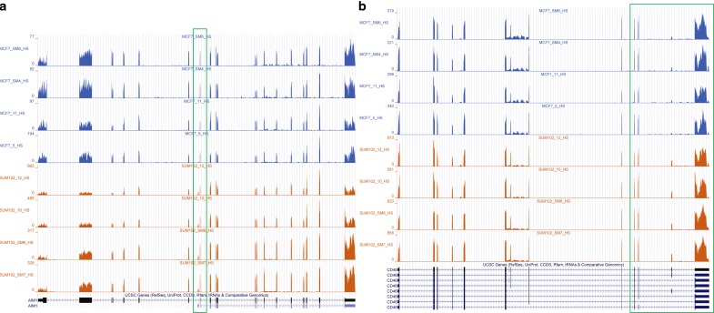
The coverage plot of Gene AIM1 in all eight breast-cancer cell-line samples. Please note the first exon of the second isoform is barely expressed MCF-7, but its expression significantly increased in the SUM-102 samples. (b) The coverage plot of Gene CD46. The exon-skipping event on the 13th exon has been confirmed by qRT-PCR.

The exon-skipping event found in gene CD46 is also differentially expressed (appendix Fig. 11b). The estimation of transcript quantification with MultiSplice was consistent with the observation in the qRT-PCR data showing that steady state levels of transcripts with the skipped exon were present in amounts more than two-fold higher expression in SUM-102 than in MCF-7 cells. An additional example can be found in the Appendix section.

Computational performance. We also compared the running time and memory usage of the proposed method with Cufflinks and RSEM. In order to make a fair comparison, we only measured the computational performance of transcript quantification for each software. One sample with 76 million reads from MCF-7 was used for analysis. The reads are aligned to the reference transcript set by Bowtie (Langmead et al., 2009) for RSEM and to the reference genome by MapSplice (Wang et al., 2010) for MultiSplice and Cufflinks. The results presented here were run on Intel Xeon X5650 (Westmere) 12-core 2.66 GHz Linux server with 32GB of RAM and single-thread enabled. Table 1 summarizes the comparison results of MultiSplice, Cufflinks, and RSEM.

Table 1.

Computational Performance Comparison

Method type	MultiSplice	Cufflinks	RSEM
Quantification time	40 min	74 min	23 h
Memory usage	<1G	2G	7G

7. Conclusion

In this article, we propose a general linear framework for the accurate quantification of alternative transcript isoforms with RNA-seq data. We introduce a set of new structural features, namely MultiSplice, to ameliorate the issue of identifiability. With MultiSplice features, 98% of UCSC gene transcript models in humans and mice become identifiable with 500-bp reads (or paired-end reads with 500-bp transcript fragments), an 8% increase from 50 bp. Therefore, longer reads or paired-end reads with longer insert sizes rather than further increases in sequencing depths can be crucial for the accurate quantification of mRNA isoforms with complex alternative transcription, even though a majority of the genes have relatively simple transcript variants. The results also demonstrate the robustness of the MultiSplice method under various sampling biases, consistently outperforming three other methods: Cufflinks, Poisson, and ExonOnly, and comparable to RSEM. The application of our approach to real RNA-seq datasets for transcriptional profiling successfully identified a number of isoforms whose proportion changes differed significantly between two distinct breast-cancer cell lines. In the near future, we will continue to experiment our algorithms with more complex gene models, including those from Ensembl database and those transcripts that are directly assembled from RNA-seq.

8. Appendix

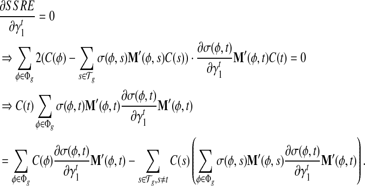
8.1. Iterative-minimization algorithm

In Section 5, we use an iterative-minimization strategy to search for a set of bias coefficients 's and 's for every transcript that better fit the RNA-seq sample than the uniform sampling model. We initiate the iterations with the transcript coverage C(t)'s solved from the uniform sampling model and the bias coefficients and . In each iteration, for transcript t we set:

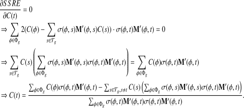σ(φ,t) is the only function related to γ^t₁ and γ^t₀.

Similarly,

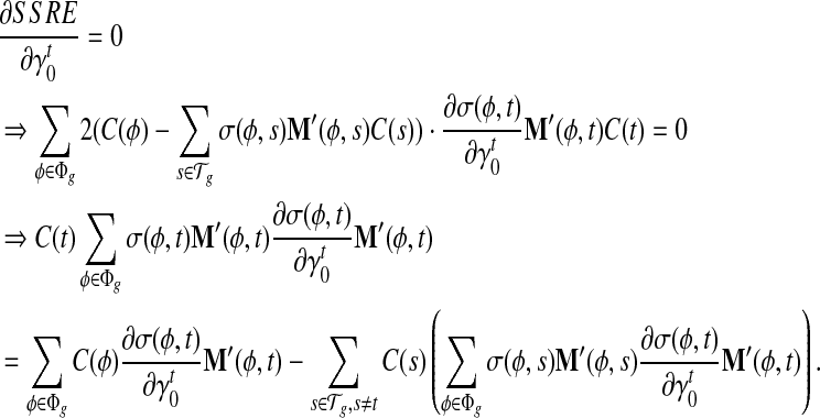Because σ(φ, t) is a linear combination of and , and hence is also the linear combination of and . Then we can directly calculate and .

FIG. 8.

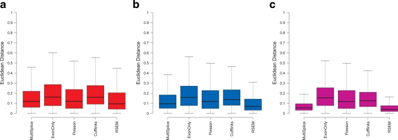
Boxplots of the Euclidean distance between estimated transcript proportions and the ground truth under varying read length Panels (a), (b), and (c) correspond to the estimation results on 40M 50-bp single-end reads, 40M 100-bp single-end reads, and 40M 2x50-bp paired-end reads, respectively.

FIG. 10.

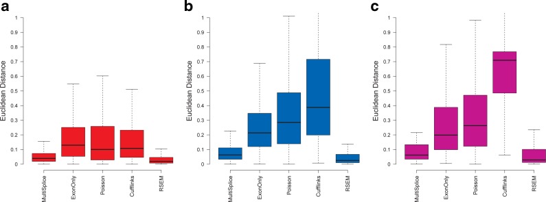
Boxplots of the Euclidean distance between estimated transcript proportions and the ground truth for inference of dominant transcripts. Panels (a), (b) and (c) correspond to the loci set that is identifiable with the basic exon structure, identifiable with additional MultiSplice features, and unidentifiable, respectively.

FIG. 12.

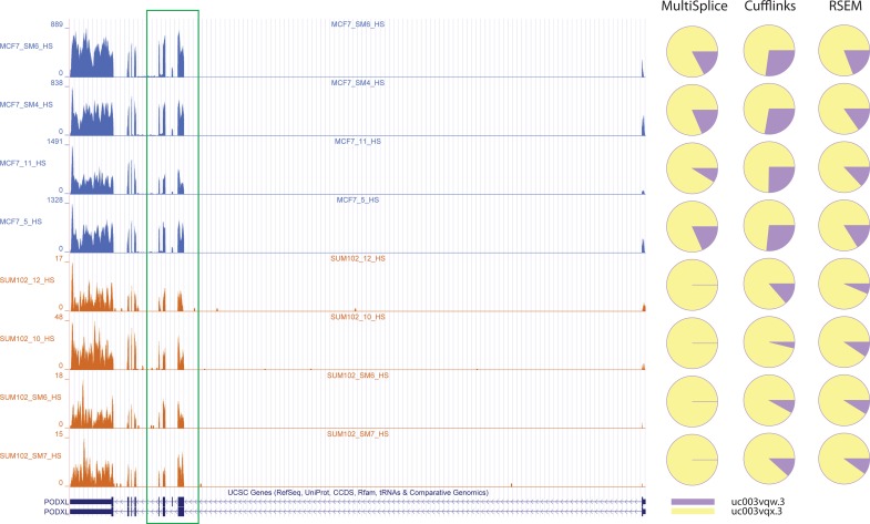
One real gene example for which MultiSplice inferred the expressed transcript while RSEM and Cufflinks failed to do so. The left figure shows the coverage plot of Gene PODXL in all eight breast-cancer cell-line samples. The between-group square root of JSD is 0.290611 by MultiSplice, 0.195271 by Cufflinks, and 0.094207 by RSEM. The exon-skipping event on the seventh (chr7: 131194995-131195090) are differentially expressed between two cell lines. The coverage plot indicates the first isoform is not expressed in SUM-102. The right part shows pie charts of estimated relative expression of the annotated two isoforms for three methods in all eight samples. Except MultiSplice, both Cufflinks and RSEM assign positive expression to the first isoform in SUM-102.

Acknowledgments

We thank the referees for their insightful comments. We thank Christian F. Orellana for running Cufflinks on real datasets. We thank Dr. Charles Perou for the RNA-seq samples from the MCF-7 and SUM-102 cell lines. Funding: This work was supported by The National Science Foundation (CAREER award grant number 1054631 to J.L.); the National Science Foundation (ABI/EF grant number 0850237 to J.L. and J.F.P.), and National Institutes of Health (grant number P20RR016481 to J.L.). Additional support was provided by the National Institutes of Health: NCI TCGA (grant number CA143848 to Charles Perou) and an Alfred P. Sloan Foundation fellowship (to D.Y.C.).

Author Disclosure Statement

The authors declare that no competing financial interests exist.

References

- Bejerano G. Algorithms for variable length Markov chain modeling. Bioinformatics. 2004;20:788–789. doi: 10.1093/bioinformatics/btg489. [DOI] [PubMed] [Google Scholar]
- Bohnert R. Rätsch G. rQuant.web: a tool for RNA-Seq-based transcript quantitation. Nucleic Acids Res. 2010;38(Suppl 2):W348–W351. doi: 10.1093/nar/gkq448. [DOI] [PMC free article] [PubMed] [Google Scholar]
- Brosseau J.P. Lucier J.F. Lapointe E., et al. High-throughput quantification of splicing isoforms. RNA. 2010;16:442–449. doi: 10.1261/rna.1877010. [DOI] [PMC free article] [PubMed] [Google Scholar]
- Feng J. Li W. Jiang T. Inference of isoforms from short sequence reads. J. Comput. Biol. 2010;18:305–21. doi: 10.1089/cmb.2010.0243. [DOI] [PMC free article] [PubMed] [Google Scholar]
- Flicek P. Amode M.R. Barrell D., et al. Ensembl 2012. Nucleic Acids Res. 2012;40:D84–D90. doi: 10.1093/nar/gkr991. [DOI] [PMC free article] [PubMed] [Google Scholar]
- Guttman M. Garber M. Levin J.Z., et al. Ab initio reconstruction of cell type-specific transcriptomes in mouse reveals the conserved multi-exonic structure of lincRNAs. Nat. Biotechnol. 2010;28:503–510. doi: 10.1038/nbt.1633. [DOI] [PMC free article] [PubMed] [Google Scholar]
- Horn R.A. Johnson C.R. Matrix analysis. Cambridge University Press; Cambridge, United Kingdom: 1990. [Google Scholar]
- Hu Y. Wang K. He X., et al. A probabilistic framework for aligning paired-end RNA-seq data. Bioinformatics. 2010;26:1950–1957. doi: 10.1093/bioinformatics/btq336. [DOI] [PMC free article] [PubMed] [Google Scholar]
- Jiang H. Wong W.H. Statistical inferences for isoform expression in RNA-Seq. Bioinformatics. 2009;25:1026–1032. doi: 10.1093/bioinformatics/btp113. [DOI] [PMC free article] [PubMed] [Google Scholar]
- Kozarewa I. Ning Z. Quail M.A., et al. Amplification-free Illumina sequencing-library preparation facilitates improved mapping and assembly of (G+C)-biased genomes. Nat. Methods. 2009;6:291–5. doi: 10.1038/nmeth.1311. [DOI] [PMC free article] [PubMed] [Google Scholar]
- Kristi L.F. Dou Y. Bianca J.L., et al. The architecture of pre-mRNAs affects mechanisms of splice-site pairing. Proc. Natl. Acad. Sci. U.S.A. 2005;102:16176–16181. doi: 10.1073/pnas.0508489102. [DOI] [PMC free article] [PubMed] [Google Scholar]
- Lacroix V. Sammeth M. Guigo R., et al. Exact transcriptome reconstruction from short sequence reads; Proceedings of the 8th International Workshop on Algorithms in Bioinformatics.2008. [Google Scholar]
- Langmead B. Trapnell C. Pop M., et al. Ultrafast and memory-efficient alignment of short DNA sequences to the human genome. Genome Biol. 2009;10:R15. doi: 10.1186/gb-2009-10-3-r25. [DOI] [PMC free article] [PubMed] [Google Scholar]
- Li B. Dewey C.N. RSEM: accurate transcript quantification from RNA-Seq data with or without a reference genome. BMC Bioinf. 2011;12:323. doi: 10.1186/1471-2105-12-323. [DOI] [PMC free article] [PubMed] [Google Scholar]
- Li B. Ruotti V. Stewart R.M., et al. RNA-Seq gene expression estimation with read mapping uncertainty. Bioinformatics. 2010;26:493–500. doi: 10.1093/bioinformatics/btp692. [DOI] [PMC free article] [PubMed] [Google Scholar]
- Li J. Jiang H. Wong W.H. Modeling non-uniformity in short-read rates in RNA-Seq data. Genome Biol. 2010;11:R50. doi: 10.1186/gb-2010-11-5-r50. [DOI] [PMC free article] [PubMed] [Google Scholar]
- Li W. Feng J. Jiang T. IsoLasso: A LASSO Regression Approach to RNA-Seq Based Transcriptome Assembly. RECOMB. 20112011:168–188. doi: 10.1089/cmb.2011.0171. LNBI 6577. [DOI] [PMC free article] [PubMed] [Google Scholar]
- Lia J. Jiang C. Browna J.B., et al. Sparse linear modeling of next-generation mRNA sequencing (RNA-Seq) data for isoform discovery and abundance estimation. Proc. Natl. Acad. Sci. U.S.A. 2011 doi: 10.1073/pnas.1113972108. [DOI] [PMC free article] [PubMed] [Google Scholar]
- Nicolae M. Mangul S. Mandoiu I.I., et al. Estimation of alternative splicing isoform frequencies from RNA-Seq data. Algorithms for Molecular Biology. 2011;6:9. doi: 10.1186/1748-7188-6-9. [DOI] [PMC free article] [PubMed] [Google Scholar]
- Olejniczak M. Galka P. Krzyzosiak W.J. Sequence-non-specific effects of RNA interference triggers and microRNA regulators. Nucleic Acids Res. 2010;38:1–16. doi: 10.1093/nar/gkp829. [DOI] [PMC free article] [PubMed] [Google Scholar]
- Pan Q. Shai O. Lee L.J., et al. Deep surveying of alternative splicing complexity in the human transcriptome by high-throughput sequencing. Nat. Genet. 2008;40:1413–1415. doi: 10.1038/ng.259. [DOI] [PubMed] [Google Scholar]
- Pruitt K.D. Tatusova T. Maglott D.R. NCBI reference sequences (RefSeq): a curated non-redundant sequence database of genomes, transcripts and proteins. Nucleic Acids Res. 2007;35:D61–D65. doi: 10.1093/nar/gkl842. [DOI] [PMC free article] [PubMed] [Google Scholar]
- Richard H. Schulz M.H. Sultan M., et al. Prediction of alternative isoforms from exon expression levels in RNA-Seq experiments. Nucleic Acids Res. 2010;38:e112. doi: 10.1093/nar/gkq041. [DOI] [PMC free article] [PubMed] [Google Scholar]
- Roberts A. Trapnell C. Donaghey J., et al. Improving RNA-Seq expression estimates by correcting for fragment bias. Genome Biol. 2011;12:R22. doi: 10.1186/gb-2011-12-3-r22. [DOI] [PMC free article] [PubMed] [Google Scholar]
- Russell S. Norvig P. Artificial Intelligence: A Modern Approach. Prentice Hall; Saddle River, NJ: 2003. [Google Scholar]
- Singh D. Orellana C.F. Hu Y., et al. FDM: A graph-based statistical method to detect differential transcription using RNA-seq data. Bioinformatics. 2011;27:2633–40. doi: 10.1093/bioinformatics/btr458. [DOI] [PMC free article] [PubMed] [Google Scholar]
- Tibshirani R. Regression shrinkage and selection via the lasso. J. R. Stat. Soc. 1996;58:267–288. [Google Scholar]
- Trapnell C. Williams B.A. Pertea P., et al. Transcript assembly and quantification by RNA-Seq reveals unannotated transcripts and isoform switching during cell differentiation. Nat. Biotechnol. 2010;28:511–515. doi: 10.1038/nbt.1621. [DOI] [PMC free article] [PubMed] [Google Scholar]
- Turro E.S.S. Concalves A. Haplotype and isoform specific expression estimation using multi-mapping RNA-seq reads. Genome Biol. 2011;12:R13. doi: 10.1186/gb-2011-12-2-r13. [DOI] [PMC free article] [PubMed] [Google Scholar]
- Srivastava S. Chen L. A two-parameter generalized Poisson model to improve the analysis of RNA-seq data. Nucleic Acids Res. 2010;38:e170. doi: 10.1093/nar/gkq670. [DOI] [PMC free article] [PubMed] [Google Scholar]
- Wang E.T. Sandberg R. Luo S., et al. Alternative isoform regulation in human tissue transcriptomes. Nature. 2008;456:470–476. doi: 10.1038/nature07509. [DOI] [PMC free article] [PubMed] [Google Scholar]
- Wang K. Singh D. Zeng Z., et al. MapSplice: Accurate mapping of RNA-seq reads for splice junction discovery. Nucleic Acids Res. 2010;38:178. doi: 10.1093/nar/gkq622. [DOI] [PMC free article] [PubMed] [Google Scholar]
- Wang Z. Gerstein M. Snyder M., et al. RNA-Seq: a revolutionary tool for transcriptomics. Nat. Rev. Genet. 2009;10:57–63. doi: 10.1038/nrg2484. [DOI] [PMC free article] [PubMed] [Google Scholar]
- Wu J. Akerman M. Sun S., et al. SpliceTrap: a method to quantify alternative splicing under single cellular conditions. Bioinformatics. 2011;27:3010–3016. doi: 10.1093/bioinformatics/btr508. [DOI] [PMC free article] [PubMed] [Google Scholar]
- Wu Z. Wang X. Zhang X. Using non-uniform read distribution models to improve isoform expression inference in RNA-Seq. Bioinformatics. 2011;27:502–508. doi: 10.1093/bioinformatics/btq696. [DOI] [PubMed] [Google Scholar]