Incorporating auxiliary information for improved prediction in high-dimensional datasets: an ensemble of shrinkage approaches

Abstract

With advancement in genomic technologies, it is common that two high-dimensional datasets are available, both measuring the same underlying biological phenomenon with different techniques. We consider predicting a continuous outcome Y using X, a set of p markers which is the best available measure of the underlying biological process. This same biological process may also be measured by W, coming from a prior technology but correlated with X. On a moderately sized sample, we have (Y,X,W), and on a larger sample we have (Y,W). We utilize the data on W to boost the prediction of Y by X. When p is large and the subsample containing X is small, this is a p>n situation. When p is small, this is akin to the classical measurement error problem; however, ours is not the typical goal of calibrating W for use in future studies. We propose to shrink the regression coefficients β of Y on X toward different targets that use information derived from W in the larger dataset. We compare these proposals with the classical ridge regression of Y on X, which does not use W. We also unify all of these methods as targeted ridge estimators. Finally, we propose a hybrid estimator which is a linear combination of multiple estimators of β. With an optimal choice of weights, the hybrid estimator balances efficiency and robustness in a data-adaptive way to theoretically yield a smaller prediction error than any of its constituents. The methods, including a fully Bayesian alternative, are evaluated via simulation studies. We also apply them to a gene-expression dataset. mRNA expression measured via quantitative real-time polymerase chain reaction is used to predict survival time in lung cancer patients, with auxiliary information from microarray technology available on a larger sample.

1. Introduction

As sequencing and array technologies change, multiple platforms can measure the same biological quantity of interest. Often investigators have measurements using an older technology on a large sample and those from a newer technology on a subset of this sample. We are interested in predicting an outcome using the newer measurements, which is a statistical problem of fitting a prediction model for Y |X, where Y is the outcome and X is the p-dimensional vector of biomarkers. One such model is a linear regression:

(1.1)

On n_A subjects, we have Y , X, and W, where W, also of length p, measures the same biomarkers as does X but with a prior technology. A model for W|X consistent with this motivating context is

(1.2)

Here I_p is the identity matrix and ψ, ν, and τ are scalars. For notational simplicity, we develop methods under the assumption β₀=ψ=0. Both quantities are estimated in our analyses.

The quantity n_A is of modest size, such that p>n_A. Additionally, n_B observations of Y and W are available. Assume p<n_B. Denote subsamples A and B (each assumed to be from the same population) by (y_A,x_A,w_A) and (y_B,w_B), respectively. Using this notation, x_B, the set of X's from subsample B, is missing. Figure1 gives a schematic representation. x_A is also standardized, i.e. if x_ij is from the ith row and jth column, and , j=1,…,p.

Fig. 1.

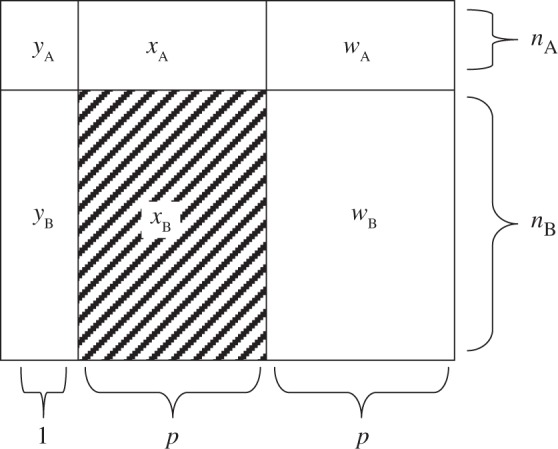
The schematic representation of the prediction problem: (y_A,x_A,w_A) constitutes subsample A, of size n_A, and (y_B,w_B) constitutes subsample B, of size n_B. The covariates represented by x_B are considered missing. The quantity W is an error/prone noisy version of X. The goal is to utilize the data on W to boost the prediction of Y by X.

The goal is a prediction model for Y_new|X_new for a new subject: . Predictive performance of is measured by mean squared prediction error (MSPE), defined as

(1.3)

where indicates the trace operator, and the expectation is over Y_new,X_new,y_A,y_B|x_A,w_A,w_B. We consider two questions: (i) How can the auxiliary information in subsample B be used in the prediction of Y |X? (ii) When does using such information lead to an improved MSPE?

A simple approach, which ignores subsample B, is ordinary least squares of y_A on x_A, i.e. . However, (x^⊤_Ax_A)⁻¹ does not exist for p>n_A. Even for p≤n_A, multicollinearity of the covariates may lead to variance inflation and numerical instability. Ridge regression (ridg) (Hoerl and Kennard, 1970) can ameliorate these issues by shrinking coefficients toward zero, i.e. . This can be viewed from a Bayesian perspective: given a normal prior on β with mean 0_p and precision σ⁻²λI_p, the ridg coefficients are the posterior mode for a given λ. Hoerl and Kennard showed that there exists λ>0 which decreases the mean squared error of , , compared with λ=0. ridg penalizes the L₂ norm; other methods exist which constrain the L_d norm for some d (e.g. Frank and Friedman, 1993. In contrast to variable selection procedures, which might use an L₁ penalty, our goal is using auxiliary information to boost prediction, and so we restrict attention to ridge-type estimators.

Dempster and others (1977) evaluate 57 variants of shrinkage estimators and argue for ridg. Draper and van Nostrand (1979) are critical of ridg because of difficulties in choosing the parameter λ. However, Craven and Wahba (1979) and Li (1986) demonstrate the asymptotic optimality of the generalized cross-validation (GCV) function in selecting λ. Simulation studies Gelfand, 1986; Frank and Friedman, 1993 demonstrate good prediction properties of ridg for many choices of β. Rao (1975) generalizes ridg to allow for different levels of shrinkage between each coefficient. Swindel (1976) proposes ridge estimators that take into account prior information, changing the direction of shrinkage. Casella (1980) and Maruyama and Strawderman (2005) propose variants of ridge estimators with minimax properties. Sclove (1968) adapts the shrinkage estimator of James and Stein (1961) (JS) which, for p>3, uniformly beats the maximum likelihood estimate (MLE) of β in terms of MSE. Gruber (1998) offers a unified treatment of different kinds of JS and ridge estimators from frequentist and Bayesian points of view.

By incorporating subsample B, this may be viewed as a problem of combining multiple estimators. George (1986) proposes JS estimators that shrink toward multiple targets. Green and Strawderman (1991) consider a targeted JS estimator: an unbiased estimator is shrunk toward a biased but more efficient estimator so as to minimize MSE under certain assumptions. LeBlanc and Tibshirani (1996) propose linear combinations of regression coefficients to improve prediction error. This bias and variance trade-off in combining estimators has been used in recent genetic studies((Chen and others, 2009)).

For p<n_A, the problem closely resembles that of measurement error (ME) in the covariates, W being an error-prone version of X. Fuller (1987) and Carroll and others (2006) review ME methods for unbiased and efficient inference on β. In linear regression, using W instead of X gives biased estimates of β. However, this substitution is typically not problematic for predicting Y_new with . Our prediction model of interest being Y given X, this bias in from using W instead of X does bias away from Y_new. Regression calibration, which fills in each missing X with its conditional expectation given W, may provide unbiased estimates of β and therefore Y_new. In contrast, although the substitution of X by W gives biased estimates of β, it may reduce the variance of estimates of β relative to regression calibration (Buzas and others, 2005) and consequently reduce MSPE. Even for p<n_A, then, it is not evident that the regression calibration algorithm is best for making predictions with .

This paper makes several new contributions. We consider an important but non-standard prediction problem which has not yet received a rigorous mathematical treatment. We introduce a class of targeted ridge (TR) estimators, borrowing ideas from the shrinkage and regression calibration literature. We also consider combining an ensemble of TR estimators, as in Green and Strawderman (1991). In contrast to minimizing MSE, we determine the shrinkage weights adaptively so as to minimize MSPE. Interestingly, one is able to combine two or more biased estimators of β for better prediction than any individual estimator. This result applies to a linear combination of any set of estimates of β. We evaluate all of these estimators via simulation studies and a data analysis.

The rest of the paper is organized as follows. In Section2, we unify ridg and regression calibration methods under a class of TR estimators. In Section3, we propose hybrid estimators that achieve superior prediction by data-adaptively combining multiple estimators. Section4 gives a fully Bayesian alternative and Section5 presents a simulation study. Section6 applies the methods: survival time (Y) in lung cancer patients is predicted with quantitative real-time polymerase chain reaction (qRT-PCR) data (X), aided by microarray data (W) from a larger sample. Section7 concludes with a discussion. Analytical details are in supplementary material available at Biostatistics online.

2. Targeted shrinkage

For p>n_A, ordinary least squares using subsample A is not applicable. In fact, when X_new is not in the column space of x_A, no unbiased estimate of X^⊤_newβ using only subsample A exists (Rao, 1945). A biased alternative is ridge regression (Hoerl and Kennard, 1970,

(2.1)

ridg is equivalent to adding λ to each eigenvalue of x^⊤_Ax_A, thus allowing the matrix inversion. The coefficient estimates are shrunk to zero, more so for larger values of λ. That the ridge estimator is applicable for p>n_A is crucial in our setting. Shrinkage estimators from Sclove (1968) and Casella (1980) make use of unbiased estimators of β and hence are not directly applicable for p>n_A situations.

For ridge regression, Craven and Wahba (1979) proposed to select λ using the GCV function, choosing the λ that minimizes

(2.2)

where Θ is an arbitrary p×p positive semi-definite (PSD) matrix. Rao (1975) suggested that any PSD matrix Ω⁻¹_β can replace I_p in (2.1). Swindel (1976) proposed to shrink toward a non-null vector γ_β. From the Bayesian perspective, these replace the prior precision σ⁻²λI_p in ridg with σ⁻²λΩ⁻¹_β and the prior mean 0_p with γ_β. The posterior mode is

(2.3)

(2.4)

Gruber (1998, p.241) calls this a generalized ridge estimator. Because “generalized ridge” has been used for several distinct methods in the shrinkage literature, we instead call this a TR estimator, referring to shrinkage toward a target γ_β. The estimator in (2.4) gives the three terms which determine the general class of TR estimators. As we shall see, different estimators, we propose either implicitly or explicitly specify values for . In particular, ridg is a TR estimator: .

As stated in (1.3), . Thus, we calculate the MSPE of a TR estimator from its bias and variance, taking expectations over the response distribution y_A,y_B|x_A,w_A,w_B:

(2.5)

(2.6)

These expressions assume that λ and Ω⁻¹_β are fixed with respect to y_A,y_B|x_A,w_A,w_B but allow γ_β to be data-dependent. A TR estimator may use a true prior, as in ridg, in which case γ_β is fixed.

We now propose several other TR estimators. If x_B were observed, logical selections of γ_β and Ω⁻¹_β would be and x^⊤_Bx_B, respectively, with λ=1, giving the estimator . In the absence of x_B, the naïve inclination is to regress y_B on w_B and use and w^⊤_Bw_B as γ_β and Ω⁻¹_β, that is, use w_B itself as an imputation for x_B. We first consider approaches that derive a replacement for the missing x_B which may be better than w_B. This is obtained by modeling W|X based on the relationship observed in subsample A and thereby inducing data-driven values of γ_β and Ω⁻¹_β. From the ME perspective, this is regression calibration. These TR estimators fix λ=1 (data-adaptive estimation of λ may be done using, e.g. a GCV criterion).

Structural regression calibration (src): A distribution on X and the ME model for W|X imply a value of [X|W]. src fills in the missing x_B with its conditional expectation given w_B. Assuming that X is normal, say N_p{μ_X,Σ_X}, implies that X|W is also normal. Let . From properties of the conditional distribution of X|W,

(2.7)

(2.8)

We suppress the dependence on θ of x^src_B(θ), M(θ), and V(θ) hereafter. This is a precision-weighted average of and (1/ν)w_B. Using (2.4), define , with and . In the ME literature, src is the standard “Regression Calibration” approach. We append “Structural” (Carroll and others, 2006, p.25), referring to a distributional assumption about X, to distinguish from its “Functional” alternative, which does not assume this, proposed as follows.

Functional regression calibration (frc): Solving (1.2), W=νX+τξ, for X gives X=(1/ν)W−(τ/ν)ξ. Another natural estimate of x_B, and consequently a corresponding γ_β and Ω⁻¹_β, is therefore

(2.9)

This gives a TR estimate defined as . This imputation for x_B is a scaled version of a substitution of w_B for x_B, to which frc is equivalent when ν=1, i.e. under the classical ME model. In supplementary material available at Biostatistics online (Appendix A), we conduct extensive analyses which suggest that frc is preferred over src in terms of MSPE as any of β^⊤β, σ², or τ/ν increase.

The first rows of Table1 summarize choices of for ridg, frc, and src. Assuming that the ME is non-differential, i.e. [Y |X,W]=[Y |X], and μ_X=0_p, Table1 also gives γ_β and γ_β for frc and src. Because γ_βsrc=β, from (2.5), src provides unbiased estimates of β.

Table 1.

Key information for several TR estimators, conditioning on the true value of θ

Method	γβ	Ω−1β	λ=1?
ridg	0p	Ip	N
frc			Y
src			Y
Method	γβ	γβ
ridg	—	—
frc	Vβ	(σ2+κ)ν2(w⊤BwB)−1
src	β

κ=(τ²/ν²)β^⊤Vβ. . The “λ=1?” column indicates whether λ is fixed at 1 or tuned in a data-adaptive fashion using the general GCV function. The corresponding estimator is given by plugging into (2.4). The expectation and variance of γ_β, which are useful for calculating the MSPE of , are over y_A,y_B|x_A,w_A,w_B under the assumption [Y |X,W]=[Y |X].

Remark 2.1 —

One of the reviewers observed that, when γ_β and Ω⁻¹_β are based on historical data, the prior in the second expression of (2.3) is a power prior (Chen and Ibrahim, 2000), with λ controlling the contribution of the historical data to the posterior.

Remark 2.2 —

These approaches require estimating . One can regress {w_ij} on {x_ij} for i=1,…,n_A and j=1,…,p , to compute MLEs for ν and τ. If it is required that ν and τ be of a more general form than scalar-valued, the estimation procedure can be modified accordingly. The MLE for μ_X is , which will be 0_p if x_A is standardized. For p>n_A, the required inversion of is not possible. An alternative is the shrinkage estimator from Schäfer and Strimmer (2005): since x^⊤_Ax_A is standardized, it is simply , for η∈[0,1] chosen data-adaptively. We used the R package corpcor to choose η targeting a minimum MSE for .

Remark 2.3 —

The bias and variance outlined in Table1 condition on the true value of θ and are over and above any bias and variance coming from its estimation. In particular, estimating Σ_X may pose a challenge to src in the high-dimensional setting.

Remark 2.4 —

One other approach which we do not further explore is modifying frc or src to do adaptive, component-wise shrinkage on β: a TR estimator where Ω⁻¹_β is diagonal and λ is estimated. When λ is not fixed, the GCV approach may be used to choose an appropriate value of λ. The form of this modified GCV criterion is given later on in (3.2), in connection with the hybrid estimator.

3. Hybrid estimators

While a particular TR estimator may do well for a given set of factors, e.g. p, n_B, β, τ, none is likely to give a small prediction error under all settings. However, a hybrid estimator, that is, an adaptively combined set of multiple TR estimators, may yield this flexibility. Given m estimators, , and a vector ω={ω₁,ω₂,…,ω_m} such that , let . The vector ω determines the contribution from each ; a sensible choice for ω in our situation would be the one that minimizes (b(ω)). The following theorem compares the prediction error of the resulting optimal hybrid estimator, b(ω^opt), to that of its constituents. The result uses the following definition of the “mean cross-product prediction error” between and :

(3.1)

Theorem 3.1 —

Let be a hybrid estimator. (i) If has at least one positive eigenvalue for every , then there exists a unique vector ω^opt which minimizes (b(ω)) subject to . (ii) Further, let . If for some i≠j, then .

The proof is in supplementary material available at Biostatistics online (Appendix B). If the assumptions are satisfied, then, using prediction error as the criterion, b(ω^opt) will perform better than the best of its constituents. This phenomenon has been observed empirically by Breiman (1996) and LeBlanc and Tibshirani (1996). Fumera and Roli (2005) prove a slightly weaker result for ensembles of classifiers.

Now, (b(ω))=ω^⊤Pω, where P is the m×m matrix with the (ij)th element given by , which is just when i=j. The results from Theorem3.1 apply when P is known. In practice, however, P and therefore ω^opt must be estimated. Since P_ij is equivalently expressed as , one might use as an estimate, but this will be biased. A generalization of a result from Mallows (1973) in supplementary material available at Biostatistics online (Lemma B.3) gives that, on average, this underestimates P_ij by the amount σ²(ψ_i+ψ_j), where . Borrowing Mallows’ idea of adjusting by does not work when there is no good choice of . We propose as an alternative adapting the GCV approach:

(3.2)

where y^*_,ℓ=y_A−x_Aγ_β,ℓ. Because , this is a penalized version of its naïve counterpart. Lemma B.4 (see supplementary material available at Biostatistics online) provides further justification for this approach.

Note the dual use of the GCV function to calculate b(ω). First, for each ℓ, λ_ℓ is chosen, when required, to minimize . Then, fixing these choices of λ_ℓ, (3.2) is employed on the m(m+1)/2 pairwise combinations of components in b(ω) to estimate P. The particular hybrid estimator we evaluate has three components: . Following LeBlanc and Tibshirani (1996), in addition to the constraint , we enforce a non-negativity constraint on ω, which improves numerical results.

Remark 3.2 —

The key aspect that makes practical is that the sum is the quantity to minimize. Estimating either of the terms alone is difficult. Green and Strawderman (1991) propose a similar combination of two estimators which minimizes the MSE of b(ω). For their method, the estimation of ω^opt requires an unbiased and independent estimators and . In our case, because MSPE, not MSE, is of interest, we require neither unbiasedness nor independent estimators.

Remark 3.3 —

Although Theorem3.1 proves hyb has a smaller MSPE than any of its constituents when using the true optimal weights ω^opt, for a given dataset with estimated optimal weights , this uniform dominance may not hold. Numerical performance depends on how accurately (3.2) estimates P. As will be seen, with estimated weights still performs well across a spectrum of scenarios and closely adapts to the best of its constituents.

4. Bayesian ridge

As a comparison to our proposed TR methods, we consider a fully Bayesian ridge regression which iteratively samples x_B and all model parameters from their full conditional distributions. We now briefly describe the construction of this approach; most details are in supplementary material available at Biostatistics online (Appendix C). We assume the models given in (1.1) and (1.2), along with X∼N_p{μ_X,Σ_X}. Let denote the set of all parameters. The likelihood of a complete observation may be factorized as

(4.1)

Given the observed data, {y_A,x_A,w_A,y_B,w_B}, and ϕ, each row of x_B is independently multivariate Normal; the data augmentation step samples x_B from this distribution to complete the likelihood. With respect to prior specification, we assume that β is N_p{0_p,(σ²/λ)I_p} (making this a Bayesian ridge) and Σ⁻¹_X is Wishart with 3p degrees of freedom and scale , where is the diagonal part of the empirical covariance of x_A. From our numerical studies, this Wishart prior on Σ⁻¹_X ensures the convergence of the algorithm in spite of the large fraction of missing data, represented by x_B. For the remaining components, Jeffrey's priors were used, that is, β₀, , ψ, ν, , μ_X , and , each have flat priors. In summary,

(4.2)

The Gibbs steps (Appendix C of supplementary material available at Biostatistics online) sample ϕ from its full conditional distribution derived from the product of the complete data likelihood and the prior. After a burn-in of 2000 iterations, we stored 1000 posterior draws of ϕ. For the sake of comparison to the other methods, which yield a point estimate of β, we used the posterior mean of β, denoted as , for predicting future observations.

5. Simulation study

We next describe a small simulation study. We fixed n_A=50 and used n_Bisinv;{400,150}. The diagonal elements of Σ_X were set to unity, and the off-diagonals were ρ^{|j₁−j₂|}, ρ∈{0,0.75}. Using these parameters, x_A and x_B were drawn from N_p{0_p,Σ_X}. We considered both high- (p=99) and low (p=5) -dimensional models: . The coefficient of determination, R², was either 0.1 or 0.4. Thus, given β, Σ_X and R², σ was determined by solving β^⊤Σ_Xβ/(β^⊤Σ_Xβ+σ²)=R². The intercept β₀ was set to zero; y_A|x_A and y_B|x_B were drawn for each combination of β and σ from (1.1). This yielded 16 unique simulation settings: two choices each for p, n_B, ρ, and R². To draw the auxiliary data, we set ψ=0 and ν=1 and repeated each of the 16 settings using τ∈(0,2), drawing w_A|x_A and w_B|x_B from (1.2).

For ridg, src, frc, hyb, and hierbetas, we estimated MSPE by averaging the squared prediction error over 1000 new individuals. Figure2 plots this empirical MSPE averaged over 1000 replicates over τ. For reference, σ², the smallest achievable MSPE, is also given. Tables S2 and S3 in supplementary material available at Biostatistics online provide numeric values of the empirical MSPE over all settings. Note that, in practice, the analyst estimates β₀ in addition to β. Following the common prescription for ridge regression, we did not shrink β₀ but instead used a flat prior in each of the TR methods and hierbetas.

Fig. 2.

Empirical MSPE over τ for the simulation study described in Section5. Here p stands for the number of covariates, n_B is the size of subsample B, ρ is the first-order auto-regressive correlation coefficient for pairwise combinations of X, and R²=β^⊤Σ_Xβ/(β^⊤Σ_Xβ+σ²). The top strip varies between rows and the bottom strip varies between columns. In all cases, n_A=50, β₀=ψ=0, and ν=1. σ², plotted in black, is the smallest possible MSPE for any estimate of β.

Effect of τ: ridg is not affected by τ, as it does not use w_A or w_B. frc and src are equivalent when τ is very small, close to the complete data case. The MSPE of src always rises with τ; this increase is sharp when p=99. However, larger values of τ give favorable shrinkage in frc. When p=99, the τ for which frc is best is larger than zero; for p=5, the “optimal” τ is quite small, and the MSPE rises sharply with τ. For p=99, the MSPE of hyb and hierbetas is mostly invariant to τ, except for when ρ=0 and R²=0.4. When p=5, hyb does a better job of improving upon its constituents when τ is large.

Effect of n_B, p, ρ, R²: As is expected, larger values of n_B decrease the MSPE for all methods except ridg. Notably, hyb sometimes fares poorly compared with frc (see Remark3.3) when p=99, n_B=400, and ρ=0.75, but otherwise outperforms its constituents in the p=99 cases. src fares poorly when p=99. Overall, hierbetas is the best-performing method in terms of MSPE. The relative difference between all methods is small when p=5.

Appendix D in supplementary material available at Biostatistics online additionally looks at MSE and investigates several violations to the modeling assumptions in this study. While hierbetas continues to predict very well, another important result is that hyb, which is less expensive computationally, is still flexible: under a variety of model settings and violations, hyb is able to efficiently adhere to the best-performing of its constituents.

6. Predicting survival time from gene expression measurements

We consider whether gene expression measurements offer information for predicting survival time in patients with lung cancer. Expression data may be collected using microarray technology, which assays the mRNA transcripts of thousands of genes. Alternatively, qRT-PCR amplifies gene expression in a targeted region of DNA so as to precisely measure it. Expression is measured as the number of doublings until a threshold is reached. It is both clinically practical to measure on a new tissue specimen, not requiring the specialized laboratory facilities of microarrays, and typically considered a more precise measurement of gene expression than microarrays.

Our dataset comes from Chen and others (2011), who selected p=91 high-correlating genes representing a broad spectrum of biological functions upon which to build a predictive model. Expression on the log-scale using Affymetrix (a microarray technology, W) was measured on 439 tumor samples, and qRT-PCR measurements (X) were collected on 47 of these tumors. The individual correlations between the qRT-PCR and Affymetrix measurements from the 47 tumors are greater than 0.5 across the 91 genes. Clinical covariates, age, gender, and stage of cancer (I–III), are also available. Because qRT-PCR is the clinically applicable measurement for future observations, the goal is a qRT-PCR + clinical covariate model for predicting log-survival time after surgery (Y). An independent cohort of 101 tumors with qRT-PCR measurements and clinical covariates is available for validation.

Eleven measurements in the qRT-PCR-only data, out of 47×91=4277 total, or 0.26 % were missing; in order to use all observations, these values were imputed using chained equations and thereafter assumed known. Additionally, four tumors, three in the Affymetrix-only sample and one in the validation sample, had event times less than 1 month after surgery, and these were removed before analysis. Thus, n_A=47, n_B=389, and the validation data contain 100 observations.

Because our methodology was developed for continuous outcomes, censoring necessitated some preprocessing of the data. We first imputed each censored log-survival time from a linear model of the clinical covariates, conditional upon the censoring time. This model was fit to the training data but was applied to censored survival times in both the training and validation data. Given completed log-survival times, we refit this same model and calculated residuals from both the training and validation data. These residuals were considered as outcomes, and the question is whether any additional variation in the residuals is explained by gene expression.

Figure S4 (see supplementary material available at Biostatistics online) presents the 91 LOESS curves comparing measurements from the 47 tumors using Affymetrix (w_A) to qRT-PCR (x_A) after standardization. Based on this, we used a gene-specific ME model: w_ij=ψ_j+ν_jx_ij+τξ_ij. We modeled ψ_j and ν_j as random effects, distributed as and , and used predictions and to calculate x^src_B and x^frc_B. For hierbetas, we relaxed the ME model identically. Violation of the constant τ assumption was also present: gene-specific estimates were in the interval (0.209,1.146) with the middle 45 in (0.368,0.689). Considering all genes simultaneously, . Because our simulations indicate robustness to this assumption, this violation was ignored.

We present results for predicting survival time in the validation data using ridg, src, frc, hyb, and hierbetas. Table2 presents numerical results for each of the methods, and Figure3 plots each estimate of β as a kernel density. In terms of MSPE, the best method was hierbetas, with an MSPE of 0.559, compared to 0.620 (ridg), 0.781 (frc), and 8.745 (src). For hyb, , corresponding to ridg, src, and frc; so and hyb matches the best of its constituents. Plugging in yields an MSPE of 0.590, which only hierbetas beats, suggesting a very weak signal in the set of expression measures for predicting survival. In our simulation study of low-R² situations, we observed a similar ranking of methods. The range of and , excluding the intercept, is(−0.019,0.014). For , it is(−0.588,0.515); for , it is(−0.075,0.062); and for , it is (−0.027,0.023). From Figure 3, the kernel density estimates of ridg and hierbetas are similar, despite yielding different MSPEs. That the MSPEs differ despite similar overall shrinkage may be expected given that hierbetas is itself a ridge regression that uses more data than ridg.

Table 2.

Results from the data analysis

	ridg	src	frc	hyb	hybunc	hierbetas
	0.620	8.745	0.781	0.620	0.601	0.559
	−0.019	−0.588	−0.075	−0.019	−0.053	−0.027
	0.014	0.515	0.062	0.014	0.057	0.023
Avg. coverage	0.91	1.00	0.98	0.91	0.99	0.94
	3.372	33.785	4.023	3.372	4.674	3.310

is the empirical MSPE from the validation sample of size 100; and give the range of the estimate of β for each model, Avg. coverage is the proportion of bootstrap-generated prediction intervals for the validation sample which contained the true outcome, and gives the average prediction interval length for the validation sample. hyb^unc is the hybrid estimator without the non-negativity constraint (Remark6.1).

Fig. 3.

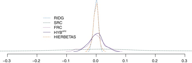
Kernel density estimate of the 91 elements of , , , and , the hybrid estimator without the non-negativity constraint (Remark6.1), from the data analysis. , with the non-negativity constraint, is identically equal to .

Finally, we generated 95% prediction intervals for each observation in the validation sample, using a bootstrap algorithm described in Appendix E of supplementary material available at Biostatistics online. For hierbetas, draws from the posterior distribution of β₀, β, and σ² naturally yield prediction intervals for future observations. Table2 gives the proportion of intervals which included the outcome and the average interval ranges. ridg/hyb have slight under-coverage (0.91), and src and frc have over-coverage (respectively , 1.00 and 0.98). hierbetas is closest to nominal, with 0.94.

Remark 6.1 —

As in the simulation study, we restricted our optimization of ω to the subspace of non-negative elements, which on average improves numerical results. In the data analysis, removing the constraint yields and an MSPE of 0.601. These unconstrained results are also presented in Table2 and Figure3 denoted as hyb^unc.

7. Discussion

Augmenting high-dimensional data with external auxiliary information is useful to boost predictive accuracy. We have described how to quantify this auxiliary information using important ideas from the ME and shrinkage literature. The regression calibration algorithm, src, yields unbiased estimates of future outcomes but with large variance when p is large. A modified algorithm, frc, makes a bias-variance trade-off and can give a smaller MSPE. We have also proposed a hybrid estimator, hyb, which is a linear combination of multiple estimators.

The Bayesian ridge regression, hierbetas, proved to be competitive with hyb and typically had smaller MSPE. Also, prediction intervals using hierbetas are automatic with draws from the posterior distribution. For the TR methods and hyb, a simple bootstrap algorithm yields prediction intervals but requires some modifications to achieve nominal coverage rates.

Despite this, there are reasons to recommend hyb. First, hyb is flexible: it is a linear combination of estimators, each of which can make different modeling assumptions. For example, ridg assumes only the outcome regression model in (1.1), frc additionally assumes the ME model in (1.2), and src assumes these two models plus the marginal model: X∼N_p{μ_X,Σ_X}. Estimators with different modeling assumptions, beyond what we have proposed in this paper, can also be included in hyb, and, from Theorem3.1, it will theoretically do better than the best of any of these. hierbetas does not benefit from this robust model-averaging property. Practically, the average performance of hyb across all design and data configurations is encouraging, and, importantly, its flexibility is most apparent in the large p scenarios. Second, and more significantly, hyb is very fast to compute, whereas hierbetas requires considerably more computational effort. Finally, because hyb combines TR estimators, a GCV criterion provides a simple estimate of P, the prediction error matrix (3.2), which is required to optimize with respect to ω. In our current research, we are exploring an improved GCV criterion which avoids the tendency of GCV to overfit in small-sample scenarios. This has potential to further improve estimates of P and, consequently, prediction for hyb. Alternatively, the “632 estimator” of Efron (1983) is another candidate for estimatingP.

Of potential concern is that we have applied our methods, developed for continuous endpoints, to a dataset with censored survival time as the endpoint. In much the same way as ridge regression has been applied to logistic and Cox models, the TR class may also be adapted to other endpoints. While our theoretical and numerical results have focused only on continuous endpoints, we believe that the ideas and intuition developed will generally transfer to these other endpoints. However, the extension is non-trivial and merits in-depth research, not only for deriving estimators but also in determining the right criterion with which to assess prediction.

Supplementary material

Supplementary material is available at http://biostatistics.oxfordjournals.org.

Funding

This work was supported by the National Science Foundation [DMS1007494] and the National Institutes of Health [CA129102, CA156608, ES020811].

There was an error in the equation in line 3 of the Figure 2 legend. This has now been corrected. The authors apologize for this error.

References

- Breiman L. Stacked regressions. Machine Learning. 1996;24:49–64. [Google Scholar]
- Buzas J., Stefanski L., Tosteson T. Measurement error. In: Ahrens W. and Pigeot I. (editors) Handbook of Epidemiology. 2005:729–765. . Berlin:Springer. [Google Scholar]
- Carroll R. J., Ruppert D., Stefanski L. A., Crainiceanu C. M. Measurement Error in Nonlinear Models. Boca Raton, FL: Chapman & Hall/CRC; 2006. Monographs on Statistics and Applied Probability. [Google Scholar]
- Casella G. Minimax ridge regression estimation. The Annals of Statistics. 1980;8:1036–1056. [Google Scholar]
- Chen Y.-H., Chatterjee N., Carroll R. J. Shrinkage estimators for robust and efficient inference in haplotype-based case-control studies. Journal of the American Statistical Association. 2009;104:220–233. doi: 10.1198/jasa.2009.0104. [DOI] [PMC free article] [PubMed] [Google Scholar]
- Chen M.-H., Ibrahim J. G. Power prior distributions for regression models. Statistical Science. 2000;15:46–60. [Google Scholar]
- Chen G., Kim S., Taylor J. M. G., Wang Z., Lee O., Ramnath N., Reddy R. M., Lin J., Chang A. C., Orringer M. B. Development and validation of a qRT-PCR classifier for lung cancer prognosis. Journal of Thoracic Oncology. 2011;6:1481–1487. doi: 10.1097/JTO.0b013e31822918bd. and others. [DOI] [PMC free article] [PubMed] [Google Scholar]
- Craven P., Wahba G. Smoothing noisy data with spline functions. Numerische Mathematik. 1979;31:377–403. [Google Scholar]
- Dempster A. P., Schatzoff M., Wermuth N. A simulation study of alternatives to ordinary least squares. Journal of the American Statistical Association. 1977;72:77–91. [Google Scholar]
- Draper N. R., van Nostrand R. C. Ridge regression and James–Stein estimation: review and comments. Technometrics. 1979;21:451–466. [Google Scholar]
- Efron B. Estimating the error rate of a prediction rule: improvement on cross-validation. Journal of the American Statistical Association. 1983;78:316–331. [Google Scholar]
- Frank I. E., Friedman J. H. A statistical view of some chemometrics regression tools. Technometrics. 1993;35:109–135. [Google Scholar]
- Fuller W. A. Measurement Error Models. New York: Wiley; 1987. Wiley Series in Probability and Statistics. [Google Scholar]
- Fumera G., Roli F. A theoretical and experimental analysis of linear combiners for multiple classifier systems. IEEE Transactions on Pattern Analysis and Machine Intelligence. 2005;27:942–956. doi: 10.1109/TPAMI.2005.109. [DOI] [PubMed] [Google Scholar]
- Gelfand A. E. On the use of ridge and Stein-type estimators in prediction. Technical Report. 1986 :Stanford University. [Google Scholar]
- George E. I. Minimax multiple shrinkage estimation. The Annals of Statistics. 1986;14:188–205. [Google Scholar]
- Green E. J., Strawderman W. E. A James–Stein type estimator for combining unbiased and possibly biased estimators. Journal of the American Statistical Association. 1991;86:1001–1006. [Google Scholar]
- Gruber M. H. J. Improving Efficiency by Shrinkage: The James–Stein and Ridge Regression Estimators. New York: Marcel Dekker; 1998. [Google Scholar]
- Hoerl A. E., Kennard R. W. Ridge regression: biased estimation for nonorthogonal problems. Technometrics. 1970;12:55–67. [Google Scholar]
- James W., Stein C. Proceedings of the Fourth Berkeley Symposium on Mathematical Statistics and Probability. Volume 1. University of California Press; 1961. Estimation with quadratic loss; pp. 361–379. [Google Scholar]
- LeBlanc M., Tibshirani R. Combining estimates in regression and classification. Journal of the American Statistical Association. 1996;1996:1641–1650. [Google Scholar]
- Li K.-C. Asymptotic optimality of CL and generalized cross-validation in ridge regression with application to spline smoothing. The Annals of Statistics. 1986;14:1101–1112. [Google Scholar]
- Mallows C. L. Some comments on CP. Technometrics. 1973;15:661–675. [Google Scholar]
- Maruyama Y., Strawderman W. E. A new class of generalized Bayes minimax ridge regression estimators. The Annals of Statistics. 2005;33:1753–1770. [Google Scholar]
- Rao C. R. Generalisation of Markoff's theorem and tests of linear hypotheses. Sankhyā. 1945;7:9–16. [Google Scholar]
- Rao C. R. Simultaneous estimation of parameters in different linear models and applications to biometric problems. Biometrics. 1975;31:545–554. [PubMed] [Google Scholar]
- Schäfer J., Strimmer K. A shrinkage approach to large-scale covariance matrix estimation and implications for functional genomics. Statistical Applications in Genetics and Molecular Biology. 2005;4 doi: 10.2202/1544-6115.1175. Article 32. [DOI] [PubMed] [Google Scholar]
- Sclove S. L. Improved estimators for coefficients in linear regression. Journal of the American Statistical Association. 1968;63:596–606. [Google Scholar]
- Swindel B. F. Good ridge estimators based on prior information. Communications in Statistics. 1976;5:1065–1075. [Google Scholar]
Associated Data
This section collects any data citations, data availability statements, or supplementary materials included in this article.