

Abstract
Sample size calculations are an important part of research to balance the use of resources and to avoid undue harm to participants. Effect sizes are an integral part of these calculations and meaningful values are often unknown to the researcher. General recommendations for effect sizes have been proposed for several commonly used statistical procedures. For the analysis of  tables, recommendations have been given for the correlation coefficient
  for binary data; however, it is well known that
  suffers from poor statistical properties. The odds ratio is not problematic, although recommendations based on objective reasoning do not exist. This paper proposes odds ratio recommendations that are anchored to
  for fixed marginal probabilities. It will further be demonstrated that the marginal assumptions can be relaxed resulting in more general results.
Introduction
Sample size calculations are an integral part of scientifically useful and ethical research [1]. A study which is too small may not answer the research question, wasting resources and potentially putting participants at risk for no purpose [2]. Studies which are too large can also waste resources and expose participants to the potential harms of research needlessly, as well as delaying results and their translation into practice. The computation of sample size a priori is usually dependent upon predetermined values for power and level of significance, an estimate of the expected variability in the sample and an effect size of practical or clinical importance. By convention, the choice of power and level of significance is usually at least  and no more than
  respectively. When a practically important effect size is unknown, there are several recommendations in the literature to guide the researcher. In his seminal paper, Cohen [3] gives operationally defined small, medium and large effect sizes for various, common significance tests. The use of effect size recommendations should not replace differences of clinical or practical importance [4] and may not be appropriate for all disciplines. In basic science research, for example, large effect sizes by Cohen's criteria are common and, therefore, require small sample sizes. On the other hand, clinical and epidemiological research often deals with small effect sizes and often requires large, population-based studies. While there are some approaches to estimating a minimum important effect [5], there are instances where this information is simply not known. Thus, effect size recommendations assist with the balance between overly small and overly large sample sizes.
When the researcher is interested in  contingency tables, a common measure of effect size is
  which, in this instance, is equivalent to Pearson's correlation coefficient [6]. Cohen [3] recommends effect sizes of
  and
and  for small, medium and large effect sizes respectively and are identical to his recommendations for the correlation coefficient. Although Cohen [3] denotes this statistic as
  , much of the literature uses
  [6]–[10] and the remainder of this manuscript follows this convention. To support his recommended effect sizes for correlation coefficients, Cohen [11] chose equivalent values for the difference in two means through the connection with point biserial correlation. Additionally,
  is applicable to logistic regression since it can be converted to an odds ratio (
 ) when the row (or column) marginal probabilities of the
  table are fixed. For example, when the marginal probabilities are uniform (i.e.,
  for row and column probabilities), Cohen's recommended effect sizes are equivalent to odds ratios of
  and
and  . It will be demonstrated that the connection between the odds ratio and
  is largely dependent on the marginal probabilities and these
  values should not be used in general.
A problem arises when using the effect size  for
for  tables as the full range of correlation coefficients are only possible under very restrictive circumstances and are not justified in general [12]. On the other hand, odds ratios are valid effect size measures that are not constrained by the marginal probabilities. Ferguson [10] recommends small, medium, and large odds ratio effect sizes of
  and
and  , but urges caution in their use as they are not “anchored” to Pearson's correlation coefficient. Although many have pointed out problems with
  as an association measure and advocate the use of odds ratios as an alternative, effect size recommendations for odds ratios do not exist in general.
It is common in randomised controlled trials and case-control studies to fix one of the marginal probabilities in the  table as it directly relates to the ratio of participant allocation. For instance, a marginal probability of
  corresponds to a 1:1 case-control ratio while a 2:1 ratio is a marginal probability of
  (or equivalently
  for 1:2).
The aims of this paper are to demonstrate: (1) the equivalence of effect size measures for  contingency tables, in particular the relationship between
  and the odds ratio; (2) that recommended odds ratio effect sizes can be derived from Cohen's work using the maximum value of
  as a guideline for fixed marginal probabilities; (3) the shortcomings of
  and the strength of the odds ratio as an effect size measure; and (4) that conservative odds ratio effect size recommendations can be derived without relying on fixed margins. We provide an example that investigates the association between helmet wearing by bicyclists and overtaking distance by automobiles.
Equivalence of Effect Size Measures for 2×2 Contingency Tables
 Contingency tables
The two-way classification or contingency table is a common method for summarising the relationship between two binary variables, say  and
and  . Table 1 gives the joint probability distribution of
  and
and  when their individual outcomes are from the set
  .
.
Table 1. 2×2contingency table of probabilities.
| X = 0 | X = 1 | Total | |
| Y = 0 | π00 | π01 | π0+ |
| Y = 1 | π10 | π11 | π1+ |
| Total | π+0 | π+1 | 1.0 |
In this formulation,  , for
, for  , is the joint probability of
  and
and  ,
,  is the marginal probability of
  , and
, and  is the marginal probability of
  . Under an assumption of independence between
  and
and  , the product of the marginal probabilities equals the cell probabilities, i.e.,
  . Alternatively, the
  table could be represented by the frequency of observations so that
  where
where  . Similarly, the marginal frequencies are
  and
and  . Note that
  is assumed to be the population proportion as the focus of this paper is the use of effect sizes as a planning tool and not statistical inference per se. In a case-control study, for example,
  may indicate the presence or absence of disease while
  is an indication of exposure. Thus,
  would represent the joint probability of being diseased and exposed.
Effect size  and Equivalences for
  Tables
There are many association measures applicable to  tables which, with the exception of the odds ratio and relative risk, are equivalent or similar to
  . The equivalence of some of these association measures is outlined below.
For the random sample  , Pearson's correlation coefficient is
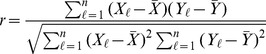 |
where  and
and  are the sample means of the
  and
and  respectively. Although used primarily as a measure of linear association, Pearson's correlation coefficient can be applied to binary variables and is often given the notation
  . For the
  table case, we get
So, Pearson's correlation coefficient for binary random variables  and
and  is
is
Since  under the hypothesis of independence,
  can be interpreted as measuring the departure from independence between
  and
and  . Note that Cramér's
  is equivalent to this equation for the
  table case [11] as well as the square root of Goodman and Kruskal's
  [13].
[13].
For the analysis of contingency tables, in general (not just the  table case) the effect size formula for
  total cells is
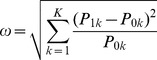 |
where  and
and  are cell probabilities under the null and alternative hypotheses respectively. Note that
  is related to the usual chi-square statistic
  by
by  and is sometimes called the contingency coefficient. Using this formula, Cohen [3] recommends
  and
and  for small, medium and large effect sizes. Making note that
  is the probability of each cell (
 ) and
) and  is the cell probability under an independence assumption (so that
  ), we can then write the effect size formula for the
  table as follows
 |
Simple arithmetic demonstrates the equivalence of  with
with  . The
. The  function is used to give the appropriate sign since the chi-square statistic is inherently non-directional.
The relationship of  to the odds ratio
The odds ratio for the association between  and
and  is
is  . When the marginal probabilities are held constant and the cell probability
  is known, the remaining cell probabilities can be written as
Therefore, when the marginal probabilities are fixed, the odds ratio can be computed directly from  , which can then be expressed as
It is clear from the above formula that the odds ratio will be greater than one (or less than one) precisely when the joint probability  is greater (or less) than expected under an assumption of independence, i.e.,
  . Additionally, the formula for
  can be rearranged to solve for
  , i.e.,
Although mathematically unattractive, it is clear the odds ratio can then be computed from  ,
,  , and
, and  . Note that when
  (i.e., no correlation), we get
  (i.e.,
  and
and  are independent) and the odds ratio is
  . When
  , the term
  is then a measure of the departure from independence.
Maximum  and Modified Effect Sizes
When the marginal probabilities are fixed constants,  is an increasing linear function of
  . Further,
  is bounded by
These bounds are due to all cell probabilities being non-negative and the relationship of  with the other cell probabilities given above. As a result,
  is bounded as well and attains its maximum when
  . Using the upper bound of the above inequality, it can be shown that
 |
where  to ensure
  . It is clear from the formula for
  that the full range of correlation coefficients, i.e.,
  , is attainable only when the marginal probabilities are equal, i.e.,
  or
or 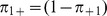 . This has an intuitive appeal as perfect correlation for two binary variables is only possible when two cell probabilities are zero. For example, when all observations are in either the
  or
or  cells,
  . However, it would appear highly unlikely both marginal probabilities will be equal in practice. For example, in a 1:1 case-control study with mortality as the primary outcome, half of all patients would need to die for perfect correlation to be possible. On the other hand, if
  of all patients die, the maximum correlation possible is
  which is near a medium recommended effect size. So, in this situation, all estimates of
  , computed from observed proportions, are bounded by
Importantly, odds ratios are not bounded with possible values of  as
as  varies on the interval
  . In fact, as
  approaches
  , the
, the  increases without bound. Figure 1 demonstrates this relationship. Importantly, this indicates
  has serious limitations as a measure of association and that these limitations are not applicable to the odds ratio.
Figure 1. Relationship between the odds ratio and  for unequal marginal probabilities.

Effect Sizes Relative to 
In many practical instances, the marginal probabilities are not equal, making the full range of values for  impossible with the potential of making Cohen's recommended effect sizes unusable for
  tables. Although not equivalent to perfect correlation,
  can be interpreted as the maximum possible correlation given the marginal probabilities. In fact,
  /
/ has been proposed as an association measure with the interpretation as the proportion of observed correlation relative to the maximum attainable with fixed marginal probabilities [7], although the researcher is cautioned when the marginal probabilities diverge [6]. Note that
  is not equivalent to Cohen's similarity/agreement measure
  . However,
  suffers from the same boundary problems as
  and the two are equivalent when scaled to their maximum values, i.e.,
  /
/ /
/ , making the two measures similar [6].
Recommended effect sizes in terms of the odds ratio
As an alternative to Cohen's recommendations, increments of  can be related to the odds ratio, say
  , where
  . Note that values of
  or
or  coincide with Cohen's usual recommendations when
  . The relationship between
  and the odds ratio can be simplified by choosing marginal probabilities for commonly used participant allocations. As an example, Figures 2 and 3 demonstrate the relationship between
  and odds ratios for
  ,
,  and
and  for 1:1 and 1:2 allocations respectively. Note that the minimal odds ratios, and therefore most conservative when used to compute sample size, occur when
  tends to
  . Although the odds ratio does not exist when
  , the limit exists and is
Figure 2. Odds ratios and marginal probability by small, medium and large effect sizes for 1:1 allocation.

Figure 3. Odds ratios and marginal probability by small, medium and large effect sizes for 1:2 allocation.

Additionally, the maximal odds ratio, and therefore most anti-conservative, occurs when the marginal probabilities are equal, as expected. Below is the maximum attainable odds ratio for equal margins  for increments
  of
of  ,
,
It is important to note that when  , as is often true for case-control studies where cases are harder to identify or enrol than controls, the minimal odds ratio will be smallest for evenly allocated studies, i.e.,
  . Further, it is generally recommended to use 1:1 allocation as it is the most statistically efficient ratio, i.e., maximum power for a fixed overall sample size. So, odds ratios of
  and
and  can be used as small, medium and large effect sizes without assumptions regarding marginal probabilities. Sample sizes computed using these odds ratios for 1:1 allocation are given in Table 2 for
  power and
  level of significance. A SAS macro that will compute sample sizes from given marginal probabilities for small, medium and large odds ratios has been provided as a supplementary file.
Table 2. Sample sizes calculated for small, medium and large effect sizes for 1:1 allocation, 80 power and
  .
.
| π1+ | |||||||||
| Odds Ratio | 0.1 | 0.2 | 0.3 | 0.4 | 0.5 | 0.6 | 0.7 | 0.8 | 0.9 |
| 1.22 | 8168 | 4688 | 3646 | 3254 | 3188 | 3386 | 3948 | 5282 | 9576 |
| 1.86 | 724 | 436 | 354 | 330 | 338 | 374 | 454 | 632 | 1188 |
| 3.00 | 200 | 128 | 110 | 108 | 116 | 134 | 170 | 246 | 480 |
Interestingly, Haddock et al. [12] as a rule of thumb consider odds ratios greater than  large effect sizes, although there is no clear justification given. In a situation where an allocation ratio other than 1:1 is used, recommended odds ratios can be computed directly using the above formula. These results are also applicable for other values of
  through its complement
  . This is equivalent to swapping the columns (or rows) and the researcher should be aware the recommended odds ratio effect sizes are now the reciprocals of those above, i.e.,
  and
and  for small, medium and large respectively.
This approach can also be applied to the relative risk and risk difference. If  is taken as the grouping variable and
  as the outcome, the relative risk is
 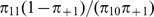 . Simple substitution of
  and the marginal probabilities
  and
and  results in a relative risk identical to
  for
for  , i.e.,
Therefore, recommendations can also be derived for relative risk and are identical to those given for the odds ratio above. This result is expected as the odds ratio converges to the relative risk as the incidence rate approaches  .
.
Instead of comparing the risk between two groups as a ratio, it is sometimes useful to compare their differences [14]. Again taking  as the grouping variable and
  as the outcome, the risk difference can be written as
where  to ensure
  as above. It is clear from the numerator in this representation that
  is a measure of the departure from independence, i.e.,
  . Simple substitution of
  into
into  yields
where the subscript  is used to distinguish between risk difference formulae. This formula can be simplified somewhat for 1:1 allocations, i.e.,
  ; however, a general result independent of the marginal probabilities is clearly not possible in this instance as
  and therefore
 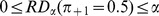 .
.
Alternatively, the  formula can be solved for
  and compared to previously given odds ratio recommendations. In terms of
  and
and  , we get
When the allocation ratio is 1:1, this formula simplifies to  which has a form identical to Yule's
  [15]. So, Ferguson's [10] odds ratio recommendations of
  and
and  therefore correspond to proportions of maximum correlation of
  and
and  . This suggests Ferguson's recommendations have the potential to be anti-conservative from a sample size viewpoint.
Example
This paper was motivated by a reanalysis of passing distances for motor vehicles overtaking a bicyclist [16]. One of the primary results of this study was a significant association between helmet wearing and less overtaking distance, supporting a theory of risk perception for motor vehicle drivers directed towards bicyclists. Prior to collecting data, Walker [16] reported computing a sample size of  overtaking manoeuvres based on a
  fixed effects factorial ANOVA for a small effect size
  ,
,  level of significance and
  power. The factors for this study were helmet wearing (2 levels) and bicycle position relative to the kerb (5 levels). It has been noted, however, that passing distances are often recommended and sometimes legislated to one metre or more [17]. So, passing manoeuvres of at least a metre are considered safe and less than a metre unsafe, with the implication that large differences in passing distance are unimportant beyond one metre in terms of bicycle safety. When compared with helmet wearing, safe/unsafe passing distances can be analysed using a
  table. Since Walker's study was powered at an unusually high level with subsequent increased probability of a type I error, bootstrap standard errors were estimated for more reasonable values for power of
  ,
,  and
and  . Operationally defined small, medium and large effect sizes were also used since a meaningful difference in overtaking distance is unknown.
The relevant observed data from Walker [16] is given in Table 3. The observed marginal proportions here are  for helmet wearing and
  for unsafe passing manoeuvres. Using the marginal probabilities, the maximum attainable effect size is
  and the estimated correlation is
  . A consequence is the effect size for the association between helmet wearing and safe passing distance is, at best, much less than a small effect size by Cohen's index. The corresponding small, medium and large odds ratio effect sizes using increments of
  are
are  and
and  for
for  and
and  . Note that these values are not much greater than the minimal recommended odds ratios mentioned in the previous section, further suggesting the association between safe/unsafe passing distance and helmet wearing is, at best, a small effect size. In fact, the unadjusted odds ratio is
  and non-significant by the chi-square test (
 ). Conversely, sample sizes for a future study can be computed from the observed probabilities using G*Power for logistic regression with a single binomially distributed predictor for
  and
and  power [18] resulting in
  and
and  observations for small, medium and large odds ratios. To put these sample size computations into perspective, a future study would need to extend the sampling period by a factor greater than seven to detect a significant association between helmet wearing and safe/unsafe overtaking distance given a small effect size and identical marginal probabilities.
Table 3. Observed proportion of helmet use and safe passing manoeuvres from Walker (2007).
| No Helmet | Helmet | Total | |
| Safe | 0.491 | 0.462 | 0.953 |
| Unsafe | 0.021 | 0.026 | 0.047 |
| Total | 0.512 | 0.488 |
Discussion
We present a demonstration that many contingency table correlation measures are equivalent for the  case and their use is limited due to constraints created by fixed marginal probabilities. The odds ratio, which is a function of these measures for fixed marginal probabilities, is not problematic, is regularly used in statistical analyses and has a direct application to logistic regression. Recommended odds ratios have been proposed from Cohen's small, medium and large effect sizes for
  relative to the maximum attainable correlation
  . Further, minimal odds ratios can be computed with only knowledge of participant allocation.
The use of effect size recommendations should be avoided in situations in which clinical or practical differences are known. However, they can help the researcher balance between overly large or overly small sample size calculations when such information is unknown. In these situations, conservative estimates for odds ratio effect sizes can be derived from only the allocation ratio leading to a general result and, when a 1:1 allocation is chosen for optimal power, odds ratios of  and
and  correspond to small, medium and large effect sizes.
Supporting Information
SAS Macro to compute sample sizes from marginal probabilities for small, medium and large odds ratios.
(SAS)
Acknowledgments
The authors would like to thank Warren May, David Warton and Jakub Stoklosa for their help in the preparation of this manuscript.
Funding Statement
The authors have no support or funding to report.
References
- 1. Lewis J (1999) Statistical principles for clinical trials (ICH E9): an introductory note on an inter-national guideline. Statistics in Medicine 18: 1903–1942. [DOI] [PubMed] [Google Scholar]
- 2. Halpern S, Karlawish J, Berlin J (2002) The continuing unethical conduct of underpowered clinical trials. JAMA: The Journal of the American Medical Association 288: 358–362. [DOI] [PubMed] [Google Scholar]
- 3. Cohen J (1992) A power primer. Psychological Bulletin 112: 155–159. [DOI] [PubMed] [Google Scholar]
- 4. Lenth R (2001) Some practical guidelines for effective sample size determination. The American Statistician 55: 187–193. [Google Scholar]
- 5. King M (2011) A point of minimal important difference (MID): a critique of terminology and methods. Expert Review of Pharmacoeconomics & Outcomes Research 11: 171–184. [DOI] [PubMed] [Google Scholar]
- 6. Davenport Jr E, El-Sanhurry N (1991) Phi/phimax: review and synthesis. Educational and Psy-chological Measurement 51: 821–828. [Google Scholar]
- 7. Ferguson G (1941) The factorial interpretation of test difficulty. Psychometrika 6: 323–329. [Google Scholar]
- 8. Guilford J (1965) The minimal phi coefficient and the maximal phi. Educational and Psychological Measurement 25: 3–8. [Google Scholar]
- 9. Breaugh J (2003) Effect size estimation: Factors to consider and mistakes to avoid. Journal of Management 29: 79–97. [Google Scholar]
- 10. Ferguson C (2009) An effect size primer: A guide for clinicians and researchers. Professional Psychology: Research and Practice 40: 532–538. [Google Scholar]
- 11.Cohen J (1988) Statistical Power Analysis for the Behavioral Sciences. Hillsdale, New Jersey: Lawrence Erlbaum Associates.
- 12. Haddock C, Rindskopf D, Shadish W (1998) Using odds ratios as effect sizes for meta-analysis of dichotomous data: A primer on methods and issues. Psychological Methods 3: 339–353. [Google Scholar]
- 13.Agresti A (2002) Categorical Data Analysis. New York: Wiley-interscience.
- 14.Greenberg R, Daniels S, Flanders W, Eley J, Boring J (1996) Medical Epidemiology. Appleton & Lange.
- 15.Liebetrau A (1983) Measures of Association, volume 32. Sage Publications, Incorporated.
- 16. Walker I (2007) Drivers overtaking bicyclists: Objective data on the effects of riding position, helmet use, vehicle type and apparent gender. Accident Analysis & Prevention 39: 417–425. [DOI] [PubMed] [Google Scholar]
- 17.Olivier J (2013) Bicycle helmet wearing is not associated with close overtaking: A re-analysis of Walker 2007. Submitted. [DOI] [PMC free article] [PubMed]
- 18. Faul F, Erdfelder E, Buchner A, Lang A (2009) Statistical power analyses using G*Power 3.1: Tests for correlation and regression analyses. Behavior research methods 41: 1149–1160. [DOI] [PubMed] [Google Scholar]
Associated Data
This section collects any data citations, data availability statements, or supplementary materials included in this article.
Supplementary Materials
SAS Macro to compute sample sizes from marginal probabilities for small, medium and large odds ratios.
(SAS)