From next-generation sequencing alignments to accurate comparison and validation of single-nucleotide variants: the pibase software

Abstract

Scientists working with single-nucleotide variants (SNVs), inferred by next-generation sequencing software, often need further information regarding true variants, artifacts and sequence coverage gaps. In clinical diagnostics, e.g. SNVs must usually be validated by visual inspection or several independent SNV-callers. We here demonstrate that 0.5–60% of relevant SNVs might not be detected due to coverage gaps, or might be misidentified. Even low error rates can overwhelm the true biological signal, especially in clinical diagnostics, in research comparing healthy with affected cells, in archaeogenetic dating or in forensics. For these reasons, we have developed a package called pibase, which is applicable to diploid and haploid genome, exome or targeted enrichment data. pibase extracts details on nucleotides from alignment files at user-specified coordinates and identifies reproducible genotypes, if present. In test cases pibase identifies genotypes at 99.98% specificity, 10-fold better than other tools. pibase also provides pair-wise comparisons between healthy and affected cells using nucleotide signals (10-fold more accurately than a genotype-based approach, as we show in our case study of monozygotic twins). This comparison tool also solves the problem of detecting allelic imbalance within heterozygous SNVs in copy number variation loci, or in heterogeneous tumor sequences.

INTRODUCTION

The first step in next-generation sequencing (NGS) of genomic DNA is the massively parallel sequencing of millions to billions of short DNA fragments on a single platform, typically generating short sequences (termed ‘reads’) from each end of the DNA fragment. For quality control purposes, the NGS platforms also generate quality values for every sequenced base, in analogy to the capillary sequencing quality values that are named after the phred software (1). The second step, which involves a high-performance workstation or a compute cluster, is to determine the most probable genomic origin of each fragment by aligning the reads to a reference, typically to the sequences of a whole genome. Automatic, fast and error-tolerant alignment methods such as the Burrows-Wheeler Aligner (BWA) exist (2), enabling the huge numbers of reads to be aligned within a reasonable time span. The third step, also carried out on a workstation or a compute cluster, is the identification (‘calling’) of variants from the resulting alignments. This variant-calling is not straightforward, because of existing experimental and platform differences, alignment ambiguities and biological particulars such as ploidy changes in tumors and in double minutes [tiny ‘extra’ chromosomes that may contain segmental copies of chromosomes and are replicated during cell division, see (3–5)]. Typically, single-nucleotide variant (SNV)-calling algorithms, such as in SOLiD Bioscope, the SAMtools software (6), the Genome Analysis Toolkit (GATK) (7) and VarScan (8), generate SNV-lists using filtering or probabilistic methods to exclude artifacts. These software tools generally contain pre-set filters to detect variations.

Quality control (QC) of NGS SNV data is vital and by definition, needs to be performed independently of the data production. For example, in clinical diagnostics, SNVs must usually be validated by visual inspection or several independent SNV-callers. Human geneticists are normally forced to store and present the raw sequence data for the mutation of interest. To this end, chromatograms are attached to clinical reports for Sanger-based tests. For NGS, pibase yields accurate read statistics for a genomic SNV of interest. As a matter of note, the SNVs released by the 1000 Genomes Project (9) were a consensus from at least two different groups, two different NGS platforms and two different bioinformatic pipelines, significantly reducing the risk of human errors, platform errors and software errors, respectively. Data exchange errors within the 1000 Genomes Project were mitigated by developing shared conventions, including the current standard alignment file format, Binary Sequence Alignment/Map (BAM) (6) and the Variant Call Format (VCF) (10). Further strategies and tools for QC, including contamination detection using the pibase tools, are discussed in the Supplementary Methods. Currently, ‘one of the main uses of next-generation sequencing is to discover variation among large populations of related samples’ (10) and for this purpose, probabilistic frameworks exist (7,11,12) that help to separate good novel SNV candidates from likely false positives (artifacts) and to determine allele frequencies in populations.

Unfortunately, there are several challenges when faithfully applying the variation–discovery approaches to other uses, such as clinical diagnostics, forensics and targeted-sequencing-based phylogenetic analyses. To begin with, the filtered SNV-lists generated by these approaches do not include low-confidence genotypes, e.g. where both-stranded validation is missing, and the unwary data recipient may interpret missing information as a reference sequence genotype. Also, the default filters sometimes eliminate obvious genotypes (Supplementary Tables S1 and S2; Supplementary Figures S1 and S2). The second problem is that available variant-calling tools usually do not list sequencing failures, where there is low coverage or no coverage at all, and the unwary data recipient may again interpret this omission as a reference sequence genotype. These two errors alone can amount to high error rates, e.g. 59.3% (Supplementary Table S3d) in an older whole genome sequencing run, or 9.5% (Supplementary Table S4) in a recent Illumina HiSeq 2000 exome sequencing run. We have noticed that targeted sequencing data are much more prone to these errors than recent whole genome sequencing data at only 0.5% error (Supplementary Table S3a–c). A third problem is that SNV-lists usually include incorrectly identified heterozygotes (prompted by an occasional sequencing error, misalignment or contaminant sequence) where the pre-set quality filter for machine output or read-alignment is inappropriate. The fourth problem occurs when the user employs several different SNV-callers to perform a basic validation of the SNV-lists by intersecting the individual SNV-lists to separate cross-validated SNVs from less validated ones. Because each of these individual tools is, as explained above, prone to filtering away valid SNVs, the intersected consensus genotypes will exclude even more valid SNVs.

When performing comparisons between healthy and affected cells/individuals, a fifth problem surfaces, as each of the first four problems will lead to false differences in the comparative analyses. In other words, for such comparisons, it may not be advisable to rely on derived SNV-lists. Instead, the underlying BAM files are needed. Going back to the BAM files also resolves the sixth and most important problem: a specific challenge in cell or proband comparisons is to detect significant changes of allelic balance in heterozygous SNVs, e.g. in heterogeneous tumor samples or in the case of copy number variation loci. Only the primary BAM file but not the derived SNV-lists can re-create this proportion of alleles.

Finally, if there is a communication bottleneck between NGS bioinformaticians (data producers) and other scientists/clinicians (data users), this may result in unnecessary analysis reruns with new work flows or filtering parameters, specifically when new people or new NGS experiments are involved.

We have therefore, developed the pibase package (http://www.ikmb.uni-kiel.de/pibase, 23 August 2012, date last accessed), which, instead of relying on a single set of filtering parameters, applies 10 sets of filtering parameters and then infers the best genotype or the best comparison; complements the available general data analysis tools; saves considerable manual validation work and, unlike the manual approach, can be integrated into a bioinformatic pipeline. pibase was developed as a consequence of our previous study (13): there, we systematically evaluated the stability of SNV-calls by observing all reads and all unique start points, as well as seven randomly sampled subsets of reads and unique start points yielding average coverages of 100×, 80×, 60×, 40×, 20×, 10× and 5×, respectively. Independently of the sequencing platform, genotype changes suddenly began to occur when coverages were reduced to 20× or lower (13). This coverage-related genotype instability ultimately affected ∼10% of the SNVs when the coverage was lowered to 5× (13).

In Figure 1, we present pibase’s ‘essential’ workflow (the prerequisite for all other workflows), in which pibase accepts BAM files and then extracts and tabulates nucleotide signals at genomic coordinates of interest using 10 different observation methods or ‘filters’ (from which pibase infers its ‘best genotype’): pibase observes reads and unique start points using five distinct and increasingly stringent quality filters (Table 1). The resulting information is not restricted to a single stringency or a single filter setting, and is therefore, more complete and less biased than information from single-source SNV-lists or manual inspections. Additionally, reference sequence information is included in this table, which pibase requires and which, as a bonus, also reduces the need for manual inspections in a viewer. Table 1 demonstrates pibase filtering and the resulting coverage at four positions, representing the bandwidth from acceptable coverage to unacceptably low coverage. Filtering improves genotyping accuracy by eliminating potential errors in the raw reads and the alignments, but at the cost of reducing the number of remaining reads. In Table 1, filtering stringency increases from left to right, as explained in the ‘Materials and Methods’ section (pibase_bamref). Coverage is not uniform over the genome, making the identification of some genotypes less confident than others (Table 2). A genotype is inferred for each of the 10 filter methods, which ideally all should result in identical genotypes. A summary ‘best genotype’ and its quality are computed from these 10 observations. Table 2 shows the per-filter genotype evaluated from the read counts in Table 1, and the resulting pibase consensus genotype and quality grade. The columns with Filters 1 and 3 are not shown in this example. For directly comparing two data sets, e.g. patients versus healthy controls in disease association studies, pibase uses a statistical approach on filtered read counts (original data) with associated quality control criteria, rather than a simple comparison of SNV-lists (processed data). We implemented this comparison method because, we observed that SNV-calls or allele-calls may be suppressed in one of the samples being compared, merely because of stringency filters and coverage differences. Our approach should not be confused with the one implemented in CRISP (14), which dramatically improves the accuracy of rare variant-calling in pools using Fisher’s exact test on A- and B-allele counts and multiple pools of samples. It is also not the same as the genotype-free likelihood-based approaches for pairwise comparisons and family trio comparisons that have been recently implemented by Li (11). In summary, pibase addresses major problems pertaining to the quality control, validation and accurate comparison of NGS variant data, which are a bottleneck in currently emerging translational uses of NGS. Furthermore, the pibase data tables facilitate the practical use of NGS data by non-bioinformaticians such as archaeogeneticists, biologists, clinicians and forensic scientists.

Figure 1.

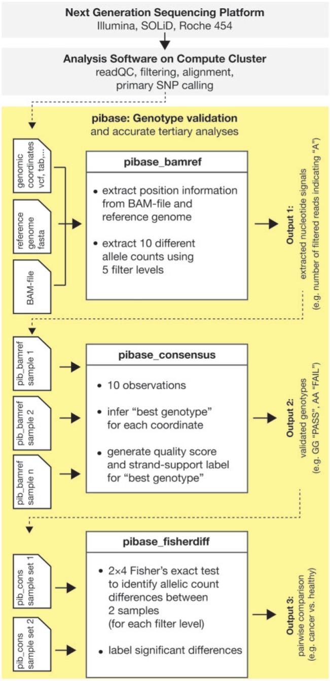
Flow chart showing the standard NGS sequencing and bioinformatic analysis (gray). The ‘essential workflow’ of pibase (yellow): pibase_bamref reads a list of genomic coordinates from a tab-separated text file, a VCF file, a SAMtools pileup SNV file or a Bioscope gff3 SNV file. It then extracts data from a reference sequence file and a sequence alignment (BAM) file and outputs extracted, computed and filtered information as a tab-separated text file (output 1). pibase_consensus reads one single or several pibase_bamref files. For each coordinate, a ‘best genotype’ with quality and strand support, as well as two genotypes for each filter level are inferred, and these data are appended to the pibase_bamref data (output 2). pibase_fisherdiff is a tool for association testing or sample comparison, requiring a pair of pibase_consensus files as input data (e.g. case/control, germline/tumor or affected/unaffected twin). The tool appends P-values and a filter label to the pibase_consensus data (output 3). Further workflows address annotation and phylogenetic analysis.

Table 1.

Remaining reads after successive filtering at four positions in a public BAM file

Genomic coordinate	Raw	Filter 0a		Filter 1b		Filter 2c		Filter 3d		Filter 4e
	CV	CV	SP	CV	SP	CV	SP	CV	SP	CV	SP
chr22:19969075	6	3	3	0	0	0	0	0	0	0	0
chr22:19969495	14	11	8	8	6	3	2	3	2	3	2
chr22:30857373	8	5	5	2	2	1	1	1	1	1	1
chr22:31491295	17	7	7	4	4	3	3	2	2	2	2

^aReads without indels; ^bFilter 0 and base quality ≥ 20; ^cFilter 1 and read length ≥ 34; ^dFilter 2 and mismatches ≤ 1; ^eFilter 3 and uniquely mappable reads. CV: number of (all) reads covering this genomic coordinate; SP: remaining reads after filtering away reads with the same start points.

Table 2.

Stable and instable genotypes resulting from the filtering in Table 1

Genomic coordinate	Filter 0		Filter 2		Filter 4		End resultb		Three platformse
	CV	SP	CV	SP	CV	SP	BGc	Qualityd
chr22:19969075	aaa	aaa					AA	FAIL	AG
chr22:19969495	GG	GG	gga	gga	gga	gga	GG	PASS	GG
chr22:30857373	aca	aca	cca	cca	cca	cca	AC	FAIL	AC
chr22:31491295	cga	cga	cca	cca			CG	FAIL	CG

^aLow coverage; ^brule-based consensus over all filter levels; ^cpibase consensus genotype; ^dpibase PASS/FAIL tag; ^ethe 1000 Genomes Project’s consensus of three sequencing platforms (Illumina, SOLiD, FLX/454) is shown for comparison.

MATERIALS AND METHODS

Overview

The pibase package is structured into workflows and consists of linux command line tools that can be incorporated into sequential pipelines and into linux cluster pipelines. When developing pibase, it was important to have simple commands and meaningful help texts at the command line. Equally important was exception trapping with meaningful error messages.

The ‘essential workflow’ (Figure 1) is complemented by optional workflows and some utilities. The ‘annotate workflow’ adds annotations to outputs 2 or 3 (Figure 1), using the command line version of our internal SNV categorization package snpActs (http://snpacts.ikmb.uni-kiel.de, 23 August 2012, date last accessed). The ‘phylogenetics workflow’ provides a link from NGS data to median joining network analysis (15). This network method is widely used in the field of biology to generate evolutionary tree-like graphics for a population of individuals, in order to stratify the population and uncover evolutionary structures (‘family trees’), ancestral sequences and mutation events of significance. Traditionally, median-joining networks are computed on the basis of mitochondrial markers or short tandem repeats (STR) on the Y-chromosome. These loci are usually sufficiently hyper-variable to discriminate between individuals of the same species. The mitochondrial and Y-chromosomal loci are normally recombination-free, which is the prerequisite for computing the maternal lineage and the paternal lineage, respectively. If an evolutionary network is to be constructed from a single individual’s germ-line and somatic cells, any genomic marker is normally recombination-free within this cell population. Therefore, pibase was designed to translate mitochondrial, Y-chromosomal and diploid SNVs into a generic format for the network analysis software. This network method can be used to compute the evolutionary network of heterogeneous tumor cells within a single patient and identify the ancestral tumor cells, i.e. the link between the healthy germ-line cell and the tumor cell population. More importantly, networks can be used to confirm that different samples from one individual were not confused with samples from other individuals.

Algorithms

We have described the algorithms for each pibase tool in the Supplementary Data, including instructions for using pibase for contamination detection. Details on the pibase data preparation for the Network software can also be found in the Supplementary Data.

Implementation

System requirements and installation instructions are listed under (http://www.ikmb.uni–kiel.de/pibase/index.html#tutorial, 23 August 2012, date last accessed). All tools were written in Python (http://www.python.org/, 23 August 2012, date last accessed). The pibase_bamref tool requires the Python module pysam (http://code.google.com/p/pysam/downloads/list, 23 August 2012, date last accessed). The pibase_fisherdiff tool calls a FORTRAN77 program which uses ‘algorithm 643’ (16) (http://portal.acm.org/citation.cfm?id=214326, 23 August 2012, date last accessed) (with the original workspace increased 1000× to 800 MB) and the DATAPAC library (http://www.itl.nist.gov/div898/software/datapac/homepage.htm, 23 August 2012, date last accessed) and was compiled with the free GNU Fortran compiler (http://gcc.gnu.org/fortran/, 23 August 2012, date last accessed). The RAM memory footprint of the Python tools was explicitly limited to 1 GB, and the FORTRAN77 program is limited to <1 GB.

We have tested the tools on BAM files from the following pipelines and sequencing platforms: ABI SOLiD reads mapped with SOLiD Bioscope (v1.0.1 and v1.2.1) and BFAST (17), Illumina GA II and HiSeq 2000 reads mapped with BWA and SOAP (18) (after conversion using soap2sam.pl and SAMtools) and Roche 454/FLX reads mapped with BWA and SSAHA (19). The pibase tools have been tested within locally ongoing scientific research projects and further tools are being added to the pibase package as needed. Users with questions or suggestions are welcome to contact the authors.

Example data

For our example data download on the project homepage (http://www.ikmb.uni-kiel.de/pibase, 23 August 2012, date last accessed), we used the publicly available BAM files for chromosome 22, (ftp://ftp.1000genomes.ebi.ac.uk/vol1/ftp/technical/pilot2_high_cov_GRCh37_bams/, 23 August 2012, date last accessed), for the high-coverage trio samples from Utah residents with Northern and Western European ancestry (CEU): NA12878 (daughter), NA12891 (father) and NA12892 (mother). The daughter’s whole genome BAM files were available as Illumina, SOLiD and 454/FLX reads, and the father’s and mother’s files were only available as Illumina reads. In the 1000 Genomes Project, the Illumina reads were mapped using BWA, the SOLiD reads using BFAST, and the 454/FLX reads using SSAHA.

The reference sequence used for mapping by the 1000 Genomes Project is available at (ftp://ftp.sanger.ac.uk/pub/1000genomes/tk2/main_project_reference/human_g1k_v37.fasta.gz, 23 August 2012, date last accessed). This genome is largely the same as hg19, except that, e.g. the chromosome names are changed to 1, 2, 3, etc., and the mitochondrial reference sequence is rCRS not chrM. We supply the file hg19.1000 G.quick.fasta in our example data download for use with chromosomes 1–22, X and Y.

We also downloaded the file of exonic variant-calls (CEU.exon.2010_03.genotypes.vcf.gz) from (ftp://ftp.1000genomes.ebi.ac.uk/vol1/ftp/pilot_data/release/2010_07/exon/snps/, 23 August 2012, date last accessed). The VCF file lists only 55 SNVs for chromosome 22, and their genomic coordinates are counted with respect to hg18. We transformed these SNV coordinates to hg19 coordinates using the online tool at (http://genome.ucsc.edu/cgi-bin/hgLiftOver, 23 August 2012, date last accessed) (20) and used them for the pibase analysis examples.

For further comparisons with established results and established tools, we used pibase to recall the HapMap single nucleotide polymorphisms (SNPs, a class of SNVs that occur in at least 1% of individuals in a specific population) defined in hapmap3_r1_b36_fwd.CEU.qc.poly.recode.map (ftp://ftp.ncbi.nlm.nih.gov/hapmap/phase_3, 23 August 2012, date last accessed) after coordinate transformation from hg18/b36 to hg19. For the above whole genome sequencing files, we recalled SNVs in chromosome 22 using both GATK and SAMtools (mpileup, bcftools, vcfutils), merged the GATK and SAMtools SNV-lists (i.e. the union of both SNV-lists, not the overlap) and recalled these SNVs using pibase. As a targeted sequencing example, we used the fastq files available from the EBI/NCBI SRA with the SRA run ID SRR098401 (the high-coverage HapMap CEU trio daughter NA12878, http://www.ebi.ac.uk/ena/data/view/SRR098401, 23 August 2012, date last accessed). These whole exome reads were generated with an Illumina HiSeq 2000 at the Broad Institute, Cambridge, MA, USA. We mapped the reads using BWA (BAM file version 1). We removed duplicates using Picard (BAM file version 2). We removed non-uniquely aligned reads (BAM file version 3). We called SNVs for each BAM file version using SAMtools and GATK with the Variant Quality Score Recalibrator software (VQSR) (12). We used pibase to genotype exonic HapMap SNPs (the genomic HapMap SNPs were filtered to lie within the regions defined by CCDS.20110907.txt, which we downloaded from (ftp://ftp.ncbi.nlm.nih.gov/pub/CCDS/current_human/, 23 August 2012, date last accessed), and then filtered to exclude reference sequence genotypes). We compared all recalled SNVs with the HapMap SNPs in hapmap3_r1_b36_fwd.CEU.qc.poly.recode.ped to assess the levels of specificity. Finally, using PLINK (21), we performed Mendelian error checks for the SNV-lists from the Illumina trio data, to further compare the levels of specificity. We documented the settings for each tool in the shell scripts that are included in our example data download (subfolders chr22_snpcalling, chr22_scripts, and exome).

SNV differences in identical twins

As part of an ongoing research project, the exomes of two German twin pairs were analyzed. The Agilent SureSelect Human All Exon v2 Kit was used for capturing 48 Mb of target regions. The four exome samples were each sequenced on a quadrant of a quartet slide on the SOLiD v4 platform using paired-end reads (50 bp forward, 35 bp reverse). The reads were mapped using Bioscope 1.2.1. Duplicate reads were removed from the BAM files using Picard. SNVs were called using Bioscope 1.2.1 and also SAMtools (pileup), resulting in four SNV-lists per twin pair. These four SNV-lists per twin pair were merged, and pibase was used to interrogate each of these genomic coordinates in each twin of that pair. Finally, pibase was used for two different methods of comparison: the first method using conventional genotype comparison after interrogating the BAM files (pibase_diff) and the second method using Fisher’s exact test of nucleotide signals at five different filter levels in the BAM files (pibase_fisherdiff).

Median joining network analysis

To demonstrate how to check for potential sample confusion if just a small number of discriminating SNVs is available, we employed median joining network analysis (15) to compare the five example 1000 Genomes BAM files, comprising two parents sequenced on Illumina and their daughter sequenced on Illumina, SOLiD and FLX/454. We used the daughter’s Illumina BAM file as the control or reference sample. We used pibase_bamref followed by pibase_consensus for each sample. We then performed pibase_fisherdiff comparisons between the control sample and each of the remaining samples at the 55 genomic coordinates of exonic SNPs reported by the 1000 Genomes Project. We used pibase_to_rdf to generate the rdf files setting p.med ≤0.2 without requesting both-stranded confirmation. We used Network 4.6.0.0 to compute the median joining networks using default settings. Network accepts five main input data formats: ‘binary’ format (1/0 or difference/no difference), ‘multistate’ DNA format (A, C, G, T, N, -), ‘multistate’ amino acid format (A, B, C, D, etc.), restriction fragment length polymorphism (RFLP) format and ‘Y-STR’ format (counts of a repetitive marker motif at a site). pibase_to_rdf can generate the binary format (which is the most efficient format for handling large data sets) and resolves the challenge of defining a difference/no difference criterion for diploid genomic genotype data.

RESULTS

Using pibase, we obtained highly specific (99.97–100.00%) genotype calls from publicly available Illumina GAII BAM files as detailed below in the 1000 Genomes Project example section. We also demonstrate significantly shorter run times to validate genotypes at the specified list of known HapMap SNP coordinates than is required by samtools or GATK for a complete SNP-calling run on chromosome 22. Furthermore, we report that the false discovery rate of SNV differences in pairs of monozygotic twins is 10-fold lower using pibase’s Fisher’s exact test, than using a genotype-based comparison method. Finally, we show that pibase can be used in combination with a phylogenetic network method to sort out potential sample confusions using a set of only 55 SNVs.

Example data from the 1000 Genomes Project

Tables 1–3 show the principles using selected (and simplified) results from pibase_bamref, pibase_consensus and pibase_fisherdiff. Within a single run, pibase_bamref applied multiple filters with increasing stringency and computed the resulting allele counts for each filter stage, shown simplified as coverages in Table 1. The data in Table 1 refer to the NA12878 SOLiD BAM file in our example data download. The genomic coordinates are based on hg19, and the starting coordinate is counted from one. Then, pibase_consensus called a genotype for each filter stage and inferred a consensus genotype (Table 2). pibase inferred the single-platform consensus genotypes in lines one, three and four from low coverage or filtering ambiguities, and marked them as a failure (‘low coverage guess’) because this quality is not acceptable in our opinion. Regarding the genotype in line one, not a single SOLiD read contains the G-allele that was detected on the FLX/454 and the Illumina. The genotype in the second line is unambiguous (stable) over all filters, and is confirmed by sufficient reads. The ambiguous (instable) consensus genotypes in lines three and four were inferred from read-counts at various filter levels and other information.

Table 3.

Discrimination of non-identical SNVs in BAM file pairs using Fisher’s exact test

Genomic coordinate	P-valuea (from read-counts)	Best genotype
		NA12878	NA12891
chr22:19968971	0.0464	AG	GG
chr22:30953295	8.4 × 10−6	TT	CC
chr22:39440149	0.0161	CT	TT
chr22:40417780	0.0009	CC	CT

^aP-values obtained from Fisher’s exact test on the number of unique-start-points for each filter level, indicating the probability of the sample pair having the same genotype at this specific genomic coordinate.

As Table 2 exemplifies, BestGen genotypes and BestQual qualities correctly reflect the quality of genotypes and can provide a good estimate of the genotype if the BestQual is good, if both strands support the genotype and if the SNV is not within the proximity of indels (that can be filtered using the Linux commands grep and awk or Microsoft Excel) and further provided that the control parameters were set as recommended (see ‘Materials and Methods’ section).

Table 3 exemplifies the results from a sample comparison using pibase_fisherdiff, showing that genotype differences can be detected correctly using the median of the five two-tailed P-values, which are computed using the 2 × 4 Fisher’s exact test on the unique start point counts for each of the five pibase_bamref filter levels. The relatively high P-value of 0.0464 for chr22:19968971 reflects the fairly low coverage (only 17× at filter level 0) in combination with a fairly small shift in allelic counts (from 17 × G in the father to 5 × A, 11 × G in the daughter). To detect differences with high confidence, coverages should generally be more like 50×, e.g. for chr22:30953295, the P-value is 8.4 × 10⁻⁶, and the daughter’s coverage is 35×. A typical application is the pairwise comparison of affected and unaffected twin (Table 4), or of tumor tissue and normal tissue. For difficult genotype calls (i.e. read-count between heterozygosity and homozygosity states or for low-coverage genotypes) and when comparing heterogeneous tumor samples, the P-value is a more accurate metric for identifying pairwise sample differences than a comparison of SNV-calls or genotypes. Complete results for five BAM files are available under (www.ikmb.uni-kiel.de/pibase/output_validated.zip, 23 August 2012, date last accessed) and the settings used for obtaining these results are available as a shell script under (www.ikmb.uni–kiel.de/pibase/pibase_test.html, 23 August 2012, date last accessed). This first set of example results files is small enough for Windows users to easily load into Excel. In brief, the run-time for the shell script on a single core of an AMD Shanghai 2.4 GHz processor was 17 s to interrogate the five BAM files and the reference sequence, compute genotypes at the 55 coordinates in each BAM file and compare the Illumina BAM file of the daughter with the Illumina BAM file of her father at two different stringencies. Assuming manual inspection and documentation time for 275 SNVs at 3 min per SNV (or 56 100 seconds for 275 SNVs), the pibase validation run is about 3000× faster than our in-house manual inspection and documentation process. In other studies, we manually inspected and documented BAM files with the help of the Integrative Genomics Viewer (IGV) (22) at a speed of about 60–100 SNVs per day. It should be noted that pibase is suitable for validating SNV-lists from an entire exome (Table 4) within a few hours or less on a single CPU and the ca. 3 million SNVs in a human genome within about 60 h on a single CPU.

Table 4.

False discovery rate of differences in exomes of identical, monozygotic twins

Comparison method/stringency	Pair 1	FDRa (%)	Pair 2	FDRa (%)
SNVs called	65654		67997
bGenotype differences (?2)	2047	3.12	1864	2.74
bGenotype differences (?1)	527	0.80	470	0.69
bGenotype differences (stable)	55	0.08	72	0.11
cFET differences (P < 0.05)	135	0.21	169	0.28
cFET differences (P < 0.04)	92	0.14	125	0.18
cFET differences (P < 0.03)	48	0.07	74	0.11
cFET differences (P < 0.02)	25	0.04	51	0.08
cFET differences (P < 0.01*)	5	0.01	15	0.02

^aNumber of computed differences divided by the number of SNVs called; ^bnumbers of SNV differences including instable genotype pairs (labels ‘?2’ and ‘?1’) and using only the stable genotype pairs; ^cFisher's exact test-based differences computed by pibase_fisherdiff and filtered for P-value thresholds of 0.01, 0.02, 0.03, 0.04. 0.05; *recommended setting.

Run times and specificity

Furthermore, we re-analyzed all 19 600 HapMap SNPs on chromosome 22 to compare the specificity of pibase with GATK and SAMtools, using the published non-reference HapMap SNPs as the gold standard. Each sample was analyzed on a linux cluster, requiring only a single CPU per run. The run times were only 4–10 min per sample using pibase, 17–55 min per sample using SAMtools and about 5 h per sample using GATK. The intention of our run-time comparison is to give readers a feeling for typical pibase run-times in relation to the run-times of standard SNV-calling tools. The intended use of pibase is to extract in-depth information at selected coordinates of interest (e.g. at coordinates from the National Center for Biotechnology Information database of SNPs (dbSNP), HapMap coordinates or SNV-call coordinates), rather than to scan the entire chromosome for potential non-reference genotypes. As NGS includes the potential detection of novel personal SNVs, as well as the genotyping of known SNV coordinates, we typically use SAMtools and unfiltered GATK prior to pibase. The computational cost of a pibase run is negligible, compared with the total cost of our standard alignment and variant-calling pipeline.

The genotype concordances of the HapMap SNP-chip data versus the whole genome Illumina GA II runs are broadly similar for pibase, GATK and SAMtools (Supplementary Table S3). As a pattern, pibase called slightly more concordant SNPs (9667, 9511, 9818 for NA12878, NA12891 and NA12892) than GATK (9651, 9481, 9777), and GATK called slightly more concordant SNPs than SAMtools (9637, 9456, 9691). SAMtools and GATK were highly accurate for these runs but tended to suppress SNVs in ‘homologous’ loci (see Supplementary Methods) where pibase and the HapMap chip-data indicated non-reference genotypes (Supplementary Tables S1 and S2). In the absence of a gold standard benchmark, e.g. in clinical research or diagnostics, it is often required to work on the side of caution. For this purpose, pibase provides a set of stringent criteria (well chosen defaults that the user can change if needed), resulting in what we have termed ‘stable’ pibase genotype calls. For the non-calls and the non-stable calls, pibase provides helpful tags that describe the lacking information (e.g. lack of reverse reads) that may be obtained from a follow-up NGS experiment or Sanger sequencing experiments. The number of stable pibase calls was 9293 (of 9667 concordant pibase calls), 8981 (of 9551) and 8971 (of 9818). The stable pibase SNP-calls (diagnostic quality SNP-calls) for the Illumina GAII whole genome sequencing runs were 99.97–100.00% accurate, compared with ∼99.92% for GATK or SAMtools. The results are summarized in Supplementary Table S3 and full results are included in the example data on the pibase homepage. Our analysis also showed that about 20 of 19 600 HapMap genotypes per family trio member in the published data (hapmap3_r1_b36_fwd.CEU.qc.poly.recode.ped) were affected by strand mix-ups. We had previously also confirmed such strand mix-ups in the published data for HapMap individual NA12752 using Sanger sequencing (ElSharawy et al., manuscript in revision). For NA12878 we include a list of potential HapMap data errors in Supplementary Table S5, and for NA12891 and NA12892, the respective lists are available on the pibase homepage.

To further analyze discordances between the individual software tools (SAMtools, GATK, pibase) and between the individual platforms (HapMap SNP-chip, Illumina GAII, Roche 454/FLX, SOLiDv3), we selected representative SNPs and validated these by diterminator sequencing on an ABI3730XL platform. The results are described in Supplementary Table S6. Briefly, although most Sanger-sequencing results validated the Illumina GAII SNPs as genotyped by pibase, a single highly interesting limitation of the GAII platform emerged: at genomic coordinate 22:23937135, the GAII had sequenced a coverage of 32 reads, of which, 31 reads indicated the base ‘A’, and one read indicated the base ‘G’. We expected to find a homozygous ‘AA’ genotype, but our Sanger sequencing confirmed the heterozygous ‘AG’ genotype, which was also concordant with the HapMap SNP-chip data. Even the advanced probabilistic approaches implemented in SAMtools or GATK did not classify this SNP as heterozygous. Clinical researchers are therefore, often conservative and prefer higher coverages (40× to 100×, or more). The second most interesting insight was that the standard PCR primer design for the Sanger sequencing run failed to uniquely target some SNVs in homologous regions that could be uniquely sequenced by paired-end Illumina GAII reads. And a third interesting result was that some HapMap SNP-chip capture probes in homologous loci may also have attracted DNA fragments from multiple genomic loci (23). Our manual analysis of SNP discordances (Supplementary Table S7) shows that platform-related discordances between the HapMap SNP-chip data and the Illumina GAII (0.30–0.36%) weighed more heavily than software-related discordances (0.00–0.20%). The discordances between the SNP-chip data and the GAII data were greatest in loci of homopolymeric runs and STR-runs (0.04–0.06% of all SNPs), followed by indel regions (0.03–0.05%) and homologous loci (0.03–0.04%). Low-coverage discordances were only applicable to unfiltered pibase genotypes (0.04%) but by definition, not to stable pibase genotypes. Regarding high-coverage false negatives, SAMtools and GATK false negatives were most frequently associated with homologous regions (0.27% and 0.22% of all SNPs, Supplementary Tables S1 and S2).

The previous results were based on the default-filter SNV-lists at the end of the SAMtools or GATK pipelines. Out of interest in the differences between raw and filtered data, we analyzed the more recent Illumina HiSeq 2000 whole exome run SRR098401 and called genotypes from three different versions of BAM file, as described in the ‘Materials and Methods’ section. The results are detailed in Supplementary Table S4. Briefly, the popularly recommended BAM file read-filtering (removal of duplicate and non-uniquely mapped reads) had a very small but unfortunately adverse effect on SAMtools-genotyping and pibase-genotyping. The quality-filtering of genotypes had the very largest effect on the concordance and on the number of acceptable genotypes: for GATK/VQSR, the elimination of SNVs tagged as low-quality (‘FAIL’) increased the number of non-acceptable genotypes from 3.6% to 9.5%, and for pibase, the elimination of non-stable SNVs increased the number of non-acceptable genotypes from 0.8% to 13%. Despite this decrease in the number of acceptable genotypes, in our clinical research practice, we generally advocate the use of quality filtering to reduce the overwhelming number of non-reproducible or untrue SNVs that are inherent to the unfiltered data. It is very important for bioinformaticians to communicate to their data users whether the genotypes have been eliminated by filtering, and that non-reported genotypes may not be interpreted as reference sequence genotypes. If specific genomic coordinates are of interest to the data user, then these coordinates should be explicitly defined by the data user, and excluded from quality filtering. Furthermore, when performing pairwise comparisons or phylogenetic analyses, it is important to remember that quality filtering eliminates biologically true variants, e.g. about 6–12% in this specific human HapMap exome.

Finally, it should be noted that the pibase parameters in our examples were not adjusted systematically but based on common-sense ad hoc decisions, which a new user might make: the pibase parameters were the defaults for the Illumina HiSeq exome, except for three changes: (i) LR (max length of reads) increased from 50 bp to 120 bp to process the long HiSeq reads, (ii) minor allele threshold for heterozygotes increased, for demonstration purposes, from 2.2% to the widespread threshold of 10% and (iii) strand support threshold reduced from 20% to 10% in reflection of the higher quality of HiSeq reads compared with GAII reads. For the Illumina GAII genomes, the pibase parameters were the defaults except for three changes: (i) LR increased to 100 to process the long reads in the BAM files, (ii) read length filter modified to allow the large number of short 35 bp reads and (iii) minor allele threshold for heterozygotes increased to the widespread threshold of 10%.

Mendelian errors

We used GATK and SAMtools to detect non-reference SNVs on chromosome 22, merged the SNV-lists, and used pibase to re-analyze the BAM files at these SNV positions. Using PLINK/SEQ and PLINK, we computed the Mendelian inheritance errors within the CEU family trio. The stable pibase SNV-calls yielded only one (0.002%) SNV with Mendelian errors, whereas the SNV-calls from SAMtools and GATK resulted in 52 (0.078%) and 81 (0.107%) Mendelian errors, respectively. We expected about one true Mendelian error on chromosome 22, as the reported de novo mutation rate from parents to their offspring is about 66 SNVs in a whole genome (24). However, the single stable pibase Mendelian error call is more likely due to an Illumina GAII platform error and low coverage (16×) in the case of NA12892. The Illumina GAII and HiSeq platforms are subject to systematic errors (25,26). The results are summarized in Supplementary Table S8, which also shows that the main causes for the 145 Mendelian errors in the non-stable pibase genotypes are low coverage (41%), randomly mapped reads that align equally well to multiple regions of the genome reference (25%), hypervariability and/or simple repeat-related issues (15 and 10%), poor sequencing quality (8%) and indel regions (2%). Whereas the stable pibase genotypes include criteria for minimal coverage and both-strandedness and lead to just the single Mendelian error, the non-stable pibase genotypes are called more aggressively at low coverage (hence flagged as a non-confident call). High coverages would resolve many of the genotype ambiguities seen at the lower coverages of under 20× in Supplementary Table S12, see also our earlier work (13). At low coverages, however, there appear to be two primary differences in the approaches for estimating the genotypes: First, as mentioned previously, SAMtools and GATK may incorrectly filter away evidence of a minor allele in homologous regions. This does not lead to a Mendelian error in SAMtools or GATK, but may lead to a Mendelian error in pibase if one of the trio shows insufficient evidence for this allele (i.e. too low coverage). The Mendelian error in pibase is therefore, a sensitive indicator of insufficient coverage in one of the trio, rather than the silent error of blunter SNV-calling that does not show up in a Mendelian check. Secondly, SAMtools and GATK may correctly call a heterozygote at low coverages if there is only one read indicating the minor allele, whereas pibase incorrectly filters these singletons as potential low-level process noise or contamination. The coordinates of the Mendelian errors are given in Supplementary Tables S9–S11, a detailed analysis of the Mendelian error of the non-stable pibase genotypes is given in Supplementary Table S12, and full results are included in the example data on the homepage.

SNV differences in identical twins

The false discovery rate (FDR) of genotype differences is exemplified in Table 4. This table shows the apparent differences within two twin pairs, as a function of the comparison method (genotype comparison versus Fisher’s exact test) and the comparison stringency. Manual inspection of aligned reads at the coordinates of potential genotype differences showed zero differences within each pair. All results shown reflect filtering for both-stranded confirmation of genotypes. We sequenced the exomes of two pairs of monozygotic twins and considered SNV positions called by two SNV-callers (Bioscope and SAMtools pileup). After filtering, about 800 apparent differences remained per twin pair. We validated that the apparent genotype differences between the called variants were only SNV-calling artifacts, i.e. that the 65 654 genotypes in twin pair 1 were shared by both twins, and that the 67 997 genotypes in twin pair 2 were shared as well by the twins. Using pibase_diff for a simple conventional genotype comparison at the 65 654 and 67 997 coordinates, respectively, the number of false-positive genotype differences was 2047 (in pair 1) and 1864 (in pair 2) if low-quality genotypes with BestQual?2 (Table 5) were included, 527 and 470 if BestQual?1 was included, and 55 and 72 if only the stable genotypes were used. However, using pibase_fisherdiff for a Fisher’s exact test analysis at the 65 654 and 67 997 coordinates, respectively, clearly shows a 10-fold improvement: for example, at P-values <0.01, only 5 and 15 genotype differences are indicated. We expected to find between zero and one differences in the exomes of twins, assuming that their differences would be on a similar order of magnitude as the recently published rates of de novo mutations in exomes from parents to their offspring (27).

Table 5.

Categorization of instable SNV-calls using SNV label (BestQual)

Label	Explanation
?1	Mapping stringency versus reference sequence context class is good. Not all 10 genotyping filter stages lead to the same genotype. However, for the high mapping stringency filter stages, at least n1 unique start points and at least n2 reads support this genotype (defaults: n1 = 4, n2 = 8).
?2	Mapping stringency versus reference sequence context class is good. This genotype is supported by less than five filter stages, but by at least two filter stages, of which one stage is in the unique start points category, and the other stage is in the coverage category.
?3	Poor quality. Low complex reference sequence context (homopolymeric run > 4, or STRs) and low mapping stringency, but at least one stringent filter supports this genotype.
?4	Very poor quality. Low complex reference sequence context (homopolymeric run > 4, or STRs) and mapping stringency was low. But at least one of the unique-start-point filters supports this genotype.
?5	Highly problematic quality. The best unique-start-point derived genotype is in conflict with the best coverage-derived genotype.
?6	Highly problematic quality. The best unique-start-point-derived genotype is in conflict to the best coverage-derived genotype, and the best coverage-derived genotype is ‘superior’ to the best unique-start-point-derived genotype.
?7	Low-coverage guess. The coverage is less than n2 (default: n2 = 8).
?8	Low-coverage guess. The coverage is less than n2 (default: n2 = 8), low complex reference sequence context (homopolymeric run > 4, or STRs), and there are no stringently mappable reads.

STR, short tandem repeats

Phylogenetic screening for sample confusion

To exemplify the detection of potential sample confusions using our ‘phylogenetics workflow’, we compared the BAM files of a European family trio published by the 1000 Genomes Project, i.e. the five BAM files in our example download. Setting out with three BAM files for the daughter and one each for the parents, we used the pibase tools to generate input data for the phylogenetic network software Network version 4.6.0.0. The phylogenetic network (Figure 2) shows that the daughter’s three genotypes (from the three different platforms Illumina, SOLiD, 454/FLX) cluster together as expected, whereas there are significant differences between the daughter nodes versus the father node and the mother node.

Figure 2.

Median joining network showing the differences between the five examples of BAM files of the CEU trio. Data are currently available at ftp://ftp.1000genomes.ebi.ac.uk/vol1/ftp/technical/pilot2_high_cov_GRCh37_bams/ (23 August 2012, date last accessed). The daughter (NA12878) was sequenced on Illumina, SOLiD and FLX, the father (NA12891) and the mother (NA12892) on Illumina only. The links between the nodes show the IDs of the discriminating SNVs. As median-joining networks use discriminating differences to construct an evolutionary tree, they can often successfully work with just minimal data input, such as classically the mitochondrial DNA (mtDNA) control region. This is relevant for inexpensive targeted sequencing of populations.

This example illustrates that phylogenetic networks can be constructed using a very small number of discriminating SNVs, making the method suitable for targeted sequencing data of highly multiplexed NGS libraries—such as paired tumor/normal samples or targeted single-cell cancer-cell sequencing to reconstruct cancer evolution within a patient (28). The classical application of phylogenetic networks lies in the reconstruction of evolutionary trees within a single species from non-recombining markers such as mtDNA markers, the calibration of a molecular clock for the set of utilized markers, and the dating of ages and events using this calibrated molecular clock. In anthropology and forensics, the reconstruction of the complex human mtDNA tree, see e.g. (29), has largely been achieved with the median-joining network (MJN) method. In clinical research, the MJN method has been used to identify Major Histocompatibility Complex (MHC) haplotypes within a population sample of European ancestry that has evidenced little recombination within the MHC region (30). For the evolutionary analysis of closely related sequences, the MJN is often preferred over minimum spanning tree/network methods, because the minimum spanning tree is not generally the optimal (most parsimonious) tree (15). Full median networks usually contain all optimal trees (15) but are too complex for visualization. MJN are a reduction of full median networks that simplify visualization, and that theoretically converge to full median networks when the network-parameter epsilon is increased (15). It should be noted that, if a recombination of markers occurs within the group of studied individuals, the MJN may become complex or confusing – this MJN may not contain the most parsimonious tree(s) if epsilon is too low, and in the worst case it will display just a ‘cloud’ of links if epsilon is too high.

In our example of recombining markers we have demonstrated that a clean network is generated because epsilon is set to zero, which reduces the search for optimal trees. This network is not a classical evolutionary most parsimonious network, but it is sufficient to validate that the three data sets of the daughter NA12878 indeed cluster together and have not been confused. We have applied this QC approach successfully in a real ongoing targeted sequencing experiment comprising a panel of patients from whom two tissue samples each were sequenced (i.e. unaffected tissue and affected tissue). Compared with the identity-by-state analysis of PLINK (21), which generates a n × n table of numerical values (n is the number of samples), we find that the graphical MJN plot is sometimes clearer and less ambiguous to evaluate, especially because MJN can optionally impute missing data in samples from the sequences in the other samples (15).

DISCUSSION

We here present a set of software tools called pibase that extract data directly from BAM files at user-specified genomic coordinates in order to perform rule-based genotyping at these coordinates with a high specificity (99.97–100.00% in our examples), and optionally pairwise sample comparisons at these genomic coordinates using Fisher’s exact test. The pibase tools are designed for post-processing after the typical standard alignment and variant-calling pipelines (Figure 1) and can be integrated into these existing pipelines as post-processing add-ons. The pibase tools can generate detailed reports for non-bioinformatician recipients, which are transparent, accurate, easy to understand and to use and which therefore convey confidence. Recipients who will benefit are clinicians who need to make decisions based on a set of SNVs, forensic investigators, archaeogeneticists performing dating, or researchers who are evaluating the NGS experiments in detail, especially in the context of comparative analyses and phylogenetic analyses.

Within a pipeline, pibase can also be used for automated quality control purposes, including the rapid validation of previously called SNVs, i.e. filtering stable genotypes from instable genotypes by re-evaluating the original BAM file at SNV coordinates of interest. It should be mentioned that pibase does not analyze indels, but it indicates that an indel may be at or near a SNV locus. The pibase software complements pre-processing QC tools such as FASTQC (which checks the quality of sequence reads before alignment), and probabilistic post-processing QC tools such as VQSR (which eliminates false-positive SNV-calls using a large data set of ‘true data’ and a large data set of SNV-calls) and viewers such as IGV. Whereas VQSR needs a large SNV data set (at least exome-sized, according to recommendations) and a training data set and uses a Bayesian model to eliminate called SNVs, pibase can rapidly interrogate a list of genomic coordinates (regardless of whether there is a mismatch at this coordinate or not) and uses deterministic rules similar to an exceedingly thorough IGV inspection with comprehensive filtering.

Our reads filtering approach allows sufficient user control to be flexible and is transparent. In contrast to other filtering approaches that usually discard data, pibase makes use of the full set of information by displaying all sets of results. To this end, 10 results sets are presented to the user. Additionally, pibase makes use of all sets of results to infer genotypes and qualities, homologous and hypervariable loci, or to compare pairs of BAM files. Such filtering is generally performed by bioinformaticians, so that biologists are seldom aware of the process or the implications when they receive the data. Biologists who are interested in reads filtering may consult (http://www.ikmb.uni-kiel.de/pibase/pibase_filtering.html, 23 August 2012, date last accessed). In brief, when DNA sequencing data are mapped to conserved regions of hg18 or hg19, we would usually expect about one SNV per 1000 base positions (31), especially if the samples come from Central European individuals and therefore, recommend a pibase_bamref filter ceiling of one mismatch per read. In contrast, reads mapped to hypervariable regions or to a dissimilar reference sequence can be inaccurate, which becomes noticeable in poor pibase_consensus ‘BestQual’ labels. The African chrM sequence is an example of a genome with a hyper-variable region, which prompted us to develop the pibase_chrm_to_crs tool for scoring variants in the human mitochondrial control region.

The 10 sets of pibase genotypes may surprise new users, but the file format is designed such that the columns of interest can easily be extracted using basic linux commmands. For example, ‘cut –f 1-4,7-12 pibase_snps.txt’ extracts the nine columns with the genomic coordinates, reference base and sequence context, non-reference allele coverage, total coverage, BestGen genotype, BestQual quality and strand support for the A- and B-allele. For experienced users, the same 10 sets of genotypes are a useful aid for the in silico analysis of problematic SNVs, e.g. when iteratively improving probe or primer designs in custom targeted sequencing assays. As shown in the 1000 Genomes example data, and especially in the exome example data, pibase tabulates data even if the coverage is low or the alignments are biased, potentially enabling problematic SNVs to be characterized and targeted sequencing assays to be improved. Also, the stable pibase genotypes inferred from the 10 sets of pibase genotypes provided a very high confidence level and included concordant SNP-calls in homologous regions where SAMtools and/or GATK favored no-calls (reference sequence genotype). Even the non-stable pibase consensus-genotypes were similarly specific and sensitive as the probabilistic SAMtools and GATK methods, providing an orthogonal means of SNV validation. In a pipeline setting, we suggest that pibase is used to interrogate raw unfiltered BAM files at known SNV coordinates, e.g. from dbSNP, as well as SNV coordinates identified by SAMtools and/or GATK.

The pibase software also facilitates data extraction for phylogenetic analyses and phylogenetic QC, e.g. sample swap quality control (Figure 2), identity confirmation and sequencing accuracy checks using expected mtDNA haplotypes (9,32), and contamination detection by checking for heteroplasmy outside the known evolutionary mtDNA hotspots (33) and for implausible mtDNA haplotypes. Further contamination detection may be performed using the homologous locus tag and custom reference sequences, as described in the Supplementary Data.

For sample comparisons, our Fisher’s exact test approach overcomes the heterozygosity/homozygosity determination problem of genotype-based comparisons, and is furthermore able to detect shifts in allelic balances of heterozygous genotypes that can occur in heterogeneous tumor samples or in the presence of a copy number variation. As a default, we suggest that SAMtools and/or GATK are used at their highest sensitivity and without any quality filtering to identify potential non-reference genotypes, and that pibase is then used to compare the raw unfiltered BAM files at these coordinates and also at known SNV coordinates, e.g. from dbSNP.

Last, pibase allows researchers with bioinformatic skills but without high-performance computing facilities to extract genotype data of interest from publicly available NGS BAM files for their own research projects, regardless of which bioinformatic frameworks and options were used to produce the BAM files. The software, example data and documentation are freely accessible under (http://www.ikmb.uni-kiel.de/pibase, 23 August 2012, date last accessed).

SUPPLEMENTARY DATA

Supplementary Data are available at NAR Online: Supplementary Tables 1–12, Supplementary Figures 1 and 2, Supplementary Methods and Supplementary References [34–44].

FUNDING

The German Ministry of Education and Research (BMBF); the National Genome Research Network (NGFN); the Deutsche Forschungsgemeinschaft (DFG) Cluster of Excellence ‘Inflammation at Interfaces’; EU Seventh Framework Programme [FP7/2007-2013, grant number 201418, READNA and 262055, ESGI]. Funding for open access charge: EU [FP7/2007-2013, grant number 201418].

Conflict of interest statement. A.K. holds a professorial position at Saarland University, Germany and also a Senior Manager position in the Healthcare Sector of Siemens AG, Germany.

REFERENCES

- 1.Ewing B, Hillier L, Wendl MC, Green P. Base-calling of automated sequencer traces using phred. I. Accuracy assessment. Genome Res. 1998;8:175–185. doi: 10.1101/gr.8.3.175. [DOI] [PubMed] [Google Scholar]
- 2.Li H, Durbin R. Fast and accurate short read alignment with Burrows-Wheeler transform. Bioinformatics. 2009;25:1754–1760. doi: 10.1093/bioinformatics/btp324. [DOI] [PMC free article] [PubMed] [Google Scholar]
- 3.Barker PE. Double minutes in human tumor cells. Cancer Genet. Cytogenet. 1982;5:81–94. doi: 10.1016/0165-4608(82)90043-7. [DOI] [PubMed] [Google Scholar]
- 4.Nielsen JL, Walsh JT, Degen DR, Drabek SM, McGill JR, von Hoff DD. Evidence of gene amplification in the form of double minute chromosomes is frequently observed in lung cancer. Cancer Genet. Cytogenet. 1993;65:120–124. doi: 10.1016/0165-4608(93)90219-c. [DOI] [PubMed] [Google Scholar]
- 5.Rausch T, Jones DTW, Zapatka M, Stütz AM, Zichner T, Weischenfeldt J, Jäger N, Remke M, Shih D, Northcott PA, et al. Genome sequencing of pediatric medulloblastoma links catastrophic DNA rearrangements with TP53 mutations. Cell. 2012;148:59–71. doi: 10.1016/j.cell.2011.12.013. [DOI] [PMC free article] [PubMed] [Google Scholar]
- 6.Li H, Handsaker B, Wysoker A, Fennell T, Ruan J, Homer N, Marth G, Abecasis G, Durbin R. The Sequence Alignment/Map format and SAMtools. Bioinformatics. 2009;25:2078–2079. doi: 10.1093/bioinformatics/btp352. [DOI] [PMC free article] [PubMed] [Google Scholar]
- 7.McKenna A, Hanna M, Banks E, Sivachenko A, Cibulskis K, Kernytsky A, Garimella K, Altshuler D, Gabriel S, Daly M, et al. The Genome Analysis Toolkit: a MapReduce framework for analyzing next-generation DNA sequencing data. Genome Res. 2010;20:1297–1303. doi: 10.1101/gr.107524.110. [DOI] [PMC free article] [PubMed] [Google Scholar]
- 8.Koboldt DC, Chen K, Wylie T, Larson DE, McLellan MD, Mardis ER, Weinstock GM, Wilson RK, Ding L. VarScan: variant detection in massively parallel sequencing of individual and pooled samples. Bioinformatics. 2009;25:2283–2285. doi: 10.1093/bioinformatics/btp373. [DOI] [PMC free article] [PubMed] [Google Scholar]
- 9.A map of human genome variation from population-scale sequencing. Nature. 2010;467:1061–1073. doi: 10.1038/nature09534. [DOI] [PMC free article] [PubMed] [Google Scholar]
- 10.Danecek P, Auton A, Abecasis G, Albers Ca, Banks E, Depristo Ma, Handsaker R, Lunter G, Marth G, Sherry ST, et al. The Variant Call Format and VCFtools. Bioinformatics. 2011;27:2156–2158. doi: 10.1093/bioinformatics/btr330. [DOI] [PMC free article] [PubMed] [Google Scholar]
- 11.Li H. A statistical framework for SNP calling, mutation discovery, association mapping and population genetical parameter estimation from sequencing data. Bioinformatics. 2011;27:2987–2993. doi: 10.1093/bioinformatics/btr509. [DOI] [PMC free article] [PubMed] [Google Scholar]
- 12.DePristo MA, Banks E, Poplin R, Garimella KV, Maguire JR, Hartl C, Philippakis AA, del Angel G, Rivas MA, Hanna M, et al. A framework for variation discovery and genotyping using next-generation DNA sequencing data. Nature Genet. 2011;43:491–498. doi: 10.1038/ng.806. [DOI] [PMC free article] [PubMed] [Google Scholar]
- 13.Melum E, May S, Schilhabel MB, Thomsen I, Karlsen TH, Rosenstiel P, Schreiber S, Franke A. SNP discovery performance of two second-generation sequencing platforms in the NOD2 gene region. Human Mutat. 2010;31:875–885. doi: 10.1002/humu.21276. [DOI] [PubMed] [Google Scholar]
- 14.Bansal V. A statistical method for the detection of variants from next-generation resequencing of DNA pools. Bioinformatics. 2010;26:i318–i324. doi: 10.1093/bioinformatics/btq214. [DOI] [PMC free article] [PubMed] [Google Scholar]
- 15.Bandelt HJ, Forster P, Röhl A. Median-joining networks for inferring intraspecific phylogenies. Mol. Biol. Evol. 1999;16:37–48. doi: 10.1093/oxfordjournals.molbev.a026036. [DOI] [PubMed] [Google Scholar]
- 16.Mehta CR, Patel NR. ALGORITHM 643: FEXACT: a FORTRAN subroutine for Fisher’s exact test on unordered r × c contingency tables. ACM Trans. Math. Software. 1986;12:154–161. [Google Scholar]
- 17.Homer N, Merriman B, Nelson SF. BFAST: an alignment tool for large scale genome resequencing. PloS One. 2009;4:e7767. doi: 10.1371/journal.pone.0007767. [DOI] [PMC free article] [PubMed] [Google Scholar]
- 18.Li R, Yu C, Li Y, Lam T-W, Yiu S-M, Kristiansen K, Wang J. SOAP2: an improved ultrafast tool for short read alignment. Bioinformatics. 2009;25:1966–1967. doi: 10.1093/bioinformatics/btp336. [DOI] [PubMed] [Google Scholar]
- 19.Ning Z, Cox AJ, Mullikin JC. SSAHA: a fast search method for large DNA databases. Genome Res. 2001;11:1725–1729. doi: 10.1101/gr.194201. [DOI] [PMC free article] [PubMed] [Google Scholar]
- 20.Kent WJ, Sugnet CW, Furey TS, Roskin KM, Pringle TH, Zahler AM, Haussler D. The human genome browser at UCSC. Genome Res. 2002;12:996–1006. doi: 10.1101/gr.229102. [DOI] [PMC free article] [PubMed] [Google Scholar]
- 21.Purcell S, Neale B, Todd-Brown K, Thomas L, Ferreira MAR, Bender D, Maller J, Sklar P, de Bakker PIW, Daly MJ, et al. PLINK: a tool set for whole-genome association and population-based linkage analyses. Am. J. Hum. Genet. 2007;81:559–575. doi: 10.1086/519795. [DOI] [PMC free article] [PubMed] [Google Scholar]
- 22.Robinson JT, Thorvaldsdóttir H, Winckler W, Guttman M, Lander ES, Getz G, Mesirov JP. Integrative genomics viewer. Nat. Biotechnol. 2011;29:24–26. doi: 10.1038/nbt.1754. [DOI] [PMC free article] [PubMed] [Google Scholar]
- 23.Galichon P, Mesnard L, Hertig A, Stengel B, Rondeau E. Unrecognized sequence homologies may confound genome-wide association studies. Nucleic Acids Res. 2012;40:4774–4782. doi: 10.1093/nar/gks169. [DOI] [PMC free article] [PubMed] [Google Scholar]
- 24.Roach JC, Glusman G, Smit AFA, Huff CD, Hubley R, Shannon PT, Rowen L, Pant KP, Goodman N, Bamshad M, et al. Analysis of genetic inheritance in a family quartet by whole-genome sequencing. Science. 2010;328:636–639. doi: 10.1126/science.1186802. [DOI] [PMC free article] [PubMed] [Google Scholar]
- 25.Kircher M, Stenzel U, Kelso J. Improved base calling for the Illumina Genome Analyzer using machine learning strategies. Genome Biol. 2009;10:R83. doi: 10.1186/gb-2009-10-8-r83. [DOI] [PMC free article] [PubMed] [Google Scholar]
- 26.Meacham F, Boffelli D, Dhahbi J, Martin DI, Singer M, Pachter L. Identification and correction of systematic error in high-throughput sequence data. BMC Bioinformatics. 2011;12:451. doi: 10.1186/1471-2105-12-451. [DOI] [PMC free article] [PubMed] [Google Scholar]
- 27.Girard SL, Gauthier J, Noreau A, Xiong L, Zhou S, Jouan L, Dionne-Laporte A, Spiegelman D, Henrion E, Diallo O, et al. Increased exonic de novo mutation rate in individuals with schizophrenia. Nat. Genet. 2011;43:860–863. doi: 10.1038/ng.886. [DOI] [PubMed] [Google Scholar]
- 28.Shibata D. Heterogeneity and tumor history. Science. 2012;336:304–305. doi: 10.1126/science.1222361. [DOI] [PubMed] [Google Scholar]
- 29.van Oven M, Kayser M. Updated comprehensive phylogenetic tree of global human mitochondrial DNA variation. Hum. Mutat. 2009;30:E386–E394. doi: 10.1002/humu.20921. [DOI] [PubMed] [Google Scholar]
- 30.Horton R, Gibson R, Coggill P, Miretti M, Allcock RJ, Almeida J, Forbes S, Gilbert JGR, Halls K, Harrow JL, et al. Variation analysis and gene annotation of eight MHC haplotypes: the MHC Haplotype Project. Immunogenetics. 2008;60:1–18. doi: 10.1007/s00251-007-0262-2. [DOI] [PMC free article] [PubMed] [Google Scholar]
- 31.Pelak K, Shianna KV, Ge D, Maia JM, Zhu M, Smith JP, Cirulli ET, Fellay J, Dickson SP, Gumbs CE, et al. The characterization of twenty sequenced human genomes. PLoS Genet. 2010;6:10. doi: 10.1371/journal.pgen.1001111. 1371/journal.pgen.1001111. [DOI] [PMC free article] [PubMed] [Google Scholar]
- 32.Bandelt H-J, Salas A. Current Next Generation Sequencing technology may not meet forensic standards. Forensic Sci. Int. Genet. 2012;6:143–145. doi: 10.1016/j.fsigen.2011.04.004. [DOI] [PubMed] [Google Scholar]
- 33.Forster L, Forster P, Gurney SMR, Spencer M, Huang C, Röhl A, Brinkmann B. Evaluating length heteroplasmy in the human mitochondrial DNA control region. Int. J. Legal Med. 2010;124:133–142. doi: 10.1007/s00414-009-0385-0. [DOI] [PubMed] [Google Scholar]
- 34.Goecks J, Nekrutenko A, Taylor J. Galaxy: a comprehensive approach for supporting accessible, reproducible, and transparent computational research in the life sciences. Genome Biol. 2010;11:R86. doi: 10.1186/gb-2010-11-8-r86. [DOI] [PMC free article] [PubMed] [Google Scholar]
- 35.Blankenberg D, Von Kuster G, Coraor N, Ananda G, Lazarus R, Mangan M, Nekrutenko A, Taylor J. Galaxy: a web-based genome analysis tool for experimentalists. Curr. Protoc. Mol. Biol. 2010 doi: 10.1002/0471142727.mb1910s89. Ch. 19, Unit 19.10.1-21. [DOI] [PMC free article] [PubMed] [Google Scholar]
- 36.Blankenberg D, Gordon A, Von Kuster G, Coraor N, Taylor J, Nekrutenko A. Manipulation of FASTQ data with Galaxy. Bioinformatics. 2010;26:1783–1785. doi: 10.1093/bioinformatics/btq281. [DOI] [PMC free article] [PubMed] [Google Scholar]
- 37.Keller A, Graefen A, Ball M, Matzas M, Boisguerin V, Maixner F, Leidinger P, Backes C, Khairat R, Forster M, et al. New insights into the Tyrolean Iceman’s origin and phenotype as inferred by whole-genome sequencing. Nat. Commun. 2012;3:698. doi: 10.1038/ncomms1701. [DOI] [PubMed] [Google Scholar]
- 38.Anderson S, Bankier AT, Barrell BG, de Bruijn MH, Coulson AR, Drouin J, Eperon IC, Nierlich DP, Roe BA, Sanger F, et al. Sequence and organization of the human mitochondrial genome. Nature. 1981;290:457–465. doi: 10.1038/290457a0. [DOI] [PubMed] [Google Scholar]
- 39.Röhl A, Brinkmann B, Forster L, Forster P. An annotated mtDNA database. Int. J. Legal Med. 2001;115:29–39. doi: 10.1007/s004140100217. [DOI] [PubMed] [Google Scholar]
- 40.Forster L, Forster P, Lutz-Bonengel S, Willkomm H, Brinkmann B. Natural radioactivity and human mitochondrial DNA mutations. Proc. Natl Acad. Sci. USA. 2002;99:13950–13954. doi: 10.1073/pnas.202400499. [DOI] [PMC free article] [PubMed] [Google Scholar]
- 41.Ingman M, Kaessmann H, Pääbo S, Gyllensten U. Mitochondrial genome variation and the origin of modern humans. Nature. 2000;408:708–713. doi: 10.1038/35047064. [DOI] [PubMed] [Google Scholar]
- 42.Andrews RM, Kubacka I, Chinnery PF, Lightowlers RN, Turnbull DM, Howell N. Reanalysis and revision of the Cambridge reference sequence for human mitochondrial DNA. Nat. Genet. 1999;23:147. doi: 10.1038/13779. [DOI] [PubMed] [Google Scholar]
- 43.Navin N, Kendall J, Troge J, Andrews P, Rodgers L, McIndoo J, Cook K, Stepansky A, Levy D, Esposito D, et al. Tumour evolution inferred by single-cell sequencing. Nature. 2011;472:90–94. doi: 10.1038/nature09807. [DOI] [PMC free article] [PubMed] [Google Scholar]
- 44.Stephens PJ, Greenman CD, Fu B, Yang F, Graham R, Mudie LJ, Pleasance ED, Lau KW, Beare D, Lucy A, et al. Catastrophic event during cancer development. Cell. 2011;144:27–40. doi: 10.1016/j.cell.2010.11.055. [DOI] [PMC free article] [PubMed] [Google Scholar]
Associated Data
This section collects any data citations, data availability statements, or supplementary materials included in this article.