


Abstract
The 3D higher order organization of chromatin within the nucleus of eukaryotic cells has so far remained elusive. A wealth of relevant information, however, is increasingly becoming available from chromosome conformation capture (3C) and related experimental techniques, which measure the probabilities of contact between large numbers of genomic sites in fixed cells. Such contact probabilities (CPs) can in principle be used to deduce the 3D spatial organization of chromatin. Here, we propose a computational method to recover an ensemble of chromatin conformations consistent with a set of given CPs. Compared with existing alternatives, this method does not require conversion of CPs to mean spatial distances. Instead, we estimate CPs by simulating a physically realistic, bead-chain polymer model of the 30-nm chromatin fiber. We then use an approach from adaptive filter theory to iteratively adjust the parameters of this polymer model until the estimated CPs match the given CPs. We have validated this method against reference data sets obtained from simulations of test systems with up to 45 beads and 4 loops. With additional testing against experiments and with further algorithmic refinements, our approach could become a valuable tool for researchers examining the higher order organization of chromatin.
INTRODUCTION
Eukaryotic cells need to accommodate their long genomic DNA within a relatively small nucleus. This remarkable feat is accomplished through several levels of 3D spatial organization (1). The first level consists of wrapping the DNA duplex around octamers of histone proteins to form nucleosomes. The resulting string of nucleosomes is then folded into a thicker fiber known as chromatin. Subsequent levels of folding ultimately lead to the territorial arrangement of chromosomes within the nucleus. These additional levels of folding, referred to as higher order organization of chromatin, are not only essential for efficient DNA packaging but are also believed to play a role in several other biological processes. For example, the formation of chromatin loops facilitates interactions between distant portions of DNA and these interactions are essential for regulating transcription and recombination (2–5). Also, the transcriptional activity of genes tends to be inversely correlated with the spatial density of chromatin fibers (6–9). Furthermore, growing evidence suggests that spatially proximal regions of the genome are more likely to be functionally correlated, leading to the concepts of ‘factories’, ‘globules’ and ‘territories’ (10–14). Unfortunately, owing to the limitations of current experimental methods in visualizing chromatin in vivo, the 3D higher order organization of chromatin is not well understood. In particular, state-of-the-art microscopy approaches, such as fluorescence in situ hybridization (FISH) (15) and super-resolution fluorescence microscopy (16), do not simultaneously provide the spatial resolutions and the measurement throughput necessary to discern and locate individual chromatin fibers within the nucleus.
During the past decade, however, increasingly higher resolution and throughput have been achieved by a number of sophisticated experimental techniques—including 4C (17,18), 5C (19), GCC (20) and Hi-C (21)—that are based on the original method of chromosome conformation capture (3C) (22). These techniques do not directly capture the 3D spatial organization of chromatin. Instead, they measure the frequency of interactions between different fragments of genomic DNA in fixed cells (23). To detect such interactions, spatially proximal segments of DNA are covalently cross-linked by treating millions of intact nuclei with chemical agents, such as formaldehyde. The DNA is then cleaved into small fragments by digestion with appropriate restriction enzymes. Next, the resulting pairs of cross-linked fragments are enzymatically ligated and the cross-links are chemically removed. Finally, the ligation products are amplified by polymerase chain reaction and sequenced by high-throughput methods. Analysis of the sequences allows one to identify the pairs of fragments that were originally cross-linked. Counting the number of times that each pair was identified from the sequences yields a 2D map of contact probabilities (CPs) for the examined pairs of fragments.
Although CP maps provide abundant information to help researchers infer the higher order organization of chromatin through theoretical and computational models (24,25), such a task is rather challenging. To tackle this problem, several approaches have already been proposed. Dekker et al. (22) presented the first such approach to deduce a coarse 3D structure for the 320-kb chromosome III in NKY2997 cells. To obtain the structure, 78 CPs were measured by 3C and converted to spatial distances through a theoretical expression for worm-like chains (26). The resulting distances were presumably used to solve a molecular distance geometry problem. Later, Fraser et al. (27) assumed the inverse proportionality relation  to calculate spatial distances d from hundreds of CPs p, obtained by 5C experiments on the HoxA gene cluster in THP-1 leukemia cells. The resulting distances d were then used as targets to optimize a piecewise linear curve representing the gene cluster under study. The same relation
  was used by Duan et al. (28) to infer the 3D structure of the budding yeast genome from over 65 000 CPs obtained by 4C. In addition, they modeled chromatin as a chain of beads, each representing 10 kb of DNA, and defined various constraints to enforce known geometric and topological features of yeast chromatin. Nonlinear constrained optimization methods were then used to find an optimal structure. Another full genome, that of fission yeast, was studied by Tanizawa et al. (29) using a Hi-C variant with enrichment of ligation products. To determine the 3D structure of this genome, the authors used a bead-chain model and a method similar to that of (28). This time, however, spatial distances were calculated from CPs through a calibration curve obtained by fitting a double exponential decay function to distance measurements obtained by FISH.
A bead-chain model of chromatin was also employed by Baù et al. (12), who used 5C to analyze the 500-kb ENm008 domain ( -globin gene) on human chromosome 16 in K562 cells and in GM12878 cells. In this case, though, each bead represented a DNA restriction fragment, with bead radius proportional to fragment length. The beads interacted through harmonic restraints with strengths and equilibrium distances derived from experimental CPs. A combination of optimization and clustering algorithms was then used to determine a conformation ensemble and corresponding centroid structure for the ENm008 domain in each cell type. Again seeking conformation ensembles, Rousseau et al. (30) used a probabilistic approach to analyze 5C data on the 142-kb HoxA cluster in THP-1 and HB-1119 cell lines, and Hi-C data from (21) on the 88.4-Mbp long arm of human chromosome 14. In particular, they applied a Markov chain Monte Carlo sampling method to generate ensembles of structures consistent with a posterior distribution of spatial distances between restriction fragment midpoints, where the distances were again obtained from experimental CPs by assuming an inverse power law relation. Another effort to obtain chromatin conformation ensembles, but without using a distance-CP relationship, was recently reported by Gehlen et al. (31). To generate such ensembles for the entire S. cerevisiae genome, the authors performed multiple molecular dynamics simulations of a bead-chain polymer model and included within each simulation a randomly selected subset of intra- and inter-chromosomal interactions experimentally determined through GCC.
Although the above computational approaches are remarkable in their ability to handle large numbers of interacting fragments, almost all of them rely on converting the measured CPs to spatial distances between interacting fragments. Such conversion is achieved by assuming a functional relation that describes the behavior of free linear chains. For example, polymer theory predicts that  for ideal random walk chains (32), whereas more elaborate relations have been derived for worm-like chains (33). These relations, however, may not be valid for polymers subjected to looping and other external constraints. Also, several of the above approaches ignore the mechanical properties of the chromatin fiber or determine only a single average structure from a given set of CPs, which are in fact the result of cross-linking events over an ensemble of chromatin conformations sampled from millions of cells. Finally, none of the above studies validate their proposed computational methods against known chromatin conformation ensembles.
Here, we describe and validate a computational approach to obtain ensembles of chromatin conformation consistent with a given set of reference CPs. This approach does not require assuming a functional relation between spatial distances and CPs. Instead, we estimate new CPs by simulating a coarse-grained polymer model that approximates the physical behavior of a 30-nm chromatin fiber. We then iteratively adjust the parameters of this polymer model until a good match is achieved between the CPs estimated from the simulations and those in the given reference set. The result is an ‘optimal’ ensemble of conformations that is most consistent with the given reference CPs. Our initial validation of this approach against several simulated test systems produced good agreement of average spatial properties between reference and recovered conformation ensembles.
MATERIALS AND METHODS
Our goal is to generate an ensemble of conformations consistent with a given set of probabilities of contact between different segments of a chromatin fiber. To achieve this goal, we propose a computational method that consists of three main components (Figure 1): (i) a coarse-grained polymer model approximating the physical properties of chromatin; (ii) a procedure to generate an ensemble of conformations for the polymer model and (iii) a procedure to refine the parameters of the polymer model in such a way that the generated conformation ensemble is consistent with the given set of CPs.
Figure 1.
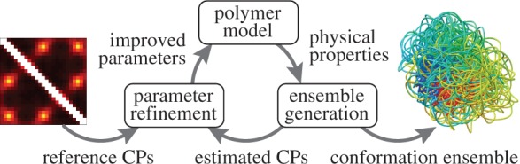
Main components of the proposed computational approach to recover a conformation ensemble from a given set of reference CPs.
Coarse-grained polymer model of chromatin
We assume that chromatin exists as a fiber with an average diameter of 30 nm, and that the conformation of this fiber is determined primarily by its stretching resistance, bending stiffness and excluded volume. To approximate these physical properties, we use a bead-chain model, with each bead representing a chromatin segment of 3–6 kb (34). A similar model was proposed by Rosa et al. (35) and was recently used to simulate the entire genome of budding yeast (36). Following Baù et al. (12), we also assume that the chromatin fiber is subjected to unknown external constraints, e.g. due to looping interactions or confinement, and that the average effects of these constraints can be approximated by additional harmonic restraints connecting particular beads in the chain (Figure 2a).
Figure 2.

Schematic representations of (a) restrained bead-chain polymer model used for BD simulations of a 30-nm chromatin fiber subjected to looping constraints and (b) application of the LMS algorithm to the optimization of the parameters in the general linear model (Equation 9) used to predict restraint spring constants from reference CPs.
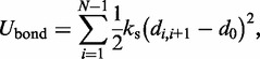
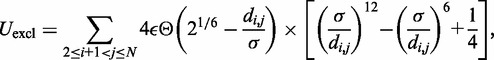
Thus, the potential energy U of the bead chain can be expressed as the sum of four terms,
| (1) |
The first term  accounts for the chain’s resistance to stretching and results from connecting adjacent beads with harmonic springs,
 |
(2) |
where 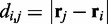 is the distance between beads i and j, N is the number of beads in the chain,
  is the spring constant,
  is the position vector for bead i,
  is the equilibrium bond length and
  = 30 nm is the unit of length used in our simulations (Table 1).
Table 1.
Parameter values used to simulate the restrained bead-chain polymer model of chromatin and to provide a physically realistic approximation of the mechanical properties of chromatin, as currently known from experiments
| Parameter | Symbol | Reduced units | SI units |
|---|---|---|---|
| Thermal energya |  |
1.0 |  |
| Bead massb | m | 1.0 |  |
| Lennard–Jones size parameter |  |
1.0 | 30 nm |
| Lennard–Jones energy parameter |  |
 |
 |
| Bead separation |  |
 |
30 nm |
| Contact distancec |  |
 |
45 nm |
| Bond spring constantd |  |
 |
 |
| Persistence lengthe |  |
 |
120 nm |
| Bending energy constant |  |
 |
 |
| Time step/damping constantf |  |
 |
 |
aEnergy per bead per degree of freedom at T = 300 K.
bRepresentative value based on the experimental measurement of 23.3 MDa for a 15.5-kb fragment of 30-nm chromatin upstream of the chicken  -globin locus (42).
cFollowing Rosa et al. (35), equivalent to assuming that contacts between chromatin fibers are mediated by proteins of 15-nm diameter.
dFrom experiments, the stretching modulus is  5–150 pN (43), hence
  ranges from
  to
to  .
.
eFrom experiments,  30 – 200 nm (43).
fTo maximize conformation sampling efficiency, we used the largest value of  found to maintain stability of the BD simulations. A lower bound for
  can be estimated by considering a chromatin sphere of radius r = 15 nm and using
  with the viscosity of water
  = 890 µPa s at 25°C and 1 bar (44). Then,
  18 ns.
The second potential energy term  accounts for the chain’s resistance to bending and results from subjecting each triplet of adjacent beads to a harmonic bending potential (37),
 |
(3) |
where  is the angle between the displacement vectors
  and
and  is an angular ‘spring constant’,
  is the persistence length of the chain (38),
  is the Boltzmann constant and T is the absolute temperature.
The third potential energy term,  , accounts for the excluded volume, or effective thickness, of the chain and is treated using the repulsive part of the Lennard–Jones potential,
 |
(4) |
where  is the unit of energy in our simulations,
  = 30 nm is the effective thickness of the fiber (Table 1) and
  is the Heaviside step function, which equals 1 when
  and 0 otherwise.
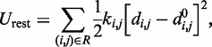
The last potential energy term,  , accounts for the presence of external forces or constraints that affect the shape of the chromatin fiber as well as the probability of contact between different segments of the fiber. In particular, we assume that the average effects of these constraints can be reproduced reasonably well by including a sufficient number of harmonic restraints that connect a subset of the beads in the chain,
 |
(5) |
where R is the set of pairs of beads connected by harmonic restraints and  (
( ) is the spring constant (equilibrium distance) for the restraint connecting beads i and j. The actual members (i, j) of the set R and the corresponding values of
  and
and  are adjustable parameters in this model of restrained chromatin.
Generation of conformation ensembles
To obtain optimal values for these adjustable parameters, we compare a reference set of probabilities of contact between the beads in the chain with a set of corresponding probabilities estimated from an ensemble comprising a large number of bead-chain conformations.
Simulations of bead chain
To obtain such an ensemble, we start by minimizing the potential energy of an initial conformation. To this end, we use the Polak–Ribiere modification of the conjugate gradient algorithm (39). Next, we equilibrate the energy-minimized chain by performing 106 steps of Brownian dynamics (BD) simulation. We then perform an additional BD simulation during which we collect one conformation every 100 integration steps. The set of conformations collected from a single simulation trajectory constitute a conformation ensemble.
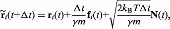
To perform the BD simulations, we apply a second-order algorithm (40,41), which we simplify to neglect the effects of hydrodynamic interactions. Specifically, for each bead i, we calculate a tentative new position at time  using the position
  of the bead and the force
  on the bead at time t,
 |
(6) |
where 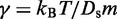 is the damping constant,
  is the self-diffusion coefficient,
  is the integration time step, m is the mass of each bead and N(t) is a random displacement vector whose components are normally distributed with mean 0 and variance 1. Next, we use the tentative bead positions to calculate a tentative new force
  for each bead i. Then, for each bead i, we calculate a more accurate position using the tentative position and tentative force at time
  and the force at time t,
| (7) |
Finally, these latter bead positions are used to calculate more accurate forces  at time
Estimation of CPs
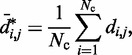
To estimate the bead CPs from an ensemble of bead chain conformations, we analyze each member of the ensemble and check for the occurrence of contacts within all possible pairs of beads in the chain. Following Rosa et al. (35), a contact between two beads is defined to occur whenever the distance between the beads is less than a predefined ‘contact’ distance,  (Table 1). Hence, we estimate the probability of contact
  between beads i and j by calculating the proportion of conformations in which a contact occurs between those beads,
 |
(8) |
where  is the total number of conformations in the ensemble and
  is the distance between beads i and j in conformation l of the ensemble.
Refinement of model parameters
In this work, we assume that a set of reference CPs, denoted  , is available for
  , and the problem is to find an ensemble of bead-chain conformations consistent with those CPs. To this end, we need to optimize the adjustable parameters of the bead-chain model so that simulating such a model yields a conformation ensemble whose estimated CPs
  match as closely as possible the corresponding reference CPs
  for
for  .
.
The adjustable parameters to be optimized are the pairs of indexes  and the values of
  and
and  for each (i, j). To begin to tackle this complex problem, we choose to reduce the number of adjustable parameters by fixing the members (i, j) of the set R at the start of the optimization procedure and by using zero as the equilibrium distance for the harmonic restraints, i.e.
  . Although
  , excluded volume interactions (Equation 4) prevent beads from overlapping.
Placement of harmonic restraints
To determine the pairs  of beads that must be connected by harmonic restraints, we analyze the given set of reference CPs
  , for
, for  , by using a peak detection algorithm. Specifically, we construct a smooth surface z = g(x,y) such that
  for
for  . Each peak on this CP ‘surface’ corresponds to a pair of beads that interact more frequently than their neighbors. Thus, we find the pair of integers (i, j) closest to the location
  of each peak in the CP surface, and we add (i, j) to the set R of pairs of beads connected by harmonic restraints. To find the location
  of each peak, we slice the surface at every point (i,j), for
  , using the four vertical planes x = i, y = j, x + y = i + j and x – y = i – j. Next, we find the local maxima of the curve generated by each slice. If the curves on all four slices have a local maximum close to
  , then we deem
  to be the location of a peak on the CP surface.
Optimization of restraint spring constants
The remaining group of adjustable parameters are the spring constants  that determine the strength of the harmonic restraints on bead pairs
  . To predict these spring constants from the known reference CPs, we use the general linear model
| (9) |
Here, k* is a vector containing n predicted spring constants  of the harmonic restraints, where n is the number of bead pairs in R; W is an
  matrix of model parameters and p* is a vector containing n + 1 elements, where the first n elements are the reference CPs
  for the pairs of beads connected by the n harmonic restraints, and the last element is a non-zero constant c that allows W to map the background CPs of an unrestrained chain to zero spring constants. As c is multiplied by appropriate weights, its value can be arbitrary. To minimize roundoff errors, however, we use
Now the problem of finding optimal values for the spring constants  becomes a problem of determining the optimal elements of the matrix W. This is not a trivial problem, because each spring constant
  may in general affect not only the CP for the pair (i, j) of beads connected by that spring but also the CPs for other pairs of beads in the chain, including those connected by other restraints. Also, because Equation 9 is an approximation, the optimal W will not necessarily yield valid spring constants
  when p* changes. Thus, in general, an optimal W must be determined for each given p*.
One could argue that predicting the  s through Equation 9 is an unnecessary complication, because optimal
  s could be found more simply by using a standard optimization algorithm that adjusts the
  s to minimize the sum of squared differences
  . We did not pursue such a blind approach, however, because we suspected that it would be less efficient than alternative methods that take advantage of additional information about the underlying physical system. Such information, in the proposed approach, is the hypothesis that there exists an ‘inverse’ system that converts the CPs to spring constants according to the general linear model of Equation 9.
To find optimal elements for W in Equation 9, we apply the least mean squares (LMS) algorithm developed by Widrow and colleagues (45–47) (see the Appendix). This simple yet powerful algorithm has been extensively used in the field of adaptive signal processing to optimize a digital filter structure known as adaptive linear combiner (ALC). An ALC performs a dot product between a time-varying weight vector  and a time-varying input vector
  , thus obtaining a scalar output yk = wkTxk, which is required to approximate a given desired signal
  at each discrete time step k. To meet this requirement, the LMS algorithm uses a steepest descent scheme that iteratively adjusts the elements of the weight vector
  at each time step k using
| (10) |
where  is the error at time step k and
  is a gain factor that affects the speed of convergence and the stability of the algorithm.
To apply the LMS algorithm toward the optimization of the parameter matrix W in Equation 9, we allow this matrix, the CPs and the predicted spring constants to vary with iteration index k, i.e. kk = Wkpk. We then treat the elements of  and the rows of
  as the outputs and transposed weight vectors, respectively, of n ALCs,
| (11) |
| (12) |
To complete this application of the LMS algorithm, we must provide appropriate inputs to the ALCs and obtain appropriate errors, which are necessary to adjust the weight vectors. To obtain an input vector  for all ALCs, we first predict a set of restraint spring constants using the parameter matrix available at iteration k and the constant vector of reference CPs (first block in Figure 2b), i.e.
  . Next, we use this set of spring constants to generate, through BD simulations, an ensemble of bead-chain conformations, and we use this ensemble to estimate the CPs for the restrained bead pairs
  (second block in Figure 2b). The resulting vector
  of estimated CPs is now used as input for all n ALCs, which produce a corresponding output vector
  = Wk
= Wk at iteration k (third block in Figure 2b). If the weights of the ALCs were optimal, then the ALC outputs in
  at iteration k would be very close to the spring constants in
  , which were used to generate the ensemble of conformations from which
  was estimated. Therefore, the ALC errors are the elements of the vector εk =
  −
−  , which we can finally use to compute a better estimate of the parameter matrix for the next iteration,
| (13) |
To ensure stability of the LMS algorithm, we need a gain factor  , where tr[R] is the trace of the input correlation matrix (47). Thus, to calculate a safe value for
  we let
  and we use the approximation
| (14) |
where we account for both current and reference CPs in order to decrease  when
when  is large and to bound
  from above when
  is small. To determine the first vector of predicted restraint spring constants
  we assume a linear relationship between each
  and the corresponding reference CP
  . Specifically, we set
  for
for  , where a0 = 2 − 2
 /(
/( −
−  ), a1 = 2/(
 −
−  ) and
) and  (
( ) is the minimum (maximum) value of the reference CPs
  for
for  . This choice yields initial spring constants ranging from 20 to 40% of the maximum value of 10 that we allow
  to take. Then, to begin the restraint optimization procedure with the first vector of estimated CPs
  we set the diagonal elements of
  equal to 1 and all other elements equal to 0.
Selection of optimal ensemble
After a sufficient number of iterations, the restraint optimization procedure described above should yield a set of predicted spring constants  that produce a good match between the CPs estimated for the ‘restrained’ bead pairs and the corresponding reference CPs, i.e.
  for
for  . Our goal, however, is to generate an optimal ensemble of bead-chain conformations such that the CPs estimated for ‘all’ bead pairs, not just the restrained ones, closely match the corresponding reference CPs, i.e. we want
  for
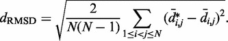
for  . To quantify the goodness of match between estimated and reference CPs, we calculate the root mean-squared deviation (RMSD) between the two sets of probabilities,
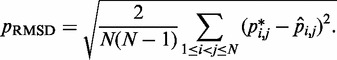 |
(15) |
To find the set of restraint spring constants that minimize  , we perform 40 iterations of the LMS algorithm (Equation 13) during the restraint optimization procedure described above. To accelerate these iterations, we perform only
  steps during the BD simulations from which the CPs are estimated at each iteration. In general, the conformation ensembles produced by such short simulations will depend on the initial bead-chain conformation used for the BD simulations. Therefore, to find the ensemble that minimizes
  , we perform several trials of the restraint optimization procedure. In each trial, we use a different initial conformation for the simulations, and we identify the set of restraint spring constants that minimize
  among all iterations performed. Next, these optimal spring constants and the corresponding initial conformation are used to generate a larger conformation ensemble, this time by performing 108 steps of BD simulation. Among the larger conformation ensembles obtained from all trials, we select the one that yields the smallest
  . This final ensemble is the one we deem to be optimal, i.e. most consistent with the reference CPs.
Generation of initial conformations
To obtain the different initial bead-chain conformations used for each trial of the restraint optimization procedure, one could simply generate a number of random conformations. We choose, however, a more deterministic approach aimed at generating conformations with different relative orientations of loops. Specifically, we design each initial conformation in the shape of a tight cylindrical bundle (Figure 6). To generate the bundle, all the beads connected by harmonic restraints are arranged on a circle whose circumference is just large enough to prevent overlapping those beads. Next, the intervening fragments that contain the other beads of the chain are used to connect the beads on the circle. As they join the beads on the circle, these fragments are forced to run perpendicular to the plane of the circle. Hence, there are two ways in which each fragment can connect two adjacent beads on the circle: on the same side of the plane of the circle, or on opposite sides. By connecting the beads on the circle with the intervening fragments in all possible ways, we can generate up to  distinct conformations, where
  is the number of beads on the circle and where we omit those conformations that result from reflecting other conformations about the plane of the circle. In the present study, we selected up to 32 different bundle conformations to perform the trials of the restraint optimization procedure (Table 2).
Figure 6.
Initial conformations used in eight trials of the ensemble recovery procedure for a chain with 35 beads and 6 restraints (third row in Table 2), shown before (top) and after (bottom) minimization of the potential energy, Equation 1. Images were generated using UCSF Chimera (48).
Table 2.
Validation of the conformation ensemble recovery procedure using reference CPs estimated by simulating test systems of increasing complexity
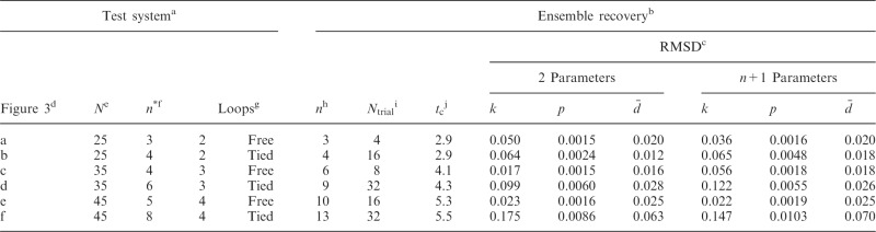 |
aCharacteristics of test systems used to generate conformation ensembles from which reference CPs were estimated.
bResults of ensemble recovery procedure applied to reference CPs.
cRMSD between recovered and reference values of restraint spring constants (k), CPs (p) and mean inter-bead distances ( ), achieved when using a general linear model (Equation 9) with the specified number of parameters per spring constant.
dLabel used to identify test system in Figure 3.
eNumber of beads in the chain.
fNumber of restraints used to induce the loops in the bead chain.
gNumber and type of induced loops.
hNumber of restraints found by peak detection algorithm.
iNumber of trials performed to select the optimal ensemble.
jAverage computation time per trial in hours when performing each trial with n + 1 parameters on one core of a 2.2-GHz AMD Opteron Processor 2427.
RESULTS AND DISCUSSION
Test systems
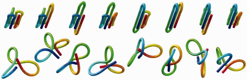
To validate our computational method, we considered six test systems of increasing complexity. Each test system consisted of the same bead-chain model that we used to recover an optimal conformation ensemble from reference CPs. In each such system, however, we induced the formation of specific loops by connecting appropriate beads with up to eight harmonic restraints (Supplementary Table S1). To vary the complexity of these test systems, we varied the number of beads in the chain and the number of induced loops (Table 2). In particular, we simulated chains of 25, 35 and 45 beads with 2, 3 and 4 ‘free’ loops, respectively. To mimic the effects of confinement constraints, we also simulated the same chains with additional restraints connecting the middle beads of free loops across such loops, as shown schematically in Supplementary Table S1, thus giving rise to ‘tied’ loops.
We used the same value of  for the spring constants of all restrained bead pairs (i, j) in all test systems. The conformations of these test systems obtained after minimizing their potential energy are shown in Figure 3.
Figure 3.
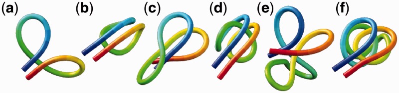
Energy-minimized conformations of the test systems used to generate reference CPs for validating the proposed computational method. The systems are labeled as in Table 2. Images were generated using UCSF Chimera (48).
Reference CPs
To obtain reference sets of estimated bead CPs  , for
, for  , in each of the six test systems, we generated corresponding ensembles of bead-chain conformations by performing BD simulations following the same protocol described above for the ensemble recovery procedure. In particular, for each test system, we constructed an initial bead-chain conformation by threading the appropriate number of beads into the path of a 3D Hilbert curve (21). We then minimized the potential energy of the initial conformation (Figure 3), equilibrated the system with 106 simulation steps and performed 108 additional steps, during which we collected one bead-chain conformation every 100 steps. From the collected conformations, we estimated
  using Equation 8. The CPs estimated for a chain of 45 beads with four free loops and four tied loops are represented as heat maps in Figure 4a. Also highlighted are the locations of bead pairs (i, j) that were connected by harmonic restraints to induce the formation of loops or to tie the loops.
Figure 4.
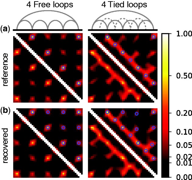
Heat maps representing (a) reference and (b) recovered CPs for a chain of 45 beads with (left) four free loops or (right) four tied loops. Free loops result from connecting loop end-beads with harmonic restraints (gray arcs in top-left schematic), while tied loops result from connecting middle beads across free loops (dotted arcs in top-right schematic). Blue circles on the maps identify pairs of beads that were restrained (a) when generating reference CPs and (b) when performing the ensemble recovery procedure. Test systems with two and three loops (Table 2) yielded a similarly good visual match between reference and recovered CP maps (data not shown).
These heat maps qualitatively confirm the intuition that  for beads connected by restraints and for nearby beads along the chain should be greater than the background CP. These maps, however, also reveal enhanced CPs for pairs of beads that were not directly connected by harmonic restraints and that were relatively distant along the chain from other restrained beads. A similar phenomenon was observed for the chain with 35 beads, but not for the chain with 25 beads (data not shown). Thus, an enhanced probability of contact between two beads in the chain is not always due to an external force directly pulling those beads toward each other. These results underscore the complexity of interactions that can arise even for a chain of only 35 beads, when such a chain is subjected to looping constraints.
Relation between CPs and mean inter-bead distances
Simulating the above test systems to validate our computational method also provided an opportunity to investigate the behavior of chromatin assumed in previous related works. In particular, to infer the 3D conformation of chromatin from experimentally measured CPs, previous studies have assumed that the mean spatial distance d between two DNA fragments can be deduced from their CP p through a simple functional relation. For example, the power law  has been used with exponents
  (27,28) and
  (30). Alternatively, exponential decay (29) and logarithmic types of relations (12) have also been used. To assess whether a simple relationship between mean inter-bead distance,
 |
(16) |
and corresponding CP  does hold for our test systems, we obtained
  from the same conformation ensembles that were used to determine
  .
.
First, however, we analyzed the results from simulations of bead chains that lacked harmonic restraints. A plot of  against
  , for
, for  , obtained from simulating an unrestrained chain of 45 beads, shows that, in the absence of constraints inducing loop formation, the CPs follow a clear trend with a peak at
  (Figure 5a). We observed similar trends for chains with 35 and 25 beads (data not shown).
Figure 5.
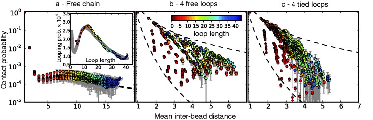
Variation of bead CPs with mean inter-bead distance in reference ensembles for chain (a) without restraints, (b) with four free loops and (c) with four tied loops. Each point represents one of the possible bead pairs in the chain. Error bars are standard deviations over 10 independent simulations. The dashed line in (a) is a fit of the power law  , giving
  . Inset in (a): looping probability versus loop length in ensemble for chain without restraints. The curve in this inset is a fit of Equation 3 from (26). The dashed curves in (b) and (c) are power laws with exponents −8 and −3. Distances are in units of
  .
.
As  does not vary significantly among pairs of beads separated by similar mean spatial distances
  or by similar loop lengths j – i (Figure 5a), it is reasonable to estimate looping probabilities by averaging
  over constant values of j – i (Figure 5a, inset). We found that such looping probabilities for an unrestrained chain of 45 beads approximately follow the trend predicted by theory for worm-like chains with non-zero persistence length and non-zero contact distance (26), thus confirming that our simulations can reproduce the behavior of such chains. Furthermore, noting a monotonic relation between
  and
and  for
for  , we also fitted the power law
  to our simulation data for the unrestrained chain, and we obtained
  , which approximately agrees with the value
  reported in (30). These results suggest that, in the absence of harmonic restraints and for
  sufficiently large, it may be appropriate to assume a simple monotonic relation between
  and
and  and to use such relation for predicting approximate values of
  from known or measured values of
  .
.
We next analyzed the results from the simulations of the test systems, where specific beads were connected by restraints as described above. In this case, the plots of  against
  indicate that the addition of harmonic restraints complicates the relation between
  and
and  (Figure 5b and c) far beyond the clear trend obtained from the simulations of the unrestrained chains. In particular, when harmonic restraints are present, the CPs are overall greater than the corresponding values observed in the absence of restraints, and there appears to exist no simple law that relates
  and
and  . In fact, different pairs of beads separated by similar mean spatial distances or by similar loop lengths yield CPs that differ significantly by up to four orders of magnitude. The observed variation of
  with
with  for the chain with four free loops is bounded by power laws with exponents as different as −3 and −8 (Figure 5b and c, dashed lines). Hence, for the test systems considered in the present study, assuming a simple functional relation and using such relation to calculate
  from
from  would introduce large fractional errors in the predicted values of
  , and those errors would increase with decreasing bead CPs. These results thus motivate the development of computational approaches that do not rely on calculating
  from
from  but directly compare estimated CPs with reference CPs to infer a configuration ensemble.
Method validation
Ensemble recovery from reference CPs
After obtaining the reference set of bead CPs  for each test system, we applied our computational method to recover an ensemble of conformations whose estimated CPs
  match the corresponding reference CPs. We began by selecting a few pairs of beads to be connected with harmonic restraints. This selection was performed in an automated fashion by analyzing the reference CP maps with the peak detection algorithm described above. The algorithm successfully identified all of the bead pairs that were connected by harmonic restraints in the test systems used to generate
  (Supplementary Table S1). Moreover, for chains with 35 and 45 beads, the algorithm found 2, 3 or 5 additional bead pairs that were not restrained in the test systems (Supplementary Table S1) but nevertheless gave rise to CPs enhanced above the background (Figure 4).
We next adjusted the spring constants  of the guessed restraints by performing up to 32 trials of our iterative restraint optimization procedure. Each trial used a different initial chain conformation (Figure 6) to start the BD simulations performed to estimate the CPs for the restrained bead chain.
From each trial, we obtained a different set of restraint spring constants together with the corresponding ensemble of chain conformations. For each such conformation ensemble, we used Equation 15 to calculate  , the RMSD between the CPs
  estimated for that ensemble and the corresponding reference CPs
  previously obtained for the test system under study. We found that
  varies among the trials of the ensemble recovery procedure for a given test system and that this variation increases with the complexity of the test system (Figure 7), indicating that, within the simulated time intervals, the restrained bead chain tends to get trapped into local energy minima that depend on the initial chain conformation.
Figure 7.
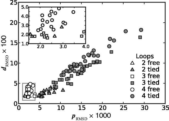
Plots of RMSD of mean inter-bead distances (Equation 17) against RMSD of CPs (Equation 15) for all trials of the ensemble recovery procedure and for all tested systems. Each point represents RMSD values obtained from an ensemble of 106 conformations at the end of a particular trial. Inset: enlarged view of boxed area. Distances are in units of  .
.
For each recovered conformation ensemble, we also calculated the mean inter-bead distances  for
for  . Then, to compare quantitatively these mean inter-bead distances with the corresponding reference quantities
  we calculated the RMSD between the two sets of distances (30),
 |
(17) |
We found that minimizing  over the trials for a given test system yields the smallest, or a relatively small value for the RMSD of the mean inter-bead distances,
  (Figure 7). These results indicate that minimizing
  relative to a set of reference CPs
  is an effective strategy for identifying a conformation ensemble that closely matches the mean inter-bead distances of the original conformation ensemble from which the
  were estimated or measured.
Therefore, to conclude our ensemble recovery procedure, for each test system, we selected the set of restraint spring constants and the corresponding conformation ensemble that minimized  among all trials. Comparing the heat maps of the CPs estimated from recovered and reference ensembles for chains with 45 beads (Figure 4a and b) shows a good qualitative agreement between the two ensembles. A similar good agreement was also observed for the simpler test systems (data not shown). This agreement is also apparent in plots of
  against
  (Figure 8a).
Figure 8.
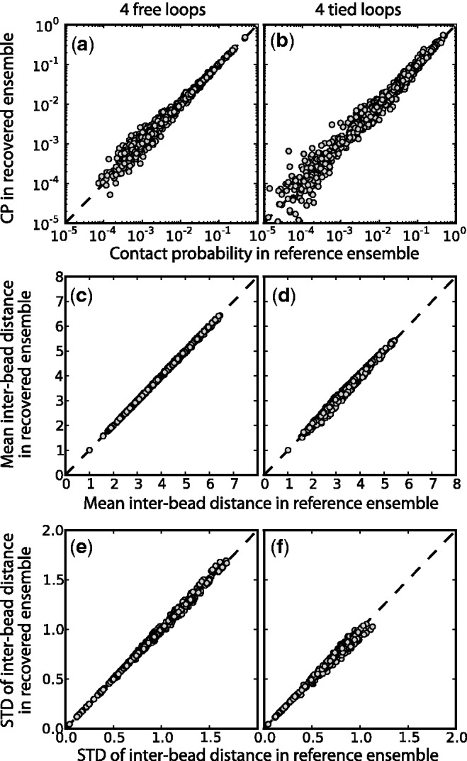
Comparison of (a,b) bead CPs, (c,d) mean inter-bead distances and (e,f) standard deviation of inter-bead distance determined from optimal recovered ensemble to respective quantities determined from reference ensemble for a chain with 45 beads and (a,c,e) 4 free loops or (b,d,f) 4 tied loops. Each point represents one of the possible bead pairs in the chain. The dashed lines are plots of y = x, not linear fits. Distances are in units of  . Better correlations were observed for test systems with three and two loops (data not shown).
Furthermore, the mean and standard deviation of the inter-bead distances in the recovered conformation ensembles are in excellent agreement with the corresponding quantities calculated for the reference ensembles (Figure 8b and c), confirming that our procedure successfully recovered not only the average frequency of the various inter-bead interactions but also the average inter-bead distances and the extent to which these distances fluctuate about the mean.
To visualize the reference and recovered conformation ensembles, we uniformly extracted 100 conformations from each such ensemble and aligned those conformations on the beads that were restrained in the test system used to generated the reference ensemble. The resulting 3D representations of the reference and recovered conformation ensembles reveal large fluctuations in the positions of the loops (Figure 9). The same regions of space, however, tend to be occupied by corresponding loops in the reference and recovered ensembles, thus providing a visual confirmation of the similarity between the average spatial arrangements of the two ensembles.
Figure 9.

Spatial representation of reference (left) and recovered (right) conformation ensembles for bead chains of 45 beads with (a) four free loops and (b) four tied loops. Each depicted ensemble consists of 100 conformations extracted at equal intervals from 108 steps of BD simulation and aligned on the beads that were connected by harmonic restraints in the simulations used to generate the reference ensembles. The coloring order along each chain is red, yellow, green, cyan and blue. Images were generated using UCSF Chimera (48).
Simplified general linear model
The good agreement that we observed between recovered and reference ensembles is in fact a consequence of successfully optimizing the general linear model of Equation 9 with the LMS algorithm. This optimization resulted in a good prediction of restraint spring constants from the reference CPs associated with the restrained bead pairs. In fact, as noted above, some bead pairs were chosen by the peak detection algorithm for restraining, even though they were not restrained in the test systems. During the ensemble recovery procedure, however, the spring constants for the restraints on these bead pairs decreased to small values relative to the spring constants restraining the other bead pairs (Supplementary Table S1). These results indicate that the ensemble recovery procedure correctly distinguished the pairs of beads that were directly connected by harmonic restraints in the reference conformation ensemble from those pairs that were not. In particular, the RMSD,
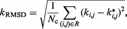 |
(18) |
between the spring constants  predicted during the ensemble recovery procedure and the corresponding value
  used for the restraints in the test systems was <6% of
  for all such systems (Table 2). Thus, the procedure successfully deduced approximate values of the underlying spring constants using only the knowledge of reference CPs.
We asked whether a similarly good prediction of each restraint spring constant could be achieved with fewer than n + 1 non-zero elements per row in the matrix W in Equation 9, i.e. with fewer than n + 1 parameters per spring constant. To answer this question, we repeated the ensemble recovery procedure on all test systems, this time forcing all of the off-diagonal elements of W—except those in the last column—to be zero, thus effectively using only two parameters to predict each spring constant. This choice corresponds to assuming that each restraint spring constant  is linearly related only to the CP
  estimated for the bead pair (i, j) restrained by that spring constant, i.e. ki,j = wi,j
 + ci,j. We found that the resulting RMSDs of the spring constants, CPs and mean inter-bead distances did not differ appreciably from the corresponding values obtained by using n + 1 parameters per spring constant (Table 2). Therefore, for the test systems considered in this study, it appears that the CP associated with each restrained bead pair depends primarily on the spring constant restraining that bead pair. This conclusion, however, may not hold for more complex systems, where the restraints might be less uniformly distributed among the beads and might have more variable spring constants than the restraints we used in this study to generate the reference CPs. For more complex systems, using all parameters in the general linear model of Equation 9 may be necessary to achieve adequate accuracy in the prediction of spring constants from CPs.
Computation time
The majority of the computation time required by the proposed ensemble recovery procedure is consumed by the BD simulations. These simulations are needed to estimate the CPs either for adjusting the spring constants through the LMS algorithm or for selecting the optimal conformation ensemble through a comparison of  values among the ensembles obtained from different initial conformations. The simulations must be sufficiently long to ensure that the variance of the CPs estimated using Equation 8 does not outweigh the variation in CP due to differences in spring constants and initial conformations. In our work with the test systems, obtaining CPs sufficiently precise to ensure rapid convergence of the LMS algorithm in all trials of the restraint optimization procedure required
  steps per simulation. On the other hand, ensuring that the optimal ensemble selected from several trials of the procedure matches the diversity of conformations present in the corresponding reference ensemble required 108 simulation steps, i.e. the same number that was used to obtain each reference ensemble. The average computation time per trial was found to increase linearly with the number of beads (Table 2).
CONCLUSION
We have developed a computational approach to recover chromatin conformation ensembles from a set of reference CPs. The overall strategy of this approach consists of comparing the given set of reference CPs to a set of CPs obtained from simulations of a restrained bead-chain polymer model of chromatin. The results of this comparison are used iteratively to adjust the parameters of the polymer model so that, after a sufficient number of iterations and trials, an optimal conformation ensemble is obtained whose CPs closely match the corresponding reference probabilities. We have validated this procedure by using reference data sets obtained from simulations of six test systems of increasing complexity. For all such systems, the procedure yielded a conformation ensemble whose CPs, mean inter-bead distances and standard deviation of inter-bead distances all agree very closely with the corresponding reference quantities. The most complex test system that we considered was a chain of 45 beads, equivalent to roughly 135–270 kb, containing four tied loops (Figure 3f). Although this system is much smaller than the genomic loci typically investigated in 3C-based experiments, it does provide initial support to the validity of the proposed computational approach, which can already be used to investigate the spatial organization of small genomic regions.
To enable efficient and accurate analysis of experimental data sets obtained from large genomic loci, entire chromosomes or even entire genomes, the proposed computational approach will require additional improvement and validation. For example, whereas the present approach estimates CPs for beads representing fragments of equal lengths, 3C-based experiments typically provide reference CPs for fragments of various lengths. This mismatch could be overcome by mapping the experimental fragments onto the bead-chain contour and by estimating CPs for pairs of mapped fragments, rather than for pairs of beads. Another issue is computational effort. Although the procedure we described lends itself to parallelization, with each trial executing on a separate processor core, it may nevertheless become too demanding for large genomic loci. Computational effort could be lowered by improving the efficiency of conformation sampling, for example through Monte Carlo simulations, and by avoiding Equation 8 in the estimation of CPs, for example by inferring inter-bead distance distributions from sample means and higher moments of  . Finally, further validation of the procedure will require not only the simulation of larger and more complex test systems but also the availability of experimental data sets that include both 3C and FISH measurements on the same genomic region. Applications of our method to the analysis of experimental data and to the study of specific phenomena, such as gene clustering (31), are important issues that will be addressed in the future.
SUPPLEMENTARY DATA
Supplementary Data are available at NAR Online: Supplementary Table 1.
FUNDING
American Cancer Society [Instructional Research 70-002 provided to G.A. through the Moores Cancer Center, University of California, San Diego] and ARCS Foundation, San Diego Chapter [scholarship to D.M.]. Funding for open access charge: American Cancer Society.
Conflict of interest statement. None declared.
Supplementary Material
APPENDIX
THE LMS ALGORITHM
The LMS algorithm (45,46) has found numerous applications in the field of adaptive signal processing, including adaptive system identification, adaptive inverse modeling, adaptive control and adaptive interference canceling (47). This algorithm was developed to optimize iteratively and dynamically the weights of a digital filter structure, known as ALC, that performs the dot product yk = wkTxk, where  is the ALC output,
  is a vector containing n + 1 adjustable weights,
  is a vector containing n + 1 inputs and k is the current time step for the inputs, weights and output. The choice of the inputs in
  and the role of the output
  depend on the specific application of the ALC. All applications, however, include a desired signal
  and require the adjustment of
  at each time step k so that the output
  is, on average, as close as possible to
  or, equivalently, so that the magnitude of the error
| (A1) |
averaged over a long interval of k, is as small as possible. The degree to which the ALC meets this requirement can be quantified, as a function of  , by defining the quadratic performance surface χ = E[εk2], where the expected value
  is taken over the time step k. Hence, the requirement to achieve optimality of the ALC is that the weight vector
  be adjusted at each time step k to minimize
  . The LMS algorithm addresses this requirement by using a variant of the steepest descent algorithm. This variant replaces the gradient
  of the quadratic performance surface with a simpler estimate obtained at time step k directly from
  , i.e.
| (A2) |
where  is the gradient operator with respect to the components of the weight vector
  . The gradient estimate
  is then used to calculate an improved weight vector from the current one,
| (A3) |
where  is a gain factor that determines the size of the step along the negative gradient estimate. A small value of
  causes slow convergence, whereas too large a value of
  causes instability of the algorithm. It has been shown (47) that the LMS algorithm is stable for
  , where
  is the input correlation matrix. The strengths of the LMS algorithm are its simplicity, robustness and relatively rapid convergence despite the presence of noise in the input
  and desired signal
  .
.
REFERENCES
- 1.Felsenfeld G, Groudine M. Controlling the double helix. Nature. 2003;421:448–453. doi: 10.1038/nature01411. [DOI] [PubMed] [Google Scholar]
- 2.Blackwood EM, Kadonaga JT. Going the distance: a current view of enhancer action. Science. 1998;281:60–63. doi: 10.1126/science.281.5373.60. [DOI] [PubMed] [Google Scholar]
- 3.Adhya S. Multipartite genetic control elements: communication by DNA loop. Annu. Rev. Genet. 1989;23:227–250. doi: 10.1146/annurev.ge.23.120189.001303. [DOI] [PubMed] [Google Scholar]
- 4.Carter D, Chakalova L, Osborne CS, Dai Yf, Fraser P. Long-range chromatin regulatory interactions in vivo. Nat. Genet. 2002;32:623–626. doi: 10.1038/ng1051. [DOI] [PubMed] [Google Scholar]
- 5.Schleif R. DNA looping. Annu. Rev. Biochem. 1992;61:199–223. doi: 10.1146/annurev.bi.61.070192.001215. [DOI] [PubMed] [Google Scholar]
- 6.Gheldof N, Tabuchi TM, Dekker J. The active FMR1 promoter is associated with a large domain of altered chromatin conformation with embedded local histone modifications. Proc. Natl Acad. Sci. USA. 2006;103:12463–12468. doi: 10.1073/pnas.0605343103. [DOI] [PMC free article] [PubMed] [Google Scholar]
- 7.Janicki SM, Tsukamoto T, Salghetti SE, Tansey WP, Sachidanandam R, Prasanth KV, Ried T, Shav-Tal Y, Bertrand E, Singer RH, et al. From silencing to gene expression: real-time analysis in single cells. Cell. 2004;116:683–698. doi: 10.1016/s0092-8674(04)00171-0. [DOI] [PMC free article] [PubMed] [Google Scholar]
- 8.Müller WG, Walker D, Hager GL, McNally JG. Large-scale chromatin decondensation and recondensation regulated by transcription from a natural promoter. J. Cell Biol. 2001;154:33–48. doi: 10.1083/jcb.200011069. [DOI] [PMC free article] [PubMed] [Google Scholar]
- 9.Tumbar T, Sudlow G, Belmont AS. Large-scale chromatin unfolding and remodeling induced by VP16 acidic activation domain. J. Cell Biol. 1999;145:1341–1354. doi: 10.1083/jcb.145.7.1341. [DOI] [PMC free article] [PubMed] [Google Scholar]
- 10.Cook PR. The organization of replication and transcription. Science. 1999;284:1790–1795. doi: 10.1126/science.284.5421.1790. [DOI] [PubMed] [Google Scholar]
- 11.Parada LA, Misteli T. Chromosome positioning in the interphase nucleus. Trends Cell Biol. 2002;12:425–432. doi: 10.1016/s0962-8924(02)02351-6. [DOI] [PubMed] [Google Scholar]
- 12.Baù D, Sanyal A, Lajoie BR, Capriotti E, Byron M, Lawrence JB, Dekker J, Marti-Renom MA. The three-dimensional folding of the α-globin gene domain reveals formation of chromatin globules. Nat. Struct. Mol. Biol. 2011;18:107–114. doi: 10.1038/nsmb.1936. [DOI] [PMC free article] [PubMed] [Google Scholar]
- 13.Lucas JS, Bossen C, Murre C. Transcription and recombination factories: common features? Curr. Opin. Cell Biol. 2011;23:318–324. doi: 10.1016/j.ceb.2010.11.007. [DOI] [PMC free article] [PubMed] [Google Scholar]
- 14.Cremer T, Cremer C. Chromosome territories, nuclear architecture and gene regulation in mammalian cells. Nat. Rev. Genet. 2001;2:292–301. doi: 10.1038/35066075. [DOI] [PubMed] [Google Scholar]
- 15.Levsky JM, Singer RH. Fluorescence in situ hybridization: past, present and future. J. Cell Sci. 2003;116:2833–2838. doi: 10.1242/jcs.00633. [DOI] [PubMed] [Google Scholar]
- 16.Huang B, Babcock H, Zhuang X. Breaking the diffraction barrier: super-resolution imaging of cells. Cell. 2010;143:1047–1058. doi: 10.1016/j.cell.2010.12.002. [DOI] [PMC free article] [PubMed] [Google Scholar]
- 17.Zhao Z, Tavoosidana G, Sjolinder M, Gondor A, Mariano P, Wang S, Kanduri C, Lezcano M, Singh Sandhu K, Singh U, et al. Circular chromosome conformation capture (4C) uncovers extensive networks of epigenetically regulated intra- and interchromosomal interactions. Nat. Genet. 2006;38:1341–1347. doi: 10.1038/ng1891. [DOI] [PubMed] [Google Scholar]
- 18.Simonis M, Klous P, Splinter E, Moshkin Y, Willemsen R, de Wit E, van Steensel B, de Laat W. Nuclear organization of active and inactive chromatin domains uncovered by chromosome conformation capture-on-chip (4C) Nat. Genet. 2006;38:1348–1354. doi: 10.1038/ng1896. [DOI] [PubMed] [Google Scholar]
- 19.Dostie J, Richmond TA, Arnaout RA, Selzer RR, Lee WL, Honan TA, Rubio ED, Krumm A, Lamb J, Nusbaum C, et al. Chromosome conformation capture carbon copy (5C): a massively parallel solution for mapping interactions between genomic elements. Genome Res. 2006;16:1299–1309. doi: 10.1101/gr.5571506. [DOI] [PMC free article] [PubMed] [Google Scholar]
- 20.Rodley CDM, Bertels F, Jones B, O’Sullivan JM. Global identification of yeast chromosome interactions using genome conformation capture. Fungal Genet. Biol. 2009;46:879–886. doi: 10.1016/j.fgb.2009.07.006. [DOI] [PubMed] [Google Scholar]
- 21.Lieberman-Aiden E, van Berkum NL, Williams L, Imakaev M, Ragoczy T, Telling A, Amit I, Lajoie BR, Sabo PJ, Dorschner MO, et al. Comprehensive mapping of long-range interactions reveals folding principles of the human genome. Science. 2009;326:289–293. doi: 10.1126/science.1181369. [DOI] [PMC free article] [PubMed] [Google Scholar]
- 22.Dekker J, Rippe K, Dekker M, Kleckner N. Capturing chromosome conformation. Science. 2002;295:1306–1311. doi: 10.1126/science.1067799. [DOI] [PubMed] [Google Scholar]
- 23.de Wit E, de Laat W. A decade of 3C technologies: insights into nuclear organization. Genes Dev. 2012;26:11–24. doi: 10.1101/gad.179804.111. [DOI] [PMC free article] [PubMed] [Google Scholar]
- 24.Iyer B, Kenward M, Arya G. Hierarchies in eukaryotic genome organization: insights from polymer theory and simulations. BMC Biophys. 2011;4:8. doi: 10.1186/2046-1682-4-8. [DOI] [PMC free article] [PubMed] [Google Scholar]
- 25.Marti-Renom MA, Mirny LA. Bridging the resolution gap in structural modeling of 3D genome organization. PLoS Comput. Biol. 2011;7:e1002125. doi: 10.1371/journal.pcbi.1002125. [DOI] [PMC free article] [PubMed] [Google Scholar]
- 26.Rippe K. Making contacts on a nucleic acid polymer. Trends Biochem. Sci. 2001;26:, 733–740. doi: 10.1016/s0968-0004(01)01978-8. [DOI] [PubMed] [Google Scholar]
- 27.Fraser J, Rousseau M, Shenker S, Ferraiuolo M, Hayashizaki Y, Blanchette M, Dostie J. Chromatin conformation signatures of cellular differentiation. Genome Biol. 2009;10:R37. doi: 10.1186/gb-2009-10-4-r37. [DOI] [PMC free article] [PubMed] [Google Scholar]
- 28.Duan Z, Andronescu M, Schutz K, McIlwain S, Kim YJ, Lee C, Shendure J, Fields S, Blau CA, Noble WS. A three-dimensional model of the yeast genome. Nature. 2010;465:363–367. doi: 10.1038/nature08973. [DOI] [PMC free article] [PubMed] [Google Scholar]
- 29.Tanizawa H, Iwasaki O, Tanaka A, Capizzi JR, Wickramasinghe P, Lee M, Fu Z, Noma K. Mapping of long-range associations throughout the fission yeast genome reveals global genome organization linked to transcriptional regulation. Nucleic Acids Res. 2010;38:8164–8177. doi: 10.1093/nar/gkq955. [DOI] [PMC free article] [PubMed] [Google Scholar]
- 30.Rousseau M, Fraser J, Ferraiuolo M, Dostie J, Blanchette M. Three-dimensional modeling of chromatin structure from interaction frequency data using Markov chain Monte Carlo sampling. BMC Bioinformatics. 2011;12:414. doi: 10.1186/1471-2105-12-414. [DOI] [PMC free article] [PubMed] [Google Scholar]
- 31.Gehlen LR, Gruenert G, Jones MB, Rodley CD, Langowski J, O’Sullivan JM. Chromosome positioning and the clustering of functionally related loci in yeast is driven by chromosomal interactions. Nucleus. 2012;3:370–383. doi: 10.4161/nucl.20971. [DOI] [PubMed] [Google Scholar]
- 32.de Gennes PG. Scaling Concepts in Polymer Physics. New York: Cornell University Press; 1979. [Google Scholar]
- 33.Shimada J, Yamakawa H. Ring-closure probabilities for twisted wormlike chains. Application to DNA. Macromolecules. 1984;17:689–698. [Google Scholar]
- 34.Robinson PJJ, Fairall L, Huynh VAT, Rhodes D. EM measurements define the dimensions of the “30-nm” chromatin fiber: evidence for a compact, interdigitated structure. Proc. Natl Acad. Sci. USA. 2006;103:6506–6511. doi: 10.1073/pnas.0601212103. [DOI] [PMC free article] [PubMed] [Google Scholar]
- 35.Rosa A, Becker NB, Everaers R. Looping probabilities in model interphase chromosomes. Biophys. J. 2010;98:2410–2419. doi: 10.1016/j.bpj.2010.01.054. [DOI] [PMC free article] [PubMed] [Google Scholar]
- 36.Tokuda N, Terada TP, Sasai M. Dynamical modeling of three-dimensional genome organization in interphase budding yeast. Biophys. J. 2012;102:296–304. doi: 10.1016/j.bpj.2011.12.005. [DOI] [PMC free article] [PubMed] [Google Scholar]
- 37.Allen MP, Tildesley DJ. Computer Simulation of Liquids. New York: Oxford University Press; 1987. [Google Scholar]
- 38.Langowski J, Heermann DW. Computational modeling of the chromatin fiber. Semin. Cell Dev. Biol. 2007;18:659–667. doi: 10.1016/j.semcdb.2007.08.011. [DOI] [PubMed] [Google Scholar]
- 39.Press WH, Teukolsky SA, Vetterling WT, Flannery BP. Numerical Recipes in C. 2nd edn. Cambridge, UK: Cambridge University Press; 1992. [Google Scholar]
- 40.Iniesta A, de la Torre JG. A second-order algorithm for the simulation of the Brownian dynamics of macromolecular models. J. Chem. Phys. 1990;92:2015–2018. [Google Scholar]
- 41.Klenin K, Merlitz H, Langowski J. A Brownian dynamics program for the simulation of linear and circular DNA and other wormlike chain polyelectrolytes. Biophys. J. 1998;74:780–788. doi: 10.1016/S0006-3495(98)74003-2. [DOI] [PMC free article] [PubMed] [Google Scholar]
- 42.Ghirlando R, Litt MD, Prioleau MN, Recillas-Targa F, Felsenfeld G. Physical properties of a genomic condensed chromatin fragment. J. Mol. Biol. 2004;336:597–605. doi: 10.1016/j.jmb.2003.12.049. [DOI] [PubMed] [Google Scholar]
- 43.Lavelle C. Forces and torques in the nucleus: chromatin under mechanical constraints. Biochem. Cell Biol. 2009;87:307–322. doi: 10.1139/O08-123. [DOI] [PubMed] [Google Scholar]
- 44.Haynes WM, editor. CRC Handbook of Chemistry and Physics. 92nd edn. Boca Raton, FL, USA: CRC Press; 2011. [Google Scholar]
- 45.Widrow B, Glover JRJ, McCool J, Kaunitz J, Williams C, Hearn R, Zeidler J, Eugene Dong J, Goodlin R. Adaptive noise cancelling: principles and applications. Proceedings of the IEEE. 1975;Vol 63:1692–1716. [Google Scholar]
- 46.Widrow B. Adaptive filters. In: Kalman RE, De Claris N, editors. Aspects of Network and System Theory. New York: Holt, Rinehart and Winston; 1970. pp. 503–587. [Google Scholar]
- 47.Widrow B, Stearns SD. Adaptive Signal Processing. Englewood Cliffs, NJ: Prentice Hall; 1985. [Google Scholar]
- 48.Pettersen EF, Goddard TD, Huang CC, Couch GS, Greenblatt DM, Meng EC, Ferrin TE. UCSF chimera—a visualization system for exploratory research and analysis. J. Comput. Chem. 2004;25:1605–1612. doi: 10.1002/jcc.20084. [DOI] [PubMed] [Google Scholar]
Associated Data
This section collects any data citations, data availability statements, or supplementary materials included in this article.