DataView: A Tutorial Tool for Data Analysis. Template-based Spike Sorting and Frequency Analysis.

Abstract

DataView is a Windows program for viewing and analyzing digital data derived from analog signals using A/D acquisition systems. It is primarily designed for research neuroscientists, but its low (or zero) cost makes it a suitable tool for giving students hands-on experience of analysis techniques. It is supplied with many examples of pre-recorded data and also has facilities to allow tutors to use their own - or indeed their students’ - experimental results as the dataset for analysis. This article illustrates the use of DataView with a brief tutorial on template-based spike sorting and frequency analysis. The DataView manual contains detailed instructions and sample datasets for a wide range of other analytical and data-manipulation techniques.

Virtually all modern electrophysiological experiments involve the acquisition, display and analysis of digitized data. Typically, fluctuating voltages or currents from intracellular, patch or extracellular recordings are sampled at regular intervals, and stored as digital representations of their values by a data acquisition system incorporating an analogue-to-digital (AD) converter. Many students will be exposed to this to some degree in practical laboratory classes and they will also encounter it in their studies of the primary research literature. However, license and cost conditions usually preclude students installing commercial acquisition systems on their own computers, and indeed, the same conditions often prevent the widespread installation of such systems on open-access university computers. Therefore, it is difficult for students to gain hands-on experience of these processes or to carry out homework exercises outside of scheduled laboratory time. For many students the procedures are simply a “black-box,” which produces hopefully meaningful output when a set of recipes is followed.

The purpose of this report is to introduce DataView as a software tool that can aid in undergraduate and post-graduate training in electrophysiological data analysis. It enables students both to investigate some of the principals of the analysis and manipulation of digital data and to carry out their own investigations using data files from real experiments provided by their instructor or as sample files included with the DataView package. The broad pedagogic aim of such exercises is to enhance the problem-solving capabilities of students. As an example of using DataView in a tutorial context this article describes some exercises to explore the response characteristics of the caudal photoreceptor (CPR) of crayfish.

Many species of macruran decapod crustaceans, including fresh-water crayfish, have a bilateral pair of photo-sensitive mechanosensory integrating interneurones located in their terminal abdominal ganglion (Prosser, 1934; Welsh, 1934; Wilkens and Larimer, 1976). These interneurons have ascending axons whose spikes can be recorded extracellularly with simple bipolar hook electrodes placed on the ventral nerve cord (VNC) rostral to the terminal ganglion. Thus, the preparation is suitable for use in an undergraduate laboratory investigating phenomena such as sensory adaptation, the dynamic and tonic phases of sensory responses, the spectral sensitivity of photoreceptors, or the influence of neuromodulators or drugs on a defined sensory system.

The photoresponse is readily observed as an increase in spike frequency in the extracellular recording (and is even more apparent if the signal is listened to through an audio amplifier). However, the axons of the CPR are quite small, and the CPR spikes are rarely the largest in the mixture of signals recorded from the VNC. It is, therefore, hard to analyse the CPR response quantitatively by hand. DataView has a variety of spike-sorting routines that can help to solve this problem, including principle component analysis and/or wavelet analysis of spike shapes (see Lewicki, 1998 for a review of spike sorting methodologies). However, the most straightforward technique, and one that is well-suited to undergraduate teaching, is to use template-based spike recognition to identify the waveform of the CPR spikes from within the mixture of waveforms contained in the extracellular recording. The response characteristics of the CPR can then be visualized with a plot of the instantaneous spike frequency against time. This article gives step-by-step instructions for achieving this goal with DataView.

DataView is available as described in the Materials and Methods section below.

MATERIALS AND METHODS

Preparation

Adult crayfish (Pacifastacus leniusculus) were obtained from commercial suppliers (Tincleton Koi, Dorset, UK). Crayfish of either sex were anaesthetized by chilling in iced water until immobile, and then the cephalothorax was separated from the abdomen and destroyed. The dorsal abdominal cuticle was removed, along with the extensor muscle. The main blocks of fast flexor muscle were separated into left and right components by a longitudinal cut along the midline, revealing the VNC. The flexor muscle was then removed, after sectioning the 3^rd roots of the abdominal ganglia. The first and second roots of each ganglia were cut, and the entire VNC was dissected free from the ventral abdominal tray, pinned out in a Petri dish lined with Sylgard (Dow Corning), and covered with saline (Van Harreveld, 1936). The VNC was then hemi-sectioned between the fifth and sixth (terminal) abdominal ganglia, so that only one of the bilateral pair of caudal photoreceptor axons was intact in more anterior segments.

Stimulating and Recording

Any white or blue-green light source can be used to stimulate the CPR, although in these experiments the stimulus was delivered from a standard fibre-optic dissecting lamp with a halogen bulb, through a solenoid-controlled shutter. No attempt was made to quantify the intensity or spectral components of the light.

CPR activity was recorded with bipolar hook electrodes placed on the VNC between the fourth and fifth abdominal ganglia and insulated from the saline with Vaseline. The signal from the electrodes was amplified with a standard differential extracellular amplifier (AM Systems) and recorded with a Micro-1401 data acquisition system running Spike 2 software (Cambridge Electronic Design, UK). The solenoid controlling the light stimulus was driven through a relay activated by the analog output of the Micro-1401 system.

Software

DataView is available for download from: http://www.st-andrews.ac.uk/∼wjh/dataview/download.html. Even if the reader already has DataView v5.2.2 installed, this should be un-installed (from the Control Panel) and a new download should be initiated in order to include the sample file used in this tutorial.

The additional program Klustawin can be downloaded and installed from the same web page. This is not needed for the procedures described in this tutorial, but it is needed for several of the analysis routines described in the DataView manual. Klustawin implements a Windows interface for the Unix program KlustaKwik, developed by Ken Harris (2000–2002). These clustering programs are released under the GNU license and their source code can be downloaded by following the links on the page above.

TUTORIAL

The instructions in this section take the user through a sequence of steps in template-based spike recognition and frequency analysis, according to the following outline.

1. Load the data file.

2. Survey the general characteristics of the data.

3. Zoom in on some individual spikes.

4. Select a single spike as a putative example of the class of spikes of interest (the CPR in this case), and form a template from it.

5. Use template recognition to search for all spikes whose shapes match the template within a specified allowed error.

6. View the instantaneous frequency characteristics of the recognized spikes.

7. If appropriate, refine the allowed error to reduce false positives identified by unrealistically high instantaneous frequencies.

8. Examine the frequency characteristics of the recognized spikes to determine whether an appropriate template was chosen (i.e. determine whether the recognized spikes show a stimulus response appropriate for the CPR).

9. If the outcome of (8) is unsatisfactory, repeat from (4) selecting a different spike as the template base.

10. Use the waveform average of recognized spikes to improve the template.

11. Use the instantaneous frequency information to identify frequency outliers indicating false positive or negative recognition, and edit if desired.

12. View the averaged CPR spike shape and compare it to non-CPR spikes.

Load, View, Listen to, and Navigate Files

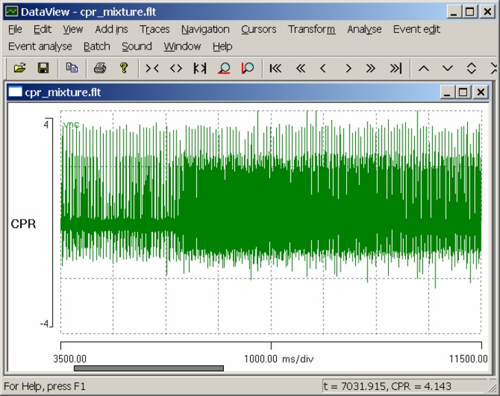
Start DataView and load the file cpr mixture.flt. The flt file name extension shows that the file is in the native DataView floating-point format, while the name itself merely indicates that the file contains a mixed recording of CPR and other spikes. The display shows an eight-second segment of a recording from the dark-adapted VNC, with a light stimulus applied for five seconds, starting 1.5 s into the display (Fig. 1).

Figure 1.

A screen shot of DataView displaying the response of the crayfish ventral nerve cord, including the caudal photoreceptor, to a light stimulus.

There is an obvious increase in spike frequency at about t = 5.8 s (if you hover the mouse over the relevant part of the display you can read the time and voltage from the status bar at the bottom-right of the main window). Select the Sound: Play menu command, and, if you have a sound-enabled computer, you will hear the waveform played as if it were an audio file. Select the Navigation: Show all menu command (or click the Show all toolbar icon), and the whole record is now displayed. Observe that the increased frequency of the photoresponse declines in intensity after the light stimulus terminates (at t = 10 s), but still long outlasts the stimulus.

We now want to find a spike from within the record which we think might be a CPR spike, and whose waveform would thus act as a suitable template for finding other CPR spikes. This is necessarily a trial-and-error process, but the facilities in DataView make it fairly intuitive and easy. First, select the Window: New Window menu command and observe that a duplicate window containing the same data is produced. Select Window: Tile to show the two displays together. We will use the second window to find individual spikes, while maintaining an overview of the whole record in the first window. If we were doing this “for real,” we would use the various zoom tools (on the Navigation menu or the toolbar) to locate candidate spikes; but for the purposes of this tutorial we will use pre-selected spikes.

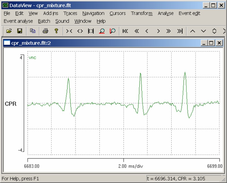
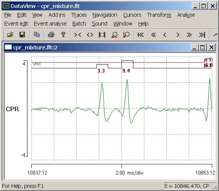
Edit the start time (left-hand end of the timebase axis) to read 6683 ms by double-clicking on the currently-displayed start time (0.00) to select it, typing in 6683 to replace the selection, and pressing the Tab key. Note that whenever you edit a value in DataView the program only updates the value internally when you move the focus away from the value that you edited: this is most easily accomplished by pressing the Tab key after editing. When you Tab away from the start time, the focus shifts to the timebase itself (located at the mid-point scale of the timebase axis). Edit this value to read 2 ms/div (do not forget to Tab away). You should now see three spikes in the display (Fig. 2).

Figure 2.

An expanded view showing three spikes which are potential candidates as templates for use in CPR spike recognition. The window showing the whole record has been minimized.

The spikes are similar in shape, but not identical to each other. We will check out these spikes as potential templates for the CPR spike.

Using Templates for Spike Recognition

We will start by trying the middle spike as a template. Use the Cursors: Place at time menu command to place cursors at 6692 and 6693 ms. This should place a pair of cursors in positions which bracket the middle spike. Note, that the cursors can be dragged with the mouse to adjust their individual positions if desired. The time locations of the cursors are written on screen, but may not exactly match the placement times, since they will only be accurate to the nearest pixel. Now select the Event edit: Template recognition menu command to display the Template recognition dialog box. This is non-modal, which means that you can switch to other parts of the program without dismissing it.

The first thing to do is to tell the program to use the spike between the cursors as a template. The default values for the Data trace (trace 1) and Definition cursor IDs (1 and 2) are correct, so click the Capture button. The waveform between the cursors appears in the window at the top-right of the dialog box. You are now ready to search the record for waveforms that match this captured template. The closeness of match required is set by the Allowed error parameter. The error is a measure of the normalised absolute deviation of the waveform from the template. Now click the Analyse button. After a brief interval, the Event count (near the bottom-left of the dialog box) should show 1491 (or something very close to this). This tells us that 1491 spikes have been recognized as a match for the template; i.e. deviate from the template by no more than a relative error of 25. Press F1 with the dialog box active if you want to find out what the other parameters do.

An event line has appeared near the top of the screen in both the views. At the righthand end of this line is the label a:1, indicating that this is event channel a (there can be up to 26 event channels, a–z), and that its “parent” trace reflects data from trace 1. In the expanded view, a square event pulse is visible in the event line, bracketing the spike that we put the cursors around. The pulse is numbered 330, because this is the 330^th template match found in the record. This event is also drawn with a thick line, because it is Tagged as the event which occurs at the time of the search template (the text “template” is part of the tag). In the other window, which shows the complete data file, we can see numerous events corresponding to spikes in the data trace. There is a clear increase in the density of events at the time when the light stimulus is applied. So have we successfully identified the CPR spike?

Frequency and Error Analysis

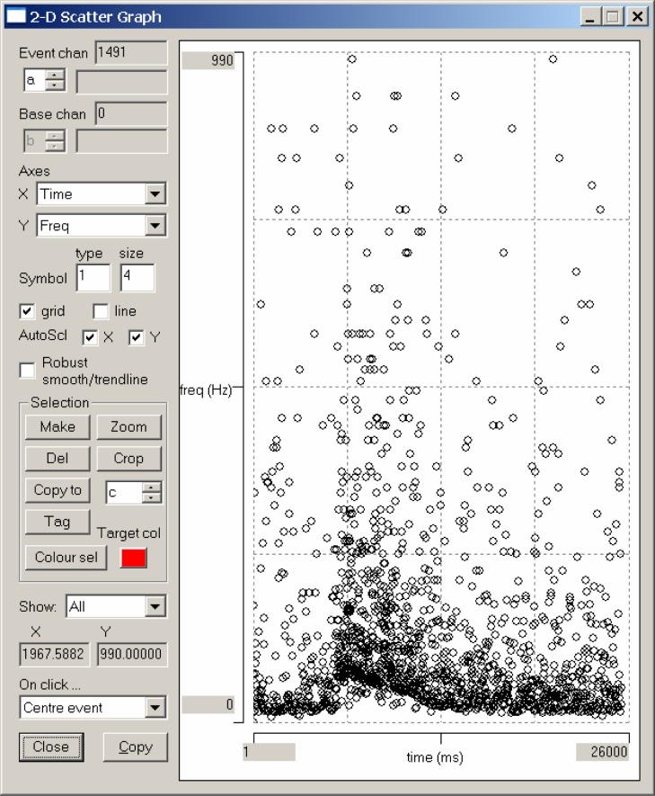
Select the Event analyse: 2-D scatter graph menu command. As its name suggests, this displays a 2-D scattergraph of various parameters. The default display is of time (X-axis) versus instantaneous frequency (Y-axis), which is just what we want. The scattergraph confirms that there is an increase in frequency during the light stimulus, but the display is very “messy” (Fig. 3). Furthermore, the peak frequency is about 990 Hz, which is clearly impossible for a single axon. This strongly suggests that the allowed error for the template match has been set too liberally – a notion confirmed by the fact that all three of the spikes visible in the expanded window have events associated with them, despite the fact that these spikes clearly have different shapes. We need to reduce the allowed error, but can DataView give us a clue as to what an appropriate error might be?

Figure 3.

A scattergraph of time versus instantaneous frequency for events which match the template with an allowed error which has been set deliberately high.

We can observe the numerical values of the error associated with the three spikes in the expanded window by selecting the Event edit: Numerical display: Var val menu option (make sure that the expanded display is active, not the display showing the whole file). “Var val” stands for “variable value,” where the variable in question is context dependent, but in this case is the error relative to the template. The central spike, which was the source of the template, has an error of 0 (which is not surprising), while the other two spikes have errors equal to or greater than 16. This suggests that the error should be set to a value less than 16.

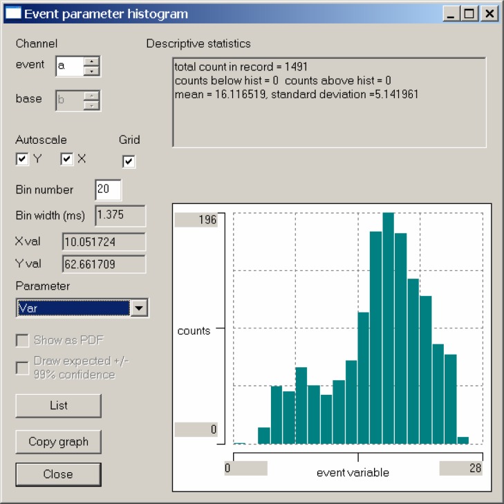
We can get a better clue regarding an appropriate Allowed error value by looking at the distribution of the errors. Select the Event analyse: Histogram/statistics menu command, and a histogram displays. By default this is an interval histogram, but this is not what we want. Select var from the drop-down Parameter list box, and we see a histogram of the error associated with each of the 1491 recognized events (Fig. 4). (Be careful not to press the Enter key at this time, because that will activate the default Close button, which closes the dialog box.)

Figure 4.

A histogram showing the distribution of errors of waveforms that match the template within an allowed error of 25. Note that there is a single event with an error of 0 (the template itself) and that there is a discontinuity in the histogram at an error value of about 10.

There is a clear discontinuity in the histogram at an error value of about 10 (if you hover the mouse over the display you can read the X values from the left of the dialog box), which suggests that this might be a suitable value for the allowed error. Now Close the histogram dialog box.

To see the effect of changing the error clearly, first re-activate the scattergraph dialog box and de-select the AutoScl X and Y check boxes. This will prevent the axes re-scaling automatically as the data change. Now re-activate the Template recognition dialog box and position it so that you can see both the scattergraph and the expanded waveform window, set the Allowed error to 10 and click the Analyse button. Now only 235 spikes are recognized as a match to the template, and in the expanded display, only the template spike itself is recognized as a match. The scattergraph shows spikes with a low, approximately constant, frequency. We can get a clearer view of this by setting the top of the frequency scale to a value of 50. If we look at the upper band of the frequency response (the lower bands will be considered later), we can see that there is a very small and brief change at the time of the light stimulus; but this miniscule response does not seem adequate to explain the display of the actual data, nor the audio playback of the photoresponse. It, therefore, seems unlikely that we have correctly identified the CPR spike.

Changing Templates

We will now use the left-hand spike in the expanded display as a second putative template for the CPR. There are two ways we could do this; we could drag the screen cursors to match the spike, or drag the spike to match the cursors. We will do the latter. Click-and-hold the display screen just above the peak of the left-hand spike, and note that the mouse cursor turns into a blocky left-right icon. Drag the mouse to the right and release it when the mouse cursor is just over the peak of the spike between the two vertical screen cursors. This will shift the display screen to the right and should place the new spike in a suitable position between the screen cursors for capture as a template. The cursor time displays should now read something like 6685.9 and 6686.9 ms.

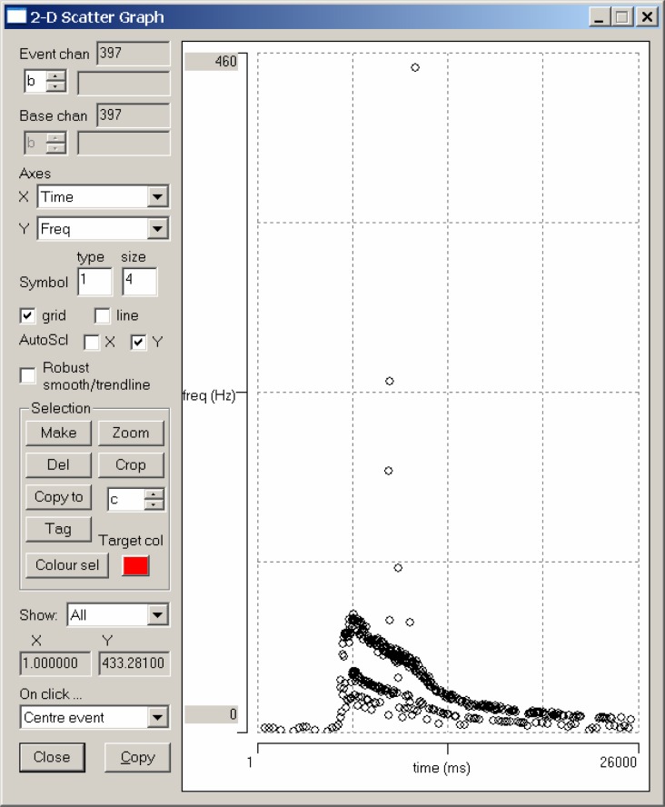
Re-activate the Template recognition dialog box. Click the Capture button, and note how the waveform in the dialog box window changes to reflect the new template. Now change the Event channel (on the right at about the mid-height of the dialog box) to b, so that we do not overwrite the events associated with the previous spike template (in event channel a). Switch to the 2-D scatter graph and check the AutoScl Y box, and select Event chan b (top-left). At this stage the scattergraph will be blank because we do not yet have any events in channel b. Now go back to the Template recognition dialog box and click Analyse. If all has gone according to plan, you should detect about 347 matches to the template, with a very clear photoresponse in the time versus instantaneous frequency scattergraph.

Refining Spike Recognition

The scattergraph shows a clear upper frequency trendline but with four high outliers. These are likely to be false-positive spikes, i.e. spikes that are close to the CPR in shape, but which are not the CPR. There is also a layer of what looks like a different response trendline at one half of the main frequency trend, and perhaps further layers below that. We will look at these in more detail later, but these are probably false negatives, i.e. missed genuine CPR spikes.

One problem with using a single spike picked at random from the record as a source for the template is that all spikes are contaminated by noise; and therefore, even if the spike actually is a CPR spike, it may not be very representative of the “ideal” CPR waveform. However, once we have a template that gives a reasonable result with few false positives, we can improve it by generating a new template from the average of the waveforms that match the original template. Click the Replc w avg (replace with average) button in the Template recognition dialog box and note that the template waveform visible in the dialog box becomes smoother. Now click the Analyse button again. This time 396 spikes are recognized. Two of these are additional false positive high outliers but the remaining newly-recognized spikes fill in gaps in the original frequency trendline (Fig. 5).

Figure 5.

A scattergraph of time versus instantaneous frequency for events which closely match a template derived by averaging the waveforms matching an earlier template which was itself derived from a single spike which probably represented a genuine CPR spike.

We can locate the actual spike pair in the data record which generates a point in the scattergraph by clicking on that point within the graph. The main view will then center in the display the second spike of the pair of spikes generating the frequency (the instantaneous frequency is the reciprocal of the interval between two adjacent spikes). Try this out by clicking on the highest outlier in the scattergraph. The expanded main display (Fig. 6) shows two spikes close together in time, the first of which is a close match to the template, while the second is a poorer match, although it is within the allowed error. Since the instantaneous frequency of this spike pair is almost impossibly high, it is almost certain that one of them is a false positive – and it is likely to be the righthand one with the higher error. (Note that the cursors remain at fixed locations on the screen, but because they are no longer needed, they can be removed with the Cursors: Del all menu command.)

Figure 6.

A spike pair which match the template, but which produce a high frequency outlier. One of the pair must be a false positive.

We can manually remove an event from the record by right-clicking within the inverted U of the event in the main display, and selecting Del one event from the context menu. If you try this while observing the scattergraph, you will see the appropriate high outlier disappear. Obviously, this sort of manual editing involves an element of judgment which obviates one of the advantages of automatic spike recognition – that it is objective, and therefore immune from influence by experimenter expectation. However, in this case the main frequency trend is very clear and the evidence that the outliers are indeed false positives is unambiguous. In less clear-cut cases it is probably better to leave the data un-edited.

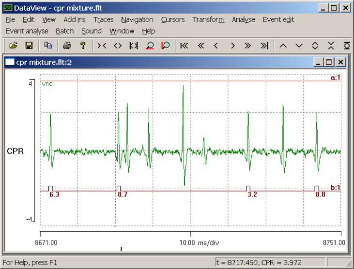
We will now consider the layers below the main trendline visible in the frequency scattergraph, previously claimed as false negatives. We could locate these by clicking on the scattergraph, but there are many to choose from. A good example can be seen by setting the start time of the main display to 8671 ms and the timebase to 10 ms/div (Fig. 7). There are four spikes recognized as the CPR, but where there “ought” to be a CPR spike towards the center of the display, there is instead a large spike which clearly does not resemble the CPR spikes in shape, and so, correctly, has not been recognized as a match to the template. What almost certainly happened here was that the CPR did indeed spike at the appropriate time but so did another neuron. The two spikes added together in the extracellular recording (which represents the voltage generated by the summed extracellular currents of all neurons active at that time) to produce a single “super-spike.” The missed CPR spike means that the interval between the two correctly-recognized spikes on either side is twice as long as usual, and hence the instantaneous frequency drops to half its normal value.

Figure 7.

Spike overlap distorts the waveform of a CPR spike in the center of the display, causing a false negative and a half-frequency outlier. The position of the trace of event channel b has been dragged below the spike waveform for clarity.

Distortion of spike waveforms due to overlap with other spikes is a common problem for all shape-based spike recognition algorithms of extracellular recordings, and it can only be solved by some sort of mixture decomposition (see, e.g. Zhang et al., 2004, or the Spike Sorting Wizard in the DataView tutorial), but that is beyond the scope of this tutorial.

At this stage we have identified and characterized two separate spikes in terms of their frequency response to a light stimulus. The spike marked by events in channel a shows only a very slight change in frequency with the light stimulus, while the spike marked by events in channel b (the CPR) shows a very marked response. We can switch rapidly between the two responses in the scattergraph by using the spin buttons to alternate between Event chan a and b.

Examining Spike Shapes

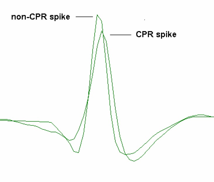
Finally, we may want to look at the shapes of the spikes that we have identified. Select the Event analyse: Draw/average/measure menu command. This shows the superimposed waveform traces at times defined by the events. By default, only 25 waveforms are superimposed; but by setting the Count to −1, we can view all of them (replace the 25 with −1 and press the Tab key – do not press Enter). Switching between Event channel a and b (using the spin buttons located at the top-left of the dialog box) reveals that the two waveforms are clearly different from each other, and that the waveforms are highly consistent within each channel. We can see the averaged waveform of each spike by selecting the Draw: average option (towards the bottom of the dialog box), and these waveforms could then be Copied and Pasted into a drawing program if desired (Fig. 8).

Figure 8.

Superimposed images of the averaged waveforms of two spikes, the strongly photosensitive CPR spike, and a larger very weakly photosensitive non-CPR spike.

DISCUSSION

This article describes how the spike template recognition facilities in DataView can be used to extract information about the response characteristics of a single photosensory interneuron from an extracellular recording containing the combined activity of many interneurons. Experiments of this type have been used by the author for several years as the basis for final-year undergraduate projects, and in all cases so far students have rapidly become familiar with the program interface and facilities, and have used the program with few problems. There is no doubt that the computer-based analysis allows the students to extract more information from their data than they could by attempting a similar analysis by hand. The experimental procedure (especially the dissection) is probably too complicated to be undertaken by a completely naïve student within a single laboratory half-day session, but it should be well within the capability of students who already have some experience of electrophysiology and/or crayfish neuroanatomy (such as those following the experiments described in the Crawdad package; Hoy et al., 2002). Analysis of the type described in this tutorial, can, of course, be undertaken as a homework exercise outside class time, if desired.

The main advantage of DataView over standard commercial research-based programs is that the unlicensed version is free and even the licensed version is very inexpensive. Despite this low or zero cost, DataView provides analysis routines that are sufficiently sophisticated to enable students to gain experience of the methodologies that they encounter in the primary and secondary research literature. Also, hopefully, DataView has a reasonably friendly and intuitive interface suitable of undergraduate use.

The current version of DataView is a display-and-analysis program only, so how can one get data to feed into DataView? DataView can read files in its own internal binary format, and it can also read files in standard text format, and receive data from the clipboard which have been copied there by an external program such as Excel. There are a number of low-cost acquisition systems which can write data in text format (see George, 2006, for a review of several such systems), as can most research-level acquisition programs. DataView can also construct its own files according to mathematical formulae, which can be useful for illustrating the principles of, for instance, digital filtering, spectral analysis, or the Nyquist sampling theory.

A license is available which enables DataView to read several commercial acquisition formats directly, including CED Signal and Spike 2, Axon ABF (currently up to version 9), RC Electronics EGAA, Wintrontech, audio WAV format and plain binary (Labview). A small fee is charged for this license to help defray development and support costs. The author will consider extending support to additional commercial formats on request, so long as details of the format are available. The licensed version could be used by a tutor to translate files from a supported commercial format into the native DataView format, which could then be accessed by students who had installed the free unlicensed version on their own computers.

This article concentrates on one aspect of DataView, but the program contains quite a wide range of data analysis and manipulation facilities. The default installation of DataView includes a comprehensive tutorial manual and sample data set, and perusal of this manual may reveal other facilities of interest to neuroscience educators. The author of the software is a neuroscience educator as well as (occasional) researcher, and is receptive to requests for features which might be of general interest to the neuroscience teaching community (although offers no guarantee that such requests can be fulfilled).

REFERENCES

- George S. Data acquisition and display for electrophysiology: PC oscilloscopes. J Undergrad Neurosci Ed. 2006;5:R11–R14. [PMC free article] [PubMed] [Google Scholar]
- Harris KD. 2000–2002. http://klustakwik.sourceforge.net.
- Hoy RR, Johnson BR, Wyttenbach RA. Crawdad: A CD-ROM lab manual for neurophysiology. Sunderland, MA: Sinauer; 2002. [Google Scholar]
- Lewicki MS. A review of methods of spike sorting: The detection and classification of neural action potentials. Network: Comput Neural Syst. 1998;9:R53–R78. [PubMed] [Google Scholar]
- Prosser CL. Action potentials in the nervous system of the crayfish. II. Responses to illumination of the eye and caudal ganglion. J Cell Comp Physiol. 1934;4:363–377. [Google Scholar]
- Van Harreveld A. A physiological solution for fresh water crustaceans. Proc Soc Exp Biol Med. 1936;34:428–432. [Google Scholar]
- Welsh JH. The caudal photoreceptor and responses of the crayfish to light. J Cell Comp Physiol. 1934;4:379–388. [Google Scholar]
- Wilkens LA, Larimer JL. Photosensitivity in the sixth abdominal ganglion of decapod crustaceans: A comparative study. J Comp Physiol A Neuroethol Sens Neural Behav Physiol. 1976;106:69–75. [Google Scholar]
- Zhang PM, Wu JY, Zhou Y, Liang PJ, Yuan JQ. Spike sorting based on automatic template reconstruction with a partial solution to the overlapping problem. J. Neurosci. Methods. 2004;135:55–65. doi: 10.1016/j.jneumeth.2003.12.001. [DOI] [PubMed] [Google Scholar]