Teaching Neuroinformatics with an Emphasis on Quantitative Locus Analysis

Abstract

Although powerful bioinformatics tools are available for free on the web and are used by neuroscience professionals on a daily basis, neuroscience students are largely ignorant of them. This Neuroinformatics module weaves together several bioinformatics tools to make a comprehensive unit. This unit encompasses quantifying a phenotype through a Quantitative Trait Locus (QTL) analysis, which links phenotype to loci on chromosomes that likely had an impact on the phenotype. Students then are able to sift through a list of genes in the region(s) of the chromosome identified by the QTL analysis and find a candidate gene that has relatively high expression in the brain region of interest. Once such a candidate gene is identified, students can find out more information about the gene, including the cells/layers in which it is expressed, the sequence of the gene, and an article about the gene. All of the resources employed are available at no cost via the internet. Didactic elements of this instructional module include genetics, neuroanatomy, Quantitative Trait Locus analysis, molecular techniques in neuroscience, and statistics—including multiple regression, ANOVA, and a bootstrap technique. This module was presented at the Faculty for Undergraduate Neuroscience (FUN) 2011 Workshop at Pomona College and can be accessed at http://mdcune.psych.ucla.edu/modules/bioinformatics.

Neuroinformatic tools are being widely used by neuroscientists to deduce and induce conclusions about genes, the nervous system, and behavior. As undergraduate students enter into the increasingly interdisciplinary field of neuroscience, they will need to be conversant with a variety of resources that connect the fields of genetics and neuroscience. This module incorporates several neuroinformatic tools in a package enabling students to understand how a candidate gene associated with a particular physical or behavioral phenotype might be identified. In the process, students travel the same experimental road that current neuroscientists use to delve into databases and extract relevant information to both inform and to direct their research.

The entire Neuroinformatics module described here is in silico, and uses resources that are available at no cost on the web. Students begin the project by quantifying a neuroanatomical phenotype using ImageJ, a free, downloadable program produced by the National Institutes of Health (NIH, 1997), in conjunction with digitized brain slice data obtained from the Mouse Brain Library (Rosen et al., 2000). After working in small groups, the class comes together to “clean up” the data using multiple regression procedures that remove the variance due to extraneous variables and creates the statistical data required for a Quantitative Trait Locus (QTL) analysis.

The linchpin of this module is making the intellectual connection between neural phenotype and underlying genetic variation using WebQTL (Zhou, 2011), a free tool that performs QTL analysis, by linking differences in phenotype to loci on chromosomes that likely had an impact on the phenotype (Grisel, 2000). WebQTL conveniently links directly to the UCSC Genome Browser (USCS Genome Bioinformatics Group, 2011), which allows students to move directly to individual loci and begin screening genes using a variety of criteria including microarray expression data provided by the genome browser itself, in situ hybridization analysis with the Allen Brain Atlas (Allen Institute for Brain Science, 2009), coding sequence information in NCBI’s Entrez Gene (NCBI, 2011b), and published literature in PubMed (NCBI, 2011c).

As a whole this module uses several websites in concert to teach genetics, some neuroanatomy and histology, statistics, QTL analysis, molecular biology including in situ hybridization and microarray analysis, and introduces bioinformatic resources. The modular nature of the project allows it to be incorporated into diverse classroom settings, including teaching laboratories and lecture-only courses, providing flexibility to meet specific course and institutional needs.

MATERIALS AND METHODS

Step 1: Selecting the phenotype

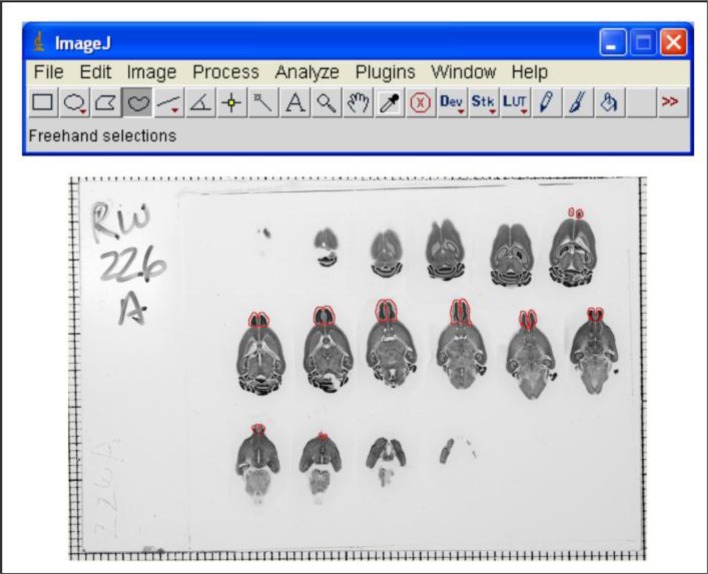
Brain images are obtained from the Mouse Brain Library. These are the extracted and Nissl-stained brains of recombinant inbred mice (See Figure 1). Recombinant inbreeding allows for genetic diversity across strains while keeping genetic diversity within strains fairly uniform. Recombinant inbred strains (RISs) are derived from two inbred F0 strains that are discrepant on the phenotype of interest. By means of recombination of the chromosomes during meiosis in the F1 generation, both genetic and phenotypic diversity across the various strains is obtained. Ultimately, this process derives several inbred strains that are each a unique combination of the F0 DNA but which are homogeneous within a given RIS at all alleles. For a good basic background on simple inheritance, recombination, and inheritance of complex traits see Chapters 5 and 6 of Bazzett, 2008. Details on deriving RISs can be obtained from Grisel, 2000 and Silver, 2008.

Figure 1.

Image from the Mouse Brain Library showing Nissl-stained brains in horizontal sections. Olfactory bulb is outlined in sections in which it appears. Also shown is a toolbar from ImageJ, the program that students use to quantify the size of olfactory bulbs.

The brains in the Mouse Brain Library come from individuals of both sexes and from a wide range of ages, body sizes, and overall brain sizes. The phenotype typically used in this module is olfactory bulb size, because students can easily adhere to an operational definition of what should be measured (see our website materials). For the purposes of this study, the C57BL/6J and DBA/2J strains were used as F0 strains due to their divergent olfactory bulb phenotypes. Also, an article about performing a QTL analysis on olfactory bulb size has been published (Williams et al., 2001), so students can compare their data to published data.

Step 2: Quantifying the phenotype

Students quantify the size of the region of interest using ImageJ. Details on quantifying phenotypes such as olfactory bulbs can be found in the Complete User Manual, on the Neuroinformatics module webpage of the Modular Digital Course in Undergraduate Neuroscience Education (MDCUNE) website at http://mdcune.psych.ucla.edu/modules/bioinformatics. Generally, there is more than one student quantifying the region of interest for a given mouse, which provides a check against other students quantifying the phenotype in a wildly idiosyncratic fashion. Although multiple raters should give better measurements, their data may diverge especially if all raters are not rigidly adhering the operational definition of the phenotype. In cases of divergent measurements, students convene as juries to determine the cause of discrepancies among their measurements and modify them if need be. (Large amounts of error variance will work against getting statistically significant results.)

Step 3: Isolating the genetic contribution to phenotype

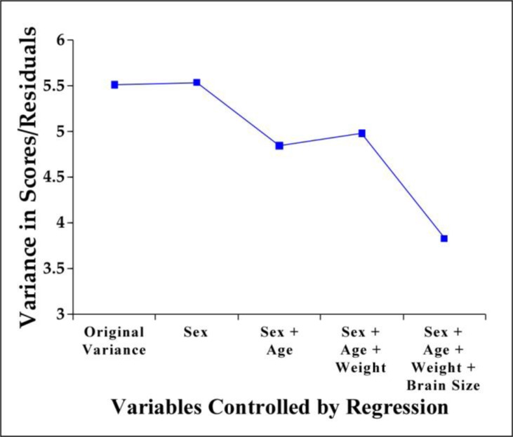
Although the goal of this module is to examine the effects of genes specific to olfactory bulb size, the contributions of these specific genes may be obscured by the influence of other, previously mentioned factors. Consequently, it is imperative to remove the contributions of these other factors (sex, age, weight, and brain size) and control for these factors statistically via multiple regression. Free software, such as Smith’s Statistical Package (Smith, 2011), is available on the web that will do this in a stepwise fashion. When students graph the variance in scores as extraneous variables are successively controlled, they can see that error variance is being removed (see Figure 2).

Figure 2.

Variance in scores as a function of the variables controlled by regression. When students graph the original variance and residuals like this, they can visualize that variance due to extraneous factors is controlled via multiple regression.

Subsequently, once sex, age, weight, and brain size have been statistically controlled, students can see if there are still differences among RISs in the residual scores. This can be accomplished by using a one-way analysis of variance (ANOVA) with strains serving as the various levels. At present, the statistical analysis program, SPSS (IBM, 2012), is used because it is able to handle a large number of levels in an ANOVA. SPSS also returns an R², which is an estimate of variance accounted for by strain and is also an estimate of the heritability of the trait (see Table 1). The subsequent QTL analysis is currently sensitive when at least 10% of the variance is accounted for by genotype, which is strain in this case (Williams, 1998). Some institutions may not have licenses for SPSS or may not have the time to incorporate full statistical analysis in their class. In these cases, the raw statistical analysis can be done by the instructor, and then the results can be explored by the students in class. This approach was successfully used at the College of Charleston.

Table 1.

ANOVA table showing that there are still differences due to strain after the extraneous variables have been removed. Further, the R² shows that the trait is sufficiently heritable for a QTL analysis to work.

Tests of Between-Subjects Effects
Dependent Variable: Unstandardized Residual
Source	Type III Sum of Squares	df	Mean Square	F	Siq.
Corrected Model	331.463a	36	9.207	1.858	.009
Intercept	.027	1	.027	.005	.942
Strain	331.463	36	9.207	1.858	.009
Error	485.600	98	4.955
Total	817.063	135
Corrected Total	817.063	134

^a.R Squared = .406 (Adjusted R Squared = .187)

Step 4: Performing the QTL analysis

The residuals from the multiple regressions can then be used to perform a QTL analysis. This analysis can be easily accomplished by using WebQTL (Rosen et al., 2000). Averages of the residuals within a given RIS are entered, and then WebQTL uses over 3500 markers (mostly micro satellites across the genome that differ between the F₀ mice) to sort the RISs according to the F0 DNA at a given locus. Once sorted, the residual phenotypes of the various strains are then compared via the Likelihood Ratio Statistic (LRS) calculated at each marker. If the phenotypes with the C57BL/6J DNA are markedly different than the RISs that possess the DBA/2J DNA at a given locus, the LRS will be high; if the respective phenotypes are roughly equal, it will be low. This process is performed at each of the markers that distinguish between the two F0 DNAs. WebQTL displays the LRS as a function of these various markers on chromosomes 1–19 and X (see Figure 3). (Notably, the Y chromosome doesn’t recombine, so this analysis cannot be used with genes associated with it.)

Figure 3.

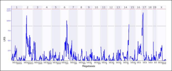
Output from WebQTL of the QTL analysis showing the Likelihood Ratio Statistic as a function of markers across chromosomes 1–19 and X. In this term, students found suggested peaks on chromosomes 2, 6, 14, and 17, which suggests that genes that affected the phenotype are to be found in the regions of chromosomes corresponding to the peaks. [Source: http://www.genenetwork.org/]

In Figure 3, the LRS graph gives four peaks, one each for chromosomes 2, 6, 14, and 17. Although these peaks exceeded the “suggested” criterion (lower horizontal line), none exceeded the “significant” criterion (upper horizontal line). Instructors should not be concerned if their students cannot generate data that exceed the significant level. Because a large number of individual comparisons are made (about 3500),, the alpha level for an individual comparison is extremely stringent, roughly α = 1.5 × 10⁻⁵, to end-up with a compounded, genome-wide comparisons at α = .05. So, it is quite difficult for a given comparison to achieve the significant level even when the null hypothesis is false. Also, suggested peaks are often reported in the literature; QTL analysis is an initial exploration to reveal candidate genes that may impact the phenotype. In addition, if several undergraduates are contributing to the measures, the error variance probably will be large because they will probably not all adhere to the same definition of the phenotype, which will work against obtaining significant results.

Step 5: Linking to UCSC Genome Browser

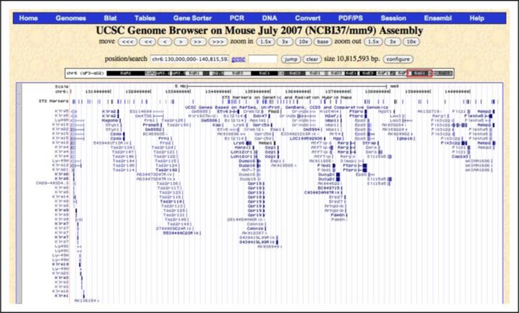
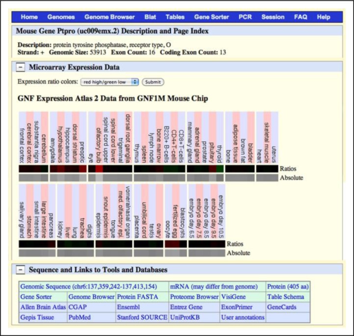
WebQTL links directly to the UCSC Genome Browser, which displays the names of genes under the peak obtained after LRS analysis (Figure 4). These names are linked to information on the relative expression of that gene in several neural regions of interest (Figure 5). Instructors can use these expression data to introduce microarrays and explain how they work. (For an excellent animation explaining microarrays see the DNA Microarray Methodology - Flash Animation from Davidson College, 2001). Students work through the list provided by the UCSC Genome Browser until they find one that is highly expressed in the region of interest. This gene will become their candidate gene.

Figure 4.

Screenshot from the UCSC Genome Browser listing the genes in the distal end of chromosome 6 corresponding to the peak. These genes are hot-linked to information such as expression data of the gene in the region of interest. [Source: http://genome.ucsc.edu/]

Figure 5.

Pastiche of screenshots from the UCSC Genome Browser showing expression data in various regions of interest, the name of a candidate gene, and hot links to obtain more information about this gene including the Allen Brain Atlas, Entrez Gene, and PubMed. [Source: http://genome.ucsc.edu/]

Step 6: Linking to the Allen Brain Atlas (via UCSC Genome Browser)

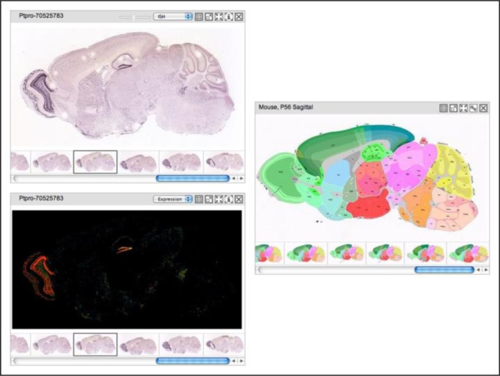
Students then examine the in situ hybridization pattern of their candidate gene using the Allen Brain Atlas. The UCSC Genome Browser links directly to the Allen Brain Atlas, which contains a library of in situ hybridizations done on mouse brains (Ramos et al., 2007). Many genes have been examined in this resource and both coronal and sagittal views of brain sections are available. As seen in Figure 6, the Allen Brain Atlas provides a reference atlas, in situ views, and an expression mask that allows students a more clear view of the brain regions that express their gene. This tool allows students to examine the structures and cell layers within their region of interest that express their candidate gene. Further, it gives students the opportunity to employ a brain atlas and learn some neuroanatomy.

Figure 6.

Pastiche of screenshots from the Allen Brain Atlas showing the in situ view in the top left panel, an expression mask in the bottom left panel showing degree of expression, and a view of the atlas for the corresponding sagittal sections in the right panel. [Source: http://www.brain-map.org/]

Step 7: Linking to Entrez Gene (via UCSC Genome Browser)

The UCSC Genome Browser also has a direct link to Entrez Gene. Here, students are further linked to GenBank (NCBI, 2011a), which provides the full sequence as well as the coding sequence of their candidate gene. Instructors can use this opportunity to explain how one could then construct in situ probes for use in developmental investigations, or for quantitative polymerase chain reactions (PCR). Further, if one knew the coding sequence, it is possible to translate it into a protein and make antibodies to examine the role of this protein in development.

Step 8: Linking to PubMed (via UCSC Genome Browser)

The UCSC Genome Browser also links directly to PubMed, which provides a list of articles about the candidate gene. Students can then find out some information about the gene, including if it potentially played a role in differential development.

Evaluation of Students

At the College of Charleston, a series of short assignments were given that were modeled on the assignments created at UCLA. These short assignments were handed in at the end of each section to ensure that students were staying on task, completing the module, and understand what they were doing. At the end of the module, an individual exam was completed in class to test their understanding of QTL analysis and of the overall module. At UCLA, students were simply given a written take-home exam to assess performance. At both institutions, students who agreed to participate in the study were also assessed by taking a short pre-module evaluation (Pre-Test) and an identical post-module evaluation (Post-Test) that included questions regarding module content, statistical knowledge, and critical thinking. One item on both the Pre-Test and the Post-Test was excluded from analysis because the wording was inadvertently changed between the evaluations taken by College of Charleston students and UCLA students. The assessment measures had IRB approval (UCLA IRB Exemption # 07-211).

RESULTS

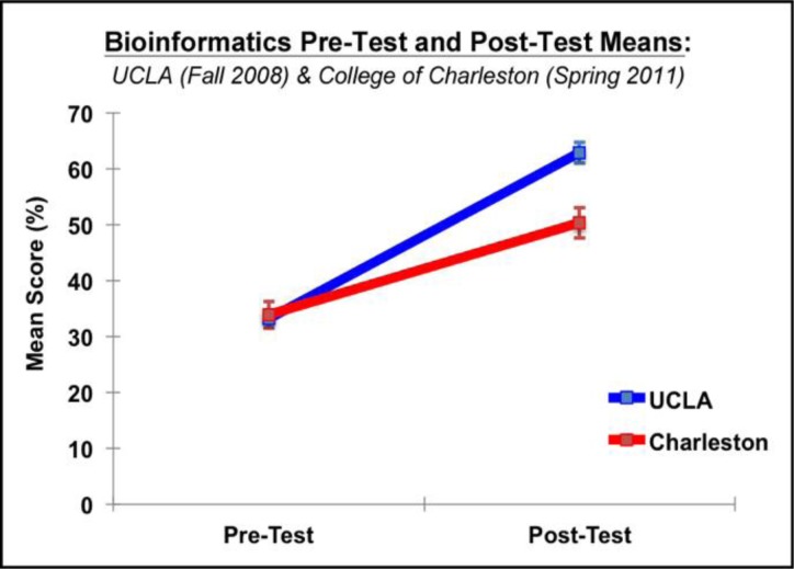
This module has been successfully taught at the College of Charleston and UCLA. Forty-one students from College of Charleston and ninety-two students from UCLA participated in the Pre-Test and subsequent Post-Test that measured gains in content, statistical knowledge, and critical thinking. Students at both institutions made significant strides—Post-Test scores were significantly higher than Pre-Test scores: F(1,131) = 209.91 p < .0001 (Figure 7). The Pre-Test scores did not significantly correlate with the grades on the module at either institution (Table 2), suggesting that module grades at both institutions reflected genuine gains in understanding rather than differential preparation before beginning the course. Grades on the module significantly correlated with the Post-Test scores, providing a measure of validity for the pre-posttest instrument. Although College of Charleston and UCLA students did not significantly differ in Pre-Test scores, there was a significant school x Pre-Test/Post-Test interaction: F(1,131) = 12.18; p = .0008—UCLA students performed better on the Post-Test: t = 3.73; p = .0003 (Figure 7). Both College of Charleston and UCLA students showed reasonable mastery of the material even though different means of assessment were used at the two institutions.

Figure 7.

Mean correct in the Pre-Test and Post-Test for College of Charleston and UCLA students. Significant gains were made by both groups of students as a function of experiencing this module.

Table 2.

Correlation matrix, showing the relationship between module grade and Pre-Test and Post-Test scores, as well as the relationship between Pre-Test score and Post-Test score.

UCLA (n = 92)			College of Charleston (n = 41)
	Pre-Test	Post-Test		Pre-Test	Post-Test
Module Grade	0 180	0.547**	Module Grade	0.090	0.479*
Pre-Test		0.241*	Pre-Test	0.249

^*p < .05;

^**p < .0001

Although we did not measure affective/attitudinal responses to this module in the Charleston students, UCLA students usually made positive comments about this unit (Grisham et al., 2010).

DISCUSSION

The data clearly show that this module worked well at both the College of Charleston and UCLA. At both institutions, students made impressive gains on the Post-Test relative to the Pre-Test. Further, since the module grades were not significantly correlated with the Pre-Test scores but were significantly correlated with the Post-Test scores, the change in scores can be attributed to genuine gains rather than differential preparedness.

UCLA students made larger gains than the College of Charleston students, but at least part of this difference was due to the differential emphasis on statistics. At UCLA, a substantial statistics component was included in this unit: students had to use and understand multiple regression, ANOVA, a permutation test, and the LRS. At the College of Charleston, students did not independently perform the statistical analyses. Rather the instructor completed that aspect of the module and then led a student exploration of the results. Removing the Pre-Test and Post-Test items relating to statistics attenuated this difference between the two schools (data not shown). In other words, the difference in gains exists because UCLA students were taught more “toward the test” than were the College of Charleston students. Although the students at the two institutions were assigned grades by using different measures, students at both institutions showed an adequate mastery of the material—in other words, this module didn’t seem beyond the grasp of students at either institution, and most students successfully completed the module at both institutions.

UCLA students typically find this emphasis on statistics one of the more challenging but valuable lessons from this module. Nonetheless, some students may not have the background for intensive use of statistical analyses or analysis packages may not be available. (Notably, free statistical software can be found online (Pezzullo, 2010), though none of these has been tested for their effectiveness in the Neuroinformatics module.)

This module is centered around QTL analysis of a mouse brain phenotype, but QTL analyses are also being performed on humans to determine the genetic bases of a variety of physical and behavioral phenotypes including ADHD (Doyle et al., 2008), IQ (Butcher et al., 2008), alcoholism (Grisel, 2000;), and dyslexia (Deffenbacher et al., 2004). So QTL analysis has both clinical relevance as well as research utility, and it is an analytical technique with which students should have some understanding.

Similarly, bioinformatics tools such as the UCSC Genome Browser, the Allen Brain Atlas, Entrez Gene, and PubMed, are commonly used by neuroscientists. Students studying neuroinformatics should be exposed to and have familiarity with these tools, since they are re-formulating how neuroscience, biology, and medicine are being approached. The Neuroinformatics module could serve as a stand-alone module or as an adjunct to a genetics or behavioral genetics course.

In the module detailed in this article, the olfactory bulb was used as the phenotype. However, several other brain phenotypes could have been used instead. Potential brain phenotypes about which there are published QTL analyses include cerebellum size (Airey et al., 2002), corpus callosum area (Roy et al., 1998), striatal volume (Rosen et al., 2009), cortex size (Beatty and Laughlin, 2006), amygdala structure (Mozhui et al., 2007), and hippocampus (Peirce et al., 2003; Lu et al., 2001). Anecdotally, there has been better success with olfactory bulbs as a dependent measure relative to cerebellum, cortex, and hippocampus. Students are much more likely to obtain at least suggested peaks when using olfactory bulbs, probably because its anatomical limits are easier to define and quantify.

Logistics

We have endeavored to make this module easy to adapt by instructors at other institutions. All the tools and websites employed in this exercise are free of charge to end-users. In addition, while the project fits well into several lab periods, the individual analyses done at each step can easily be broken down to fit into shorter 50–75 minute class periods within a lecture course. Running the complete module in a typical Monday-Wednesday-Friday 50-minute class schedule at the College of Charleston required a total of about three weeks of class time. At UCLA, three 3-hour lab periods for data acquisition and analysis and three 1-hour lectures were characteristic to provide students with adequate background explanations and guide them in the interpretation of their data.

On the Neuroinformatics module webpage of the MDCUNE website, instructors can find the images of mouse brains that have been used in the unit, and data about each mouse (sex, age, weight, and brain size)—all courtesy of the Mouse Brain Library. The Neuroinformatics module webpage also provides a Complete User Manual, PowerPoint lecture slides with voice-overs, links to videos of live lectures, and individual instructional tutorials on using ImageJ, running statistical analyses, using WebQTL, the UCSC Genome Browser, the Allen Brain Atlas, Entrez Gene, and PubMed. Further, faculty can also access both multiple choice and essay exams along with grading keys after registering for an account with MDCUNE.

Students often comment in formal and informal feedback that they like seeing how elements that they have learned in isolation—genetics, statistics, brain anatomy, and molecular biology—can come together to create a unified story. All of these materials are available to faculty and students to re-create this experience at their home institutions at http://mdcune.psych.ucla.edu/modules/bioinformatics.

REFERENCES

- Airey D, Lu L, Shou S, Williams RW. Genetic sources of individual differences in the cerebellum. Cerebellum. 2002;1:233–240. doi: 10.1080/147342202320883542. [DOI] [PubMed] [Google Scholar]
- Allen Institute for Brain Science Allen Brain Atlas: Home. 2009. http://www.brain-map.org/ (accessed 24 March 2009).
- Bazzett TJ. An introduction to behavior genetics. Sunderland, MA: Sinauer Associates; 2008. [Google Scholar]
- Beatty J, Laughlin RE. Genomic regulation of natural variation in cortical and noncortical brain volume. BMC Neurosci. 2006;7:1–10. doi: 10.1186/1471-2202-7-16. [DOI] [PMC free article] [PubMed] [Google Scholar]
- Butcher LM, Davis OS, Craig IW, Plomin R. Genome-wide quantitative trait locus association scan of general cognitive ability using pooled DNA and 500K single nucleotide polymorphism microarrays. Genes Brain Behav. 2008;7:435–446. doi: 10.1111/j.1601-183X.2007.00368.x. [DOI] [PMC free article] [PubMed] [Google Scholar]
- Davidson College, Department of Biology DNA microarray methodology - flash animation. 2001. http://www.bio.davidson.edu/Courses/genomics/chip/chip.html (accessed 12 January 2012).
- Deffenbacher KE, Kenyon JB, Hoover DM, Olson RK, Pennington BF, DeFries JC, Smith SD. Refinement of the 6p21.3 quantitative trait locus influencing dyslexia: linkage and association analyses. Hum Genet. 2004;115:128–138. doi: 10.1007/s00439-004-1126-6. [DOI] [PubMed] [Google Scholar]
- Doyle AE, Ferreira MA, Sklar PB, Lasky-Su J, Petty C, Fusillo SJ, Seidman LJ, Willcutt EG, Smoller JW, Purcell S, Biederman J, Faraone SV. Multivariate genomewide linkage scan of neurocognitive traits and ADHD symptoms: suggestive linkage to 3q13. Am J Med Genet B Neuropsychiatr Genet. 2008;147B:1399–1411. doi: 10.1002/ajmg.b.30868. [DOI] [PMC free article] [PubMed] [Google Scholar]
- Grisel JE. Quantitative trait locus analysis. Alcohol Res Health. 2000;24:169–174. [PMC free article] [PubMed] [Google Scholar]
- Grisham W, Schottler NA, Valli-Marill J, Beck LM, Beatty J. Teaching bioinformatics and neuroinformatics using free web-based tools. CBE Life Sci Educ. 2010;9:98–107. doi: 10.1187/cbe.09-11-0079. [DOI] [PMC free article] [PubMed] [Google Scholar]
- International Business Machine (IBM) SPSS software for predictive analysis. 2012. http://www-01.ibm.com/software/analytics/spss/ (accessed 10 January 2009).
- Lu L, Airey DC, Williams RW. Complex trait analysis of the hippocampus: mapping and biometric analysis of two novel gene loci with specific effects on hippocampal structure in mice. J Neurosci. 2001;21:3503–3514. doi: 10.1523/JNEUROSCI.21-10-03503.2001. [DOI] [PMC free article] [PubMed] [Google Scholar]
- Mozhui K, Hamre KM, Holmes A, Lu L, Williams RW. Genetic and structural analysis of the basolateral amygdala complex in BXD recombinant inbred mice. Behav Genet. 2007;37:223–243. doi: 10.1007/s10519-006-9122-3. [DOI] [PubMed] [Google Scholar]
- National Center for Biotechnology Information (NCBI) 2011a. GenBank. http://www.ncbi.nlm.nih.gov/genbank/ (accessed 12 January 2012).
- National Center for Biotechnology Information (NCBI) 2011b. Gene. http://www.ncbi.nlm.nih.gov/sites/entrez?db=gene (accessed 12 January 2012).
- National Center for Biotechnology Information (NCBI) 2011c. PubMed. http://www.ncbi.nlm.nih.gov/pubmed/ (accessed 12 January 2012).
- National Institutes of Health (NIH) 1997. ImageJ. http://rsbweb.nih.gov/ij/ (accessed 19 January 2012).
- Peirce JL, Chesler EJ, Williams RW, Lu L. Genetic architecture of the mouse hippocampus: identification of gene loci with selective regional effects. Genes Brain Behav. 2003;2:238–252. doi: 10.1034/j.1601-183x.2003.00030.x. [DOI] [PubMed] [Google Scholar]
- Pezzullo JC. Free Statistical Software. 2010. http://statpages.org/javasta2.html (accessed on 4 February 2012).
- Ramos RL, Smith PT, Brumberg JC. Novel in silico method for teaching cytoarchitecture, cellular diversity, and gene expression in the mammalian brain. J Undergrad Neurosci Ed. 2007;6:A8–A13. [PMC free article] [PubMed] [Google Scholar]
- Roy IL, Perez-Diaz F, Roubertoux P. Quantitative trait loci implicated in corpus callosum midsagittal area in mice. Brain Res. 1998;811:173–176. doi: 10.1016/s0006-8993(98)00975-5. [DOI] [PubMed] [Google Scholar]
- Rosen GD, Pung CJ, Owens CB, Caplow J, Kim H, Mozhui K, Lu L, Williams RW. Genetic modulation of striatal volume by loci on Chrs 6 and 17 in BXD recombinant inbred mice. Genes Brain Behav. 2009;8:296–308. doi: 10.1111/j.1601-183X.2009.00473.x. [DOI] [PMC free article] [PubMed] [Google Scholar]
- Rosen GD, Williams AG, Capra JA, Connolly MT, Cruz B, Lu L, Airey DC, Kulkarni K, Williams RW. 2000. The Mouse Brain Library at www.mbl.org. Int Mouse Genome Conference 14:166. www.mbl.org (accessed 12 January 2012).
- Silver L. 2008. Mouse Genome Informatics (2008) Lee Silver’s Mouse Genetics (Adapted for the Web). http://www.informatics.jax.org/silver/ (accessed 5 April 2009).
- Smith G. Smith’s Statistical Package. 2011. http://economics-files.pomona.edu/StatSite/SSP.html (accessed 19 January 2012).
- USCS Genome Bioinformatics Group UCSC Genome Bioinformatics. 2011. http://genome.ucsc.edu/ (accessed 22 January 2012).
- Williams RW. Neuroscience meets quantitative genetics: using morphometric data to map genes that modulate CNS architecture. 1998. http://www.nervenet.org/papers/shortcourse98.html (accessed 20 January 2012).
- Williams RW, Airey CD, Kulkarni A, Zhou G, Lu L. Genetic dissection of the olfactory bulbs of mice: QTLs on four chromosomes modulate bulb size. Behav Genet. 2001;31:61–77. doi: 10.1023/a:1010209925783. [DOI] [PubMed] [Google Scholar]
- Zhou X, Yan L, Liu N, Sloan Z, Alberts R, Centeno A, Wang J, Lu L, Manly K, Williams RW. 2011. GeneNetwork. http://www.genenetwork.org/ (accessed 12 January 2012).