Circuit Modeling of the Electrical Impedance Part I: Neuromuscular Disease

Abstract

Multifrequency electrical impedance myography (MFEIM) in the 3 to 300 kHz range was applied to 68 subjects representing 19 different neuromuscular diseases, and the impedances analyzed using the 5-element circuit model. Depending on severity, the “cellular” parameters r₂, r₃, 1/c₁ and 1/c₂ were found to be as much as 10 to 20 fold larger than for normal subjects (taking age and girth into account), but in almost every case the extracellular fluid parameter r₁ was at most only marginally affected. Strong correlations are found between r₂ and 1/c₁, but in the case of ALS that breaks down when c₁ (representing the muscle fibre membrane capacitance) falls below half the normal value. Also, c₂ (tentatively associated with intracellular organelle membranes) was found to be the most sensitive to disease progress in ALS, about 3 times more so than the 50 kHz phase, already suggested for use in clinical drug testing. We conclude that following parameters obtained using the combined MFEIM/5-element circuit analysis scheme offers a reliable, non-invasive and objective way of characterizing muscle in neuromuscular disease or during clinical drug testing.

1. Introduction

Single frequency electrical impedance myography (EIM) is a quantitative and noninvasive method for assessing relaxed muscle, which can be used to follow the course of neuromuscular disease and its treatment (Rutkove et al. 2002). The present paper is the first of two which study whether its multi-frequency version (MFEIM) can effectively disclose underlying anatomical or physiological features of disease when the impedances are interpreted in terms of the “5-element circuit model” for the muscle tissue. Together they demonstrate that the effects of disease on the parameters of the model can be very large, and that the sensitivity and reproducibility of the overall scheme are sufficient to recommend it for clinical use. This first paper concentrates on the magnitudes of the parameter changes found in a retrospective study of 19 different diseases. The second is devoted to healthy subjects, in particular the changes occurring in normal aging, to detailed tests of the reproducibility of the results, and to the assignment of relevant error bars. (For brevity these will be referred to as “Part I” and “Part II in what follows. A third paper dealing with the effects of disuse following bone fracture will be published separately.)

The connection of EIM to muscle health lies in the fact that the impedance is a complex number whose real part, the resistance R, responds primarily to extra- and intracellular fluids, and whose imaginary part, the reactance X, is dominated by the presence and properties of cell membranes. Applications so far have focused on a derived quantity called the phase, θ ≡ arctan(X/R), which has been found to decline with increasing disease severity in many illnesses (Chertow et al. 1995, Rutkove 2009), with disuse atrophy (Tarulli et al., 2009), and with normal aging (Aaron et al. 2006). R, X and θ all depend on frequency, and 50 kHz single frequency measurements were adopted in early EIM work such as just mentioned as a matter of convenience, though that severely limited the ability to interpret the results in terms of underlying physiology. The multifrequency version exposes qualitative as well as quantitative differences between impedances of healthy and diseased muscle, particularly as disease progresses (Esper et al. 2006, Shiffman et al. 2008), and the challenge to MFEIM is to see if physiological changes accompanying illness can be quantitatively assessed by analysis of the evolving frequency dependencies.

A standard approach to such questions is to represent the tissue by an electric circuit in which resistors represent current paths through extra- and intra-cellular fluids and capacitors represent membranes between compartments. The “3-element model” has been widely adopted (Barsoukov and MacDonald, 2005, Schwan, 1957), but it has been our experience that it invariably fails to adequately fit the multi-frequency EIM data over a wide frequency range. We have adopted instead the 5-element variant illustrated in figure 1 (Kashuri et al. 2007, Shiffman et al. 2008), which one sees reverts to the 3-element version on omission of c₂ and r₃. Its superiority over the older model is demonstrated by figure 2, which shows R(f) and X(f) data in the 3 to 300 kHz range for the medial gastrocnemius of a healthy 21 year old male, together with the least squares fits to the two models. Simply put, the 3-element model does not fit the data at all well, particularly the reactance which is critical for studying intracellular effects. Furthermore, since the 3-element circuit has come to be associated with the much used Cole and/or Cole-Cole models (cf. e.g. Barsoukov and MacDonald, 2005) it is important to point out that the results shown in fig.(2) also mimic the predictions of those models when they are expressed in terms of X vs R plots. That is, to a precision of about 3 %, the X vs R version of fig. (2) is a semicircular arc with centre below the real axis (by about 2.4 ohms.) However, the Cole and Cole-Cole models intrinsically involve a “Constant Phase Element”, for which there is neither need or justification here; the ideal-component 5-element circuit is capable of accurately representing the impedance data without involving a nonlinear entity which has no known tissue counterpart. (We note also that McAdams and Jossinet (1996) have given a thorough analysis of the pitfall of combining circuit models with the “Cole-Cole” representation.)

Figure 1.

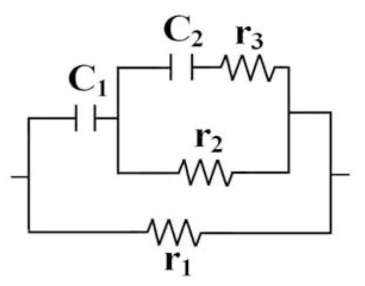
The 5-element circuit used in the MFEIM analysis. (Removing c₂ and r₃ restores the standard 3-element circuit.)

Figure 2.

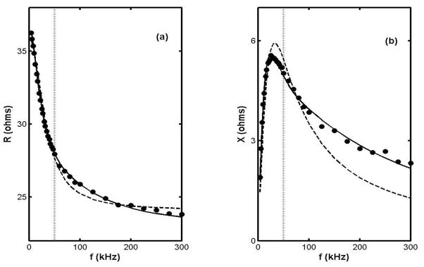
Frequency dependencies of R and X for the right MG of a healthy 21 year old male subject (circles) and the least squares fits to the 5 and 3 element models (solid and dashed curves, resp.) The dotted line is drawn at f = 50 kHz. [The “best fit” parameters are r₁ = 36.6, r₂ = 84.4, r₃ = 224 (ohms), c₁ = 0.0554, and c₂ = 0.00498 (μF), and r₁ = 36, r₂ = 73 (ohms) and c₁ = 0.047 (μF), resp.]

The quality of a fit is no guarantee that the parameters of a model can easily be identified with specific features of the muscle anatomy, of course. Indeed no 5-parameter mathematical expression can ever substitute for something as complicated as real muscle. But there are questions which comparisons of the model with the impedance data may be able to answer. For example, to what extent can changes in its parameters (singly or in combinations) be associated with well-defined compartments of the musculature. Similarly can the model distinguish between alterations of the sizes, shapes and spatial arrangements of the underlying anatomical structures (the intrinsic properties of their tissue remaining the same) and changes in intrinsic properties of the tissue (the structural aspects remaining the same.) An ultimate goal of this research program is to answer such questions, but it starts by simply presenting evidence that the effects of disease on the parameters can be very large compared to experimental uncertainties. In so doing it demonstrates that the technique holds promise as a reliable way of quantifying neuromuscular disease status, offering a new, objective and painless tool for the clinician. But some headway has been made in addressing the more fundamental questions as well. In particular the results show that the usual identification of r₁ with extracellular fluids must be further qualified and that correlations between changes in pairs of parameters may prove to be as useful as changes in the values of the parameters themselves.

The investigations to be described here use data acquired over a period of years before the 5-element approach was developed, and the measurements were conducted in a hospital neuromuscular disease clinic, largely by hospital personnel. In both respects this has the advantage that the tests were essentially “blind” to the objectives of the present research, but as is inevitable in any retroactive analysis of data, they suffer from a lack of detailed statistical design. Consequently only descriptive statistics are presented, and few if any inferences are drawn regarding the statistical significance of its conclusions. To do so would require additional, more focused studies, which we hope would be stimulated by this work.

2. Measuring technique and data analysis

2.1 Sketch of the measuring system

The basic features of the apparatus are sketched in figure 3, and a more detailed description is given by Shiffman et al (2008). That work covered frequencies up to 2 MHz, but in the present version the range was limited to the 3 to 300 kHz frequency range. In addition to the impedance, muscle girth was measured at the locations of the voltage electrodes using a standard tape measure, and ultrasound images of the skin-fat layers were obtained using a Terason 2000 Hand Held Ultrasound System (Terason, Burlington MA, USA) with a 5-MHz probe. Very briefly, the system is based on a Signal Recovery Model 7280 lock-in amplifier (Advanced Measurement Technology Inc., Oak Ridge, TN, USA), which supplies alternating current from its reference oscillator to the current electrodes and receives voltages at the voltage electrodes or across a current measuring resistor. The voltage electrodes are adhesive Al/Ag/AgCl strips, 2.5 cm apart along a line parallel to the limb axis (part no. 019-766400, Viasys Healthcare, Madison, WI, USA, cut to half length), and the current electrodes are disposable ground plate electrodes (Viasys part no. 019-400500), placed far from the voltage array, as indicated. The switching box indicated by the dotted rectangle contains the very low input capacitance probe (Tektronix P6243, Beaverton, OR, USA), connected via computer-driven miniature relays to selected voltage electrodes by short, unshielded wires.

Figure 3.

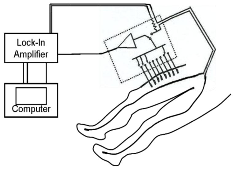
Sketch of the setup for measurements over the quadriceps, showing current electrodes on the feet and a set of voltage measuring electrodes on the thigh. The “z-axis” referred to in the text is an imaginary line along the voltage electrode array, in this case starting 5 cm from the proximalal edge of the patella. (Adapted from Shiffman et al. 2008.)

The figure depicts the voltage electrode array for what is designated as a (right) quadriceps measurement, starting 5 cm from the proximal edge of the patella and extending for 17.5 cm along a line parallel to the axis of the thigh and along its center, as judged visually by the operator. The same practice was followed for the other muscle regions using appropriate anatomical landmarks and voltage electrode arrays 12.5 cm long for the tibialis anterior (TA), medial gastrocnemius (MG) and biceps. The term “forearm” is shorthand for the collection of finger flexors on the anterior forearm, for which the array length was 10 cm. More complete details of these arrays are given in Esper et al. (2006). (Reproducibility of placement relied on the experience of the technician performing the measurements and could no doubt be improved, for example by the use of tattoos. Questions of reliability and reproducibility are considered in detail in Part II.)

2.2. The 5-element circuit

As in the widely used “3-element circuit” the resistor r₁ of fig. 1 is thought to represent the current path through extracellular spaces, c₁ the cell membranes and r₂ the current path through the “intracellular fluid.” The cell interior is extremely complex, and including r₃ and c₂ simply allows for the fact that there are intracellular organelles (Schwan, 1957), with their own membranes and internal fluids. No attempt has been made to assign those parameters to particular features of the cellular anatomy, though the existence of membranes certainly implies the involvement of a new capacitance. (It is interesting to note that the r₂, r₃, c₂ combination is itself a “standard” 3-element circuit.)

2.3. Extraction of the parameters

The parameters are found using a dedicated iterative least-squares program written in Matlab (The Mathworks Inc. Natick MA, USA). In each iteration the program numerically minimizes the combined sum of squares of the deviations of R and X from their theoretical values, but with deviations in X weighted by a factor of 10. Unlike polynomial least-squares procedures, there is no analytic solution to the problem of minimizing the sum of squares, hence the need for an iterative procedure. The search must be given an initial set of parameters, and different choices of starting points can lead to different solutions, often incompatible with gross anatomical aspects of the problem. Additional constraints have been applied to ward against this: the parameters must be positive, must be monotone functions of the length of the voltage measuring interval, z, and must extrapolate to zero at z = 0. In particular r₁, r₂, r₃, 1/c₁ and 1/c₂ should increase with z, the inversion of the last two variables reflecting the fact that capacitive reactance is inversely proportional to the capacitance. Finally, the values assigned to the parameters are governed by the actual value of the current measuring resistor in the dotted enclosure in fig. 3, an ordinary 11 ohm, 5% tolerance carbon resistor. These and other details of the procedure are discussed more fully in “Part II”, the second paper of this sequence.

2.4 Correction for muscle cross-sectional area: “Girth Normalization”

The circuit model makes no provision for different muscular sizes and shapes, and the parameters obtained from it must be adjusted accordingly. A guide to a correction scheme is provided by the expression for the d.c. resistance of a cylindrical conductor, i.e. R = ρ L/A, in which L is the length of the cylinder, A its cross-sectional area, and the resistivity ρ represents the intrinsic electrical properties of the material. To expose those properties one should use values of the resistivity, ρ = R·A/L, rather than values of R alone, and by the same token, in comparing values of the circuit parameters for different subjects one would first have to multiply by the corresponding value of A/L. The muscles are hardly cylindrical, and the best one can reasonably do is to replace A by the area of a circle whose circumference is the average muscle girth over the region spanned by the voltage electrodes (Willan et al., 2002). We measure the surface girth, g, and the thickness of the skin fat layer, sf (using ultrasound), from which we derive an “effective muscle radius” g/2π − sf, and in this approximation the multiplier for the parameters is π(g/2π − sf)²/L. (For this simple geometrical argument to hold it is the values of 1/c₁ and 1/c₂ which must be multiplied by this factor, and in what follows terms such as “capacitive parameters” refers to these inverses, unless indicated otherwise.) Adjustments should be made to take the cross-sectional areas of the bones into account, but for the most part these are small and furthermore difficult to calculate accurately, ranging from 3 to 4% for the femur to 10% for the forearm flexors, according to standard atlas illustrations. There being no way to measure the actual values for our subjects (and only approximate ways to calculate their effect), we have ignored the bone corrections in this analysis. A more serious omission is the possible effect of infiltration of the muscle by fat or connective tissue. This is known to have an effect on muscle strength in the elderly (Lexell et al. 1983, Vandervoort and McComas 1986, Delmonico et al. 2009), and possible effects on the parameters are discussed in section 5.4.

As an example of the effect of girth-normalization, we address what would otherwise appear to be a major discrepancy between r₁ values on the quadriceps and biceps of a 63 year-old healthy female subject. For a L = 17.5 cm length of the quads the average girth was g = 48.4 cm, the skin-fat layer thickness sf = 1.39 cm, and the girth-normalization factor π(g/2π −sf²)/L was 7.87 The uncorrected r₁ value was 26.7 ohms and applying the correction turned this into an “effective resistivity” of 210 ohm-cm. For measurements on the biceps the corresponding figures were L = 12.5, g = 26.3 and sf = 0.28, from which the factor was 3.71. The uncorrected r₁ value was 54.2 ohms, almost twice as large as for the quads, but the corrected value was 201 ohm-cm, only about 4% smaller than that for the quads. (In part II it will be shown that the average zero frequency effective resistivity is 200 ± 19 ohm-cm for all muscles in the full normal group,)

In what follows, the results will be presented as the ratios of the several parameters either to corresponding values measured earlier on the same subject or to the average of values for healthy subjects of the same age group. The first is of course limited to those subjects who were measured more than once, and there the girth normalization procedure is usually of no practical consequence since changes in external girth and skin-fat thicknesses were found to be very small, even over many month intervals. But in the majority of cases assessing the effects of disease required the second approach, and there girth normalization plays a critical role, not only in adjusting for muscle mass of the individual patient concerned but also in forming mass-compensated average parameter values for normal subjects from which the “diseased-to-healthy” ratios are calculated.

In either case, critical attention must be paid to the assessment of measuring errors expected under the conditions prevailing in the clinic. A full discussion of these points would be very cumbersome here, and it has been deferred to Part II. That work focuses on reproducibility of the measuring and analysis system and the sources and magnitudes of system errors, as well as on the properties of the normal “control” group.

3. Subjects

All measurements were conducted at the Department of Neurology of the Beth Israel Deaconess Medical Center. Sixty-eight neuromuscular disease patients representing 19 diagnoses were examined, as delineated in section 4. In a few cases closely related diseases were grouped together, e.g. polymyositis with dermatomyositis, and there were a few infrequent diagnoses for whom extreme impedance behaviour was found, and these are given special attention. There were also 10 subjects with unique diagnoses, and in the interest of brevity these are treated collectively. In addition to the patients with neuromuscular disease, sixty-two subjects showing no evidence of disease were also studied, whose parameters are needed for the calculation of “diseased-to-healthy” ratios just mentioned. (Details of those measurements are given in Part II.) Signed, informed consent was obtained from all subjects and all measurements were conducted in accordance with Institutional Review Board regulations of the Center.

4. Results for various disease groups

4.1. Amyotrophic lateral sclerosis

Twenty-one ALS patients were examined, 12 men and 9 women ranging in age from 30 to 79 years. The time course for development and progression of ALS is several years, and as a practical matter it is almost impossible to demonstrate the full range of impedance variations due to the disease using the data for a single patient. But Table 1 gives three examples illustrating the orders of magnitude that can be expected. In the first, the right quadriceps of one subject had been followed for 4.6 years, though the frequency dependence was measured only at the last visit. At the time of the first, however, the 50 kHz phase (“θ₅₀”) strongly indicated that the disease had not yet affected that muscle, and for present purposes we substitute (girth-normalized) values for a normal subject of the same age and gender. The results are shown in the first segment of the table in the form of final to initial parameter ratios. One also expects parallel contrasts in cases of highly asymmetric diseases, and the second segment of the table shows this for the right-to-left ratios for a subject for whom the clinical assessment at the time of measurement was that the right leg was severely affected and the left leg much less so The third segment of the table shows similar contrasts for widely separated muscles on the same side of a 44 year old male subject, the right biceps and right quads. The first row of the segment shows that there had been little if any change in the right quads over a 188-day period, while the second row shows definite evidence of progressive disease in the right biceps.

Table 1.

“Diseased to healthy” parameter ratios for selected ALS patients

	Muscle	r1	r2	r3	1/c1	1/c2
“t = 0” to 1667 day ratios (see text)	right quads	0.7	3.9	2.5	3.4	3.0
Asymmetric disease right to left ratios	quads	1.1	3.3	2.0	3.9	2.7
	TA’s	0.7	1.7	1.1	2.4	1.5
	MG’s	0.6	1.6	1.1	2.3	1.4
188 day ratios on the same side	r-quads	0.92	0.98	0.94	0.99	0.92
	r-biceps	0.93	1.6	0.87	1.4	1.5

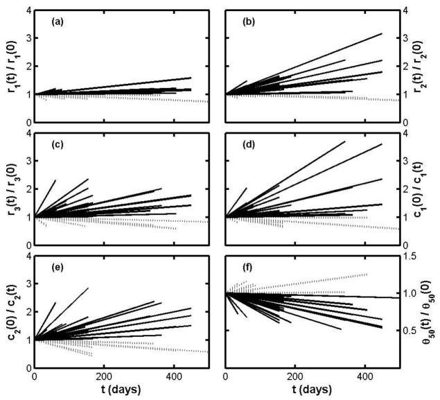
Revisits of many of the ALS patients to the clinic allowed us to make 45 test-retest comparisons, including measurements on relatively spared as well as more severely affected muscles. The results are summarized in Figure 4, in which each line indicates disease progress for a single muscle of a single subject; the ordinate for the end point of a line is the retest-test ratio for the specified parameter, measured over the time interval given by the abscissa. (Note that “t = 0” does not signify the onset of disease but the date of the first measurement of the pair.) Three features stand out: first that some parameters increase three-fold or more in the course of only a year; second that there appear to be periods of relative improvement in some patients (for whom the slopes of the parameter ratios are negative and the 50 kHz phase ratio slopes are positive); and third, r₁ is on the whole very insensitive to disease.

Figure 4.

Figure 4(a–e). Test-retest results for ALS patients plotted as parameter ratios over time, without distinction between clinically affected and relatively spared muscles. Subplot (f) shows the time dependence of the 50 kHz phase. In all the subplots solid lines indicate increasing severity and dashed lines indicate stable or decreasing severity.

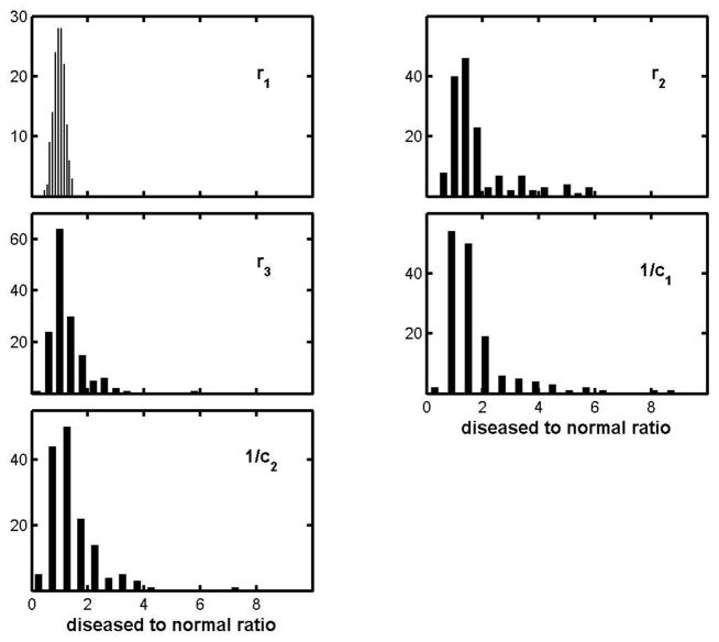
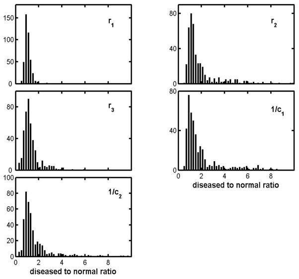
Figure 4 represents only those patients who were examined two or more times, a subset of the whole ALS pool, but one can include subjects for whom there was only one visit by comparing parameter values with those for age-matched normal subjects. Figure 5 does this via histograms of ALS-to-normal parameter ratios. Since there is no objective and quantitative way to characterize disease severity, each histogram includes results for all muscles in each of the 5 of the muscle groups whether there was clinical evidence of disease or not. As a result, each is likely to show a strong peak near ratio = 1, and that is clearly the case. The r₁-ratio distribution is exceptionally sharp and (as will be shown later) it is a good approximation to a Gaussian centered on unity and with a spread compatible with that for healthy subjects (to be presented in Part II.) But while r₁ appears to be largely unaffected by the disease, the effects on the other parameters can be very large, indeed many times larger than can be attributed to measurement uncertainties. For example the largest 1/c₁-ratio is 8.6, and the difference between that and 1.0 (the disease-free value) is about 50 times the uncertainty found for the 1/c₁ ratios for normal subjects. The lack of symmetry makes it difficult to more compactly characterize the histograms, but a fair summary is provided by the mean values, standard deviations and skewness, and these are given for each parameter in the first row table 2. (The table includes corresponding entries for the other diseases, to be discussed shortly.)

Figure 5.

Histogram of diseased to normal parameter ratios for the ALS group.

Table 2.

Group averaged diseased-to-normal parameter ratios: mean ± SD and (skewness).

Disease group	r1	r2	r3	1/c1	1/c2
ALS (21,148)*	1.0±0.2 (−0.01)	1.8±1.2 (1.9)	1.3±0.7 (2.9)	1.8±1.3 (2.7)	1.4±0.9 (2.7)
Radiculopathy(10, 62)	1.0±0.2 (1.6)	1.2±0.5 (1.7)	1.1±0.3 (0.8)	1.2±0.5 (1.5)	1.2±0.5 (2.6)
Poly/dermatoa (13,37)	1.0±0.3 (0.5)	1.6±1.1 (2.3)	1.2±0.7 (2.4)	1.8±1.5 (1.7)	1.5±1.2 (2.7)
CMTb (4,30)	1.3±0.4 (2)	4.9±4.8 (2)	1.9±0.9 (0.6)	4.9±4.1 (1.7)	2.9±2.2 (1.2)
IBMc (4,39)	0.96±0.2 (0.89)	1.9±1.2 (2.3)	1.1±0.6 (0.7)	2.4±1.7 (1.6)	1.6±1.1 (2.2)
Myotonic Dystrd (3,10)	0.94±0.2 (0.55)	3.4±1.8 (0.7)	2.0±0.84 (0.6)	3.8±2.2 (0.5)	2.8±1.7 (0.3)
FSHDe (3,17)	1.3±0.3 (0.07)	2.0±1.1 (1.1)	1.5±0.86 (1.9)	1.8±1.0 (1.0)	1.8±1.1 (1.9)
Othermyopathyf (5,15)	0.99±0.2 (0.9)	2.6±2.3 (1.2)	1.6±1.2 (1.6)	2.1±1.9 (1.5)	2.3±2.6 (1.7)
“ neuropathyf (5,31)	1.1±0.3 (.01)	1.9±2.3 (2.6)	1.4±0.9 (1.4)	1.6±1.5 (2.7)	1.9±2.1 (2.6)
p-values (and sides) g	0.2 (2 sided)	0.0035 (1)	0.0016 (1)	0.0043 (1)	0.0008 (1)

^*(the number of patients, and the number of muscles examined, including lefts, rights, and repeat measurements)

^aPolymyositis and dermatomyositis combined

^bCharcot-Marie-Tooth disease

^cInclusion body myositis

^dMyotonic Dystrophy

^eFacioscapulohumeral muscular dystrophy

^fsee section 4.7

^gNominal t-test values for null hypothesis ratio = 1; cf section 5.1

4.2. Radiculopathies

Ten radiculopathy patients were studied, 8 men and 2 women ranging in age from 46 to 83 years. Ratios of girth-normalized parameters to those for normal subjects of the same age group were calculated as just described, leading to histograms of the same general character; the means, standard deviations and skewness are shown in row 2 of table 2. Judging by the mean values alone, one would conclude that the group was only marginally distinguishable from the normal “controls” of part II, and in fact in about half of the cases there was no significant difference between right and left limb parameters. But as the substantially positive skewness values testify, the range of variation was considerably wider than the standard deviations alone might suggest, the diseased to normal parameter ratios ranging from 0.4 to 2.4.

4.3. Polymyositis and dermatomyositis

Thirteen subjects in our sample had been diagnosed with polymyositis or dermatomyositis, ranging in age from 46 to 80 and including 4 males and 9 females. The impedance findings for the two diseases are very much the same, and the combined group-averaged diseased-to-normal parameter ratios are given in the third row of table 2. Once again the group average ratio for r₁ is very close to one and the standard deviation is modest, but the positive skewness points to a fair degree of asymmetry. Ratios for the “cellular” parameters r₂, r₃, 1/c₁ and 1/c₂ reach levels as high as those found for ALS.

4.4. Charcot-Marie-Tooth (CMT) disease

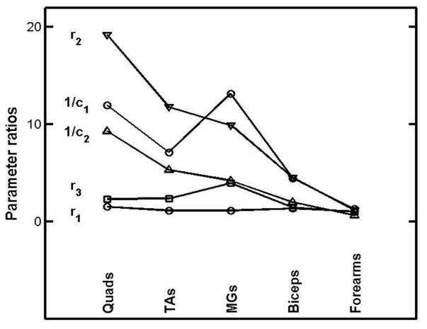
Only four CMT patients were examined, and the average parameter ratios are given in the 4th row of table 2. Standard deviation and skewness have only formal meaning for such a small group (and others to follow), but the very large values found for r₂ and 1/c₁ merit special report. These are shown in Figure 6, in which the “abscissa” is simply a set of integers assigned to the muscles in order to disentangle the lines joining points for the same parameter. Two unexpected features stand out very clearly; the quads show most egregious parameter behaviour, since the disease dominantly affects the lower leg, and there is no sign of disease at all in the forearm parameters.

Figure 6.

Girth-normalized diseased to normal parameter ratios for the left side muscles of a 70 y.o. male suffering from Charcot-Marie-Tooth disease. The abscissae have been chosen simply to disentangle lines joining points for the same parameter.

4.5. Inclusion body myositis (IBM)

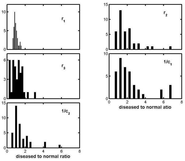
Four patients with IBM were examined. The group averaged ratios are given in the 5^th row of table 2, in most respects exhibiting the same picture as has emerged for the other diseases. But the r₃ ratio is unusual, in that its distribution is heavily weighted towards very small values, as shown by the r₃ histogram in Figure 7. The unusual character of this distribution is particularly interesting, in that the “inclusions” of inclusion body myositis are known to take the form of nanometer-scale cytoplasmic debris, deep within the myocyte.

Figure 7.

Histograms for the parameter ratios of the inclusion body myositis group.

4.6. Myotonic dystrophy and facioscapulohumeral muscular dystrophy (FSHD)

There are only 3 patients in each of these categories, and the parameter ratios fall into the emerging common pattern (lines 6 and 7 of table 2). In particular r₁ is much less influenced by disease, and the other parameters have mean values well above unity, large standard deviations and positive skewness. As before this last indicates very large individual ratios, indeed the 1/c₁ ratio was approximately 8 for the MG of one myotonic dystrophy patient.

4.7. Other Diseases

There were ten patients with diagnoses outside the categories just presented: the myopathies autosomal distal myopathy, mitochondrial myopathy, and Becker’s muscular dystrophy, and the neuropathies axonal polyneuropathy, lumbrosacral plexopathy, peroneal neuropathy, and post-poliomyelitis syndrome. The group averaged parameter ratios are given in the 7th and 8th rows of table 2. Again, large standard deviations and positive skewness indicate large ratios. For example an axonal neuropathy patient with severe weakness in the lower legs had parameter ratios for the right TA reaching almost to 10, i.e. 0.7, 9.7, 2.6, 7.4, and 9.8, in the order r₁, r₂, r₃, 1/c₁, and 1/c₂.

4.8 Correlations between parameters

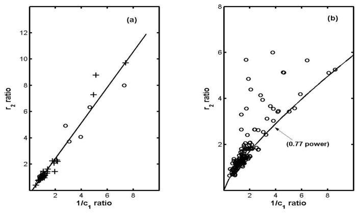
Surveying the various pairs of parameter ratios amongst the diseases exposes a wide spread of correlation coefficients, ranging from a low of 0.26 for the “r₃-1/c₁ coefficient” for IBM (as expected from fig. 8) to a high of 0.99 for the “r₂-1/c₁ coefficient” for the other-neuropathy category. (To avoid very cumbersome notation we use expressions like “the r₃-1/c₁ coefficient” to mean the correlation coefficient between the r₃ diseased to normal ratio and the 1/c₁ diseased to normal ratio.) In fact the r₂-1/c₁ coefficients are relatively high for all the disease groups (mean = 0.91) and furthermore plots of the r₂ ratio vs the 1/c₁ ratio indicate quite good linear dependences. Figure 8(a) shows this for the combined other-myopathies-other-neuropathies group (chosen because its 1/c₁ range is the largest), and Table 3 gives the slopes of linear least-squares fits to such plots for the various disease groups, arranged in order of increasing slope (except in the case of ALS.) Figure (8b) represents the ALS group, for whom the least-squares-fit is limited to r₂ ratios less than 2 for obvious reasons. We return to interpretation of this in section 5.5.

Figure 8.

Correlation and breakdown of correlation between the r₂ and 1/c₁ ratios: (a) open circles for the “other myopathic” and crosses for the “other neuropathic” group, and (b) the ALS group. (The “0.77 power” curve is for emphasis only.)

Table 3.

Slopes of r₂ vs 1/c₁ ratios least squares fitted lines

Disease Group	Slopes ± SD
IBMa	0.62 ±0.06
Poly/dermatomyositisb	0.69 ± 0.04
Radiculopathy	0.73 ± 0.06
Myotonic dystrophy	0.80 ± 0.09
FSHDc	1.06 ± 0.10
CMTd	1.08 ± 0.09
Other myopathiese	1.17 ± 0.08
Other neuropathiese	1.49 ± 0.05
ALS(only for r2 < 2)	0.70 ± 0.07

^aInclusion Body myositis

^bPolymyositis and dermatomyositis combined

^cFascioscapulohumeral muscular dystrophy

^dCharcot-Marie-Tooth disease

^esee section 4.7

5. Discussion

5.1 The stability of r₁ as opposed to the “cellular parameters”

A prominent result of this survey is that the “cellular parameters” r₂, r₃, 1/c₁ and 1/c₂ almost invariably increase with increasing disease severity, reaching levels more than an order of magnitude larger than their normal counterparts, while in contrast the “extracellular fluid” parameter r₁ is largely unaffected by disease. Both features are suggested by the mean values and standard deviations in table 2, but the overall picture is more fairly represented by Figure 9, the combined parameter-ratio histogram for all the diseases. (A few cases with ratios between 15 and 20 have been omitted to avoid overly compressing the remainder of the plots). One can hardly regard these distributions as Gaussian, but nevertheless formal application of conventional t-tests well illustrate the contrast, as shown by the last row of Table 2. Here the null hypothesis is that the diseased-to-normal parameter ratio is equal to 1, i.e. that disease has negligible effect on the individual parameters. As seen, only for r₁ is that tenable (p = 0.2, 2-sided) while for the cellular parameters the individual p-values (1-sided) are extremely small, well below the usually adopted α= 0.05 criterion. (p is even smaller for the set of cellular parameters taken together, i.e. 6 × 10⁻⁸)

Figure 9.

Combined histograms of girth normalized parameter ratios for all the tested diseases and muscles (cut off at ratio = 10).

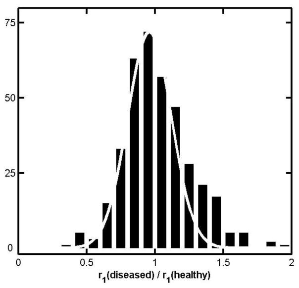
The use of the same abscissa range in all the subplots of Figure 9 emphasizes the narrowness of the r₁ ratio distribution compared to the others, but the common 0.2 bin-width obscures an important additional feature of that distribution. This is remedied by Figure 10, where the bin-width has been cut in half and a Gaussian distribution with standard deviation 0.16 has been superimposed. That value was chosen simply by manual trial and error fitting to the major maximum of the histogram, but it is sufficient to show that there is a strong suggestion of a secondary maximum as well (to which we return below.) That the major part of the distribution is so well centered on unity is evidence that r₁ does not change appreciably under almost all of the tested diseases, regardless of severity. Equally important, the parameter ratios involved here are between individual subjects and average (girth normalized) values for normal controls of the same age group, which themselves have an overall standard deviation of 15.5 % for r₁ according to Part II (males 14%, females 17%). Furthermore, the measurement uncertainty obtained from same-subject test-retest determinations of r₁ is approximately 8.5% (fractional SD), so one expects a combined standard deviation of √ (.155² + .085²) or about 18% for the distribution. That this is so close to the value for the superimposed Gaussian is undoubtedly accidental, but nevertheless the agreement strongly argues that the major part of the observed spread in fig. 10 is much more likely due to intra-group variations and random experimental errors amongst the healthy “controls” than to variations in the properties of the diseased subjects. Furthermore, fig. 10 is evidence of the overall consistency of the parameter extraction scheme, and accordingly the failure of the Gaussian near ratio 1.4 should be taken as evidence that the secondary maximum is not simply a statistical aberration, i.e. that r₁ does change in a minority of diseased subjects. By the same token values well below unity which are found for other parameters in some diseases should also be regarded as true reflections of underlying muscle condition. Of these the most important is the r₃ ratio for the inclusion body myopathies (Figure 7.) Ratios much less than 1 are also found amongst the cellular parameters for the radiculopathy, polymyositis and dermatomyositis patients, albeit only as small fractions of the total numbers in each category. These ratios should now also be regarded as meaningfully low.

Figure 10.

Distribution of r₁ ratios for all diseased subjects combined, together with a Gaussian distribution of standard deviation 0.16

5.2 Pauses in ALS progression

The results for the ALS patients are particularly interesting. By far most of the parameter lines in Figure 4(a – e) have positive slopes, indicating increasing disease severity over time, but there are several showing negligible changes, as well as a few with negative slopes. Correspondingly, positive slopes are found for some of the θ₅₀, as indicated in the sixth subplot of that figure, and we note that initially rising 50 kHz phases have also been reported for some ALS patients by Rutkove et al. (2007). Since a prevailing view is that remissions never occur in ALS, one must ask whether the data are simply in error. Indeed many of the negative parameter slopes in Figure 4 are within one standard deviation of zero (cf. Part II), and only those negative by 2 to 3 standard deviations should be considered. Of these it is very interesting that 15 of those 16 negative slopes are due to only 3 subjects, in fact seven for one alone, and furthermore in one subject negative parameter slopes were found for two successive time intervals. Both of these observations lend support to the hypothesis that the negative parameter slopes are genuine albeit likely to be found in only a small minority of cases. In this connection we note that qualitatively similar reversals of the time course of ALS have been reported for motor unit numbers by Dantes and McComas (1990), also in a minority of cases. A possible explanation is that as motor neurons are lost due to disease there is ongoing reinnervation of muscle by still healthy neighboring motor neurons (Bromberg, 2002). This would help partially restore muscle integrity (at least for a time) and might account for negative parameter slopes, depending on the overall balance of effects throughout the muscle.

5.3 Application to ALS clinical drug trials

θ₅₀ has already been proposed as an outcome measure in Phase II clinical trials for ALS, where many candidate drugs must be screened before undertaking the considerably more challenging Phase III trial (Rutkove et al., 2007). Here we address whether the multifrequency version can offer further advantages, in particular whether any one or a combination of the 5-element circuit parameters is likely to be more sensitive and/or accurate than θ₅₀.

In one way or another the basic strategy of any drug study amounts to monitoring the slope of the q(t) curve, where “q” stands for a variable which reliably assesses the status of the disease. If “m” stands for the slope of q(t) and “δ” specifies the uncertainty in its measurement, then the basic figure of merit for that choice of parameter is Δt ≡δ/m. The larger the slope the less will be the time which is needed, so the immediate question is which parameter would give the largest “m”. Since the parameters have different dimensions, in making comparisons one must use d(log q)/dt for m (which has the added virtue of largely eliminating muscle mass effects), and in our case the logarithmic derivatives are essentially the slopes of the lines in Figure 4. There is a wide range, but for present purposes it is enough to simply take average values and these are given in Table 4. (This includes the θ₅₀ ratio as a sixth entry.) The table shows that choosing any MFEIM parameter except r₁ as the outcome variable offers a roughly two to three-fold time advantage over the 50 kHz phase. Of course, realizing any advantage would depend on the “noise levels” which are encountered, i.e. the “δ” in Δt =δ/m, and formal power calculations would have to be done to properly assess the relative advantages.

Table 4.

ALS group averaged sensitivities: 10³ d(log q)/dt.

q	r1	r2	r3	1/c1	1/c2	θ50
103 d(log q)/dt (days−1)	0.08	1.0	0.98	1.07	1.65	−0.55

5.4 Correlations between parameter changes

As shown in Table 3 and fig. 8a, the r₂ ratios are to a good approximation proportional to the 1/c₁ ratios, but in the case of ALS (fig. 8b) that is true only if the disease is not too far advanced. A form of constrained randomness sets in for 1/c₁ ratio larger than about two, beyond which some mechanism intervenes which manages to leave the entire lower right quadrant of the graph virtually empty. The solid curve in the figure, (r₂-ratio) = (1/c₁-ratio)^0.77, has no fundamental significance and is given simply to draw attention to that feature. But arbitrary as its algebraic form may be, the curve must reflect limits imposed by some natural constraint whose breakdown allows “random” increases in the intracellular fluid parameter r₂ but no decreases. Since the analysis purports to describe the macroscopic muscle by a single circuit, one must consider that dramatic changes in the parameter r₂ could be due either to changes in the internal structure of the affected fibres, with no discontinuous change in their number or spatial arrangement, or to the reverse, a change in the distribution or orientation of the fibres, with no major changes in the fibre interiors. As an example of the first possibility, a disruption of the ordered internal structure of the fibers would increase r₂, leaving c₁ virtually unchanged. On the other hand, since the intracellular current ultimately derives from the extracellular compartment, one cannot rule out that clumping or some other re-distribution of fibres could also have the effect of increasing r₂. As an example, intrusions of fat and connective tissue might be an important factor, as in the case of normal aging (cf. part II).

Lacking biopsy or other micro-scale data one cannot decide which category of causes is appropriate, but comparing figures 8a and 8b shows that the breakdown is not simply a consequence of large 1/c₁ values per se. Correspondingly the explanation is likely to be found in the detailed physiological differences between ALS and the other diseases examined here.

5.5 Connection with the active-to-terminal stage transition in ALS

While each point in fig. 8b represents a different subject (or muscle), the solid “0.77 power” curve can also be interpreted as tracing a typical course of the disease in individual cases. That is to say, at onset the r₂ and 1/c₁ ratios are by definition both unity, and as disease progresses a representative point for an individual moves along the curve until a critical level is reached. The fact that for some ALS patients the point still lies on the curve up to very large 1/c₁ would be interpreted in this scenario to mean that that critical level can be very different for different patients, and similarly the seemingly random distribution of r₂ values above the curve would indicate that the consequences of moving off it can be very different from one subject to another.

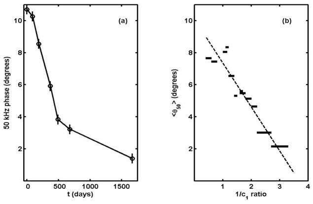
But explanations aside, it should be possible to see evidence of such a scenario by following disease in individual subjects. As noted earlier, there is only one ALS patient whom we have been able to follow for the necessary length of time, (the one depicted in the first segment of table 1) but now at least the 50 kHz phase behaviour can be examined for the whole 4.6 year period. The result is shown in Figure 11(a), which one notes bears a striking resemblance to the dependence of fibre area on time following denervation found by Stonnington and Engel (1973). In any case it is clear that a major change in slope occurred at t ≈ 500 to 600 days, and we have tentatively identified it with the transition from the “active” to the terminal stage of the disease. The phase there was between 3 and 4°, and one can ask if that is connected with the onset of randomness near 1/c₁ = 2 in Figure 8(b). This can be answered by examining the average θ₅₀ for narrow groups of points along the 1/c₁ axis, and the result is shown in Figure 11(b). According to this, θ₅₀ lying between 3 and 4 degrees corresponds to the 1/c₁ ratio lying between 2.2 and 2.6 That is to say, the transition to semi-random behaviour in Figure 8(b) is certainly compatible with the break in slope of Figure 11(a). This in turn suggests that the onset of the terminal stage is characterized by the widespread disruption either of the internal structure of the muscle fibres or of their overall spatial arrangement.

Figure 11.

(a) θ₅₀ vs. time for the quadriceps of the ALS patient of segment 1 of table 1; (b) average θ₅₀ for points of Figure 8(b) lying in the indicated 1/c₁ ratio ranges.

6. Summary

This paper demonstrates that MFEIM and the 5-element model can provide new insights into physiological changes due to disease and, as will be shown in part II, to normal aging as well. Six findings of the research should be investigated under more controlled conditions than were possible in a retrospective study such as this. (1) The “extracellular fluid” resistor of the circuit model, r_1, is largely unaffected by disease, which suggests that it mainly represents the fluids in the vascular system, even though there is twice as much interstitial as vascular fluid in the extracellular compartment. (This will be discussed further in the third member of this sequence of papers.) (2) The general pattern for the “cellular” parameters r₂, r₃, 1/c₁ and 1/c₂ is that with few exceptions all increase with disease severity, independent of disease type, which suggests that features likely to be common to all the diseases are largely responsible, such as atrophy and edema. (3) On the other hand, there is evidence that the slopes of the r₂ vs. 1/c₁ ratio plots may well be different for different diseases. (4) The case of ALS is particularly noteworthy in that the correlation between r₂ and 1/c₁ holds only for relatively early stages of the disease, breaking down completely in later stages. (5) Otherwise, there is only one disease for which one can say there is an identifying “signature” in the pattern of parameter changes, namely inclusion body myositis, for which the changes in r₃ are unique. (6) There are also cases of major changes in parameters which have no parallel with standard clinical descriptions, notably the extreme values found for the quadriceps muscles in a case of Charcot-Marie-Tooth disease, for which involvement of the quadriceps is expected to be minimal.

One result which may find immediate clinical application is the use of the circuit parameters as outcome measures in drug trials for ALS. The intrinsic sensitivities of r₂, r₃, 1/c₁ and 1/c₂ to disease progress are 2 to 3 times higher than that for the 50 kHz phase (currently under study for such purposes), quite likely because the disease-insensitive parameter r₁ no longer contributes.

References

- Aaron R, Esper GJ, Shiffman CA, Bradjonic K, Lee KS, Rutkove SB. Effects of age on muscle as measured by electrical impedance myography. Physiol Meas. 2006;27:953–9. doi: 10.1088/0967-3334/27/10/002. [DOI] [PubMed] [Google Scholar]
- Barsoukov E, MacDonald J. Impedance Spectroscopy, Theory, Experiment and Applications. Hoboken, NJ: Wiley; 2005. [Google Scholar]
- Bromberg MB. In: Neuromuscular function and disease—Basic, Clinical and Electrodiagnostic Aspects. Brown WF, et al., editors. Vol. 1. Philadelphia, PA: WB Saunders; 2002. p. p1311. [Google Scholar]
- Chertow GM, Lowrie EG, Wilmore DW, Gonzalez J, Lew NL, Ling J, Leboff MS, Gottlieb MN, Huang W, Zebrowski B. Nutritional assessment with bioelectrical impedance analysis in maintenance hemodialysis patients. Journal of the American Society of Nephrology. 1995;6:75–81. doi: 10.1681/ASN.V6175. [DOI] [PubMed] [Google Scholar]
- Dantes M, McComas AJ. The extent and time course of motoneuron involvement in amyotrophic lateral sclerosis. Muscle Nerve. 1990;14:416–421. doi: 10.1002/mus.880140506. [DOI] [PubMed] [Google Scholar]
- Delmonico MJ, Harris TB, Visser M, Park SW, Conroy MB, Velasquez-Mieyer P, Boudreau R, Manini TM, Nevitt N, Newman AA, Goodpaster BH. Health, Aging, and Body: Longitudinal study of muscle strength, quality and adipose tissue infiltration. Am J Clin Nutr. 2009;90:1579–1585. doi: 10.3945/ajcn.2009.28047. [DOI] [PMC free article] [PubMed] [Google Scholar]
- Esper GJ, Shiffman CA, Aaron R, Lee KS, Rutkove SB. Assessment of neuromuscular disease with multifrequency electrical impedance myography. Muscle Nerve. 2006;34:595–602. doi: 10.1002/mus.20626. [DOI] [PubMed] [Google Scholar]
- Kashuri H, Aaron R, Shiffman CA. Frequency dependence of forearm muscle impedance during isometric gripping contractions. In: Scharfetter H, Merwa R, editors. IFMBE Proc. 17. 2007. pp. 651–4. [Google Scholar]
- Lexell J, Hendriksen-Larsen K, Winblad B, Sjostrom M. Distribution of different fibre types in human skeletal muscles: influence of aging studied in whole muscle cross sections. Muscle Nerve. 1983;6:588–595. doi: 10.1002/mus.880060809. [DOI] [PubMed] [Google Scholar]
- McAdams ET, Jossinet J. Problems in equivalent circuit modeling of the electrical properties of biological tissues. Bioelctrochem and Bioenergetics. 1996;40:147–152. [Google Scholar]
- Rutkove SB. Electrical impedance myography: background, current state, and future directions. Muscle Nerve. 2009;40:936–946. doi: 10.1002/mus.21362. [DOI] [PMC free article] [PubMed] [Google Scholar]
- Rutkove S, Aaron R, Shiffman C. Localized bioimpedance analysis in the valuation of neuromuscular diseases. Muscle Nerve. 2002;25:390–7. doi: 10.1002/mus.10048. [DOI] [PubMed] [Google Scholar]
- Rutkove SB, Zhang H, Schoenfeld DA, Raynor EM, Shefner, Cudkowicz ME, Chin AB, Aaron R, Shiffman CA. Electrical impedance myography to assess outcome in amyotrophic lateral sclerosis clinical trials. Clin Neurophysiol. 2007;118:2413–2418. doi: 10.1016/j.clinph.2007.08.004. [DOI] [PMC free article] [PubMed] [Google Scholar]
- Schwan H. Electrical properties of tissues and cell suspensions 1957. Adv Biol Med Phys. 1957;5:147–209. doi: 10.1016/b978-1-4832-3111-2.50008-0. [DOI] [PubMed] [Google Scholar]
- Shiffman CA, Kashuri H, Aaron R. Electrical impedance myography at frequencies up to 2 MHz. Physiol Meas. 2008;29:S345–S363. doi: 10.1088/0967-3334/29/6/S29. [DOI] [PubMed] [Google Scholar]
- Shiffman CA, Rutkove S. Circuit modeling of the Electrical Impedance II: Normal subjects and system reproducibility. Neuromuscular Disease, accompanying paper. 2012 doi: 10.1088/0967-3334/34/2/223. this journal. [DOI] [PMC free article] [PubMed] [Google Scholar]
- Stonnington HH, Engel AG. Normal and denervated muscle: A morphometric study of fine structure. Neurology. 1973;23:714–724. doi: 10.1212/wnl.23.7.714. [DOI] [PubMed] [Google Scholar]
- Tarulli AW, Duggal N, Esper GJ, Garmirian LP, Fogerson PM, Lin CH, Rutkove SB. Electrical impedance myography in the assessment of disuse atrophy. Arch Phys Med Rehabil. 2009;90:1806–10. doi: 10.1016/j.apmr.2009.04.007. [DOI] [PMC free article] [PubMed] [Google Scholar]
- Vandenborne K, Elliot MA, Walter GA, Abdus S, Okereke E, Shaffer M, Tahernia D, Esterhai JL. Longitudinal study of skeletal muscle adaptations during immobilization and rehabilitation. Muscle Nerve. 1998;21:1006–12. doi: 10.1002/(sici)1097-4598(199808)21:8<1006::aid-mus4>3.0.co;2-c. [DOI] [PubMed] [Google Scholar]